Optimizing product allocation in a polling-based milkrun picking system

Abstract

E-commerce fulfillment competition evolves around cheap, speedy, and time-definite delivery. Milkrun order picking systems have proven to be very successful in providing handling speed for a large, but highly variable, number of orders. In this system, an order picker picks orders that arrive in real-time during the picking process; by dynamically changing the stops on the picker’s current picking route. The advantage of milkrun picking is that it reduces order picking set-up time and worker travel time compared with conventional batch picking systems. This article is the first to study order throughput times of multi-line orders in a milkrun picking system. We model this system as a cyclic polling system with simultaneous batch arrivals, and determine the mean order throughput time for three picking strategies: exhaustive, locally-gated, and globally-gated. These results allow us to study the effect of different product allocations in an optimization framework. We show that the picking strategy that achieves the shortest order throughput times depends on the ratio between pick times and travel times. In addition, for a real-world application, we show that milkrun order picking significantly reduces the order throughput time compared with conventional batch picking.

Keywords:

• Warehousing
• facility logistics
• queueing theory
• stochastic models
• optimization

1. Introduction

Recent technological advances and trends in distribution and manufacturing have led to a growth the complexity of warehousing systems. Today’s warehouse operations face challenges such as the need for shorter lead times, for real-time response, to handle a larger number of orders with greater variety, and to deal with flexible processes (Gong and de Koster, 2011).

Batch picking is a common way to organize the picking process, where daily a large number of customer orders needs to be picked (Figure 1(a)). Batch picking is a picker-to-parts order picking method in which the demand from multiple orders is used to form so-called pick batches (De Koster et al., 2007). Pick routes are constructed for each pick batch to minimize the total travel time of the order picker (see, e.g., Gademann and van de Velde (2005)). A drawback of this approach is that batch formation takes time, and, as customers demand shorter lead times, more efficient ways to organize the order picking process need to be found. In this article, we study an alternative method of order picking, which we denote by milkrun picking (or polling-based picking), that allows shorter order throughput times compared with conventional batch picking systems, in particular for high order arrival rates.

Figure 1. Comparison of (a) batch and (b) milkrun picking.

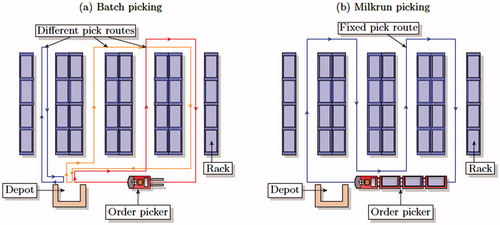
In a milkrun picking system (Figure 1(b)), an order picker picks orders in batches that arrive in real-time and integrates them in the current picking cycle. This subsequently dynamically changes the stops on the order picker’s picking route (Gong and de Koster, 2008). The picker is constantly traveling a fixed route along the aisles of a part or the entire order picking area. Using modern order-picking aids such as pick-by-voice techniques or by a handheld terminal, new pick instructions are received continuously and are included in the current picking cycle. In the case where the lines of an incoming customer order are located either at the current stop or further downstream in the picking route, the picker can pick this order in the current picking cycle. In a traditional batch picking system, an incoming customer order would only be picked in one of the following picking cycles. After the picking cycle has been completed and the order picker reaches the depot, the picked products are disposed and sorted per customer order (i.e., using a pick-and-sort system), and a new picking cycle starts immediately. This way of order picking saves set-up time, worker travel time, and allows fast customer response, particularly for high order arrival rates, which are often experienced in warehouses of e-commerce companies (Gong and de Koster, 2011). In addition, short order throughput times are important, as e-commerce companies are inclined to set their order cut-off times as late as possible while still guaranteeing that orders can be delivered next day or in some cases even the same day.

In this article, we study the mean order throughput time in a milkrun picking system, i.e., the time between a customer order entering the system until the whole order is delivered at the depot. We determine the mean order throughput time of a customer order for three picking strategies: exhaustive, locally-gated, and globally-gated. The order throughput time, strongly depends on the product (or storage) allocation in the order picking area. Typically, an incoming customer order consists of one or more order lines, each for a product stored at a different location within the order picking area. Therefore, in order to achieve short order throughput times products should be allocated in an optimal way in order to increase the probability that an incoming customer order can be included and fully picked in the current picking cycle. For this, we propose an optimization framework for product allocation in a milkrun picking system, in order to minimize the mean order throughput time. This allows us to compare the various strategies with each other for both a large test set and a real-world application. Our results help both designers and managers to create optimal design and control methods to improve the performance of a milkrun picking system.

We model a milkrun picking system accurately using a polling model with simultaneous batch arrivals. Our work extends the work of Gong and de Koster (2008), who also studied a milkrun picking system using a polling model. However, they only considered waiting times of single-line orders, which is the time between the arrival of a customer order and the start of the pick of the single order line within the picking area. This statistic, however, does not capture the required time that is necessary for the order picker to return to the depot, neither does it provide the required time to pick a multi-line order. The current article uses the framework for studying polling systems with simultaneous arrivals of Van der Gaast et al. (2017). Our contribution lies in adapting this framework to a warehousing context, as well as the exact analysis of the mean order throughput times, and the optimization framework for product allocation.

This article is organized as follows: in Section 2, an overview of existing models for milkrun picking systems are presented. In Section 3, a detailed description of the model and the corresponding notation used in this article is given. Section 4 provides the analysis of the mean order throughput time for different picking strategies. In Section 5 and Section 6, the optimization framework is presented, which is used to decide how products should be allocated to the various storage positions in order to minimize the order throughput time of an incoming customer order. We extensively analyze the results of our model and optimization framework in Section 7, via computational experiments for a range of parameters. Finally, in Section 8, we conclude and suggest some extensions of the model and further research topics.

2. Literature review

In internal logistics, e.g., manufacturing or warehousing, a milkrun refers to the cyclic delivery and/or pickup of raw materials, work in process, or finished goods between different locations within the building. The literature on milkrun systems for internal logistics can be categorized into papers that study system performance using simulation methods, and the ones that use analytical models. The most applied method to study a milkrun in a manufacturing setting is simulation, e.g., Hanson and Finnsgård (2014), Korytkowski and Karkoszka (2016) and Staab et al. (2016). These papers generally conclude that a milkrun leads to increased smoothness in the material flows.

Analytical models for milkrun systems for internal logistics are more scarce. Bozer and Ciemnoczolowski (2013) and Ciemnoczolowski and Bozer (2013) analyzed a milkrun system that uses a kanban system to decide which and how many materials should be delivered next to the work centers. Emde and Boysen (2012) and Kilic and Durmusoglu (2013) both studied the joint routing and scheduling in milkrun system in a production setting. Kovcs (2011) developed a deterministic optimization model for product assignment in warehouses served by milkrun logistics. The author proposed a mixed-integer program for product allocation in the milkrun system, and showed that the allocations the model obtained could provide up to 36–38% improvement in order cycle time compared with classic cube-per-order product allocation.

The first paper to study milkrun picking systems where new customer orders can be included in the same picking cycle was presented by Gong and de Koster (2008). The authors refered to the system in their paper as a dynamic order picking system. They used a polling model and showed that the use of a milkrun picking system has a considerable advantage in on-time service completion over traditional batch picking. Boon et al. (2010) considered an efficient enhancement to an ordinary milkrun picking system that allows products to be stored at multiple locations. However, neither of these papers considered multi-line orders and focused only on waiting times of single-line orders. A starting point for this analysis is provided by Van der Gaast et al. (2017) who studied a polling system with simultaneous arrivals. In that paper, a general framework for analyzing the Laplace–Stieltjes transform of the steady-state batch sojourn-time distribution for three service disciplines was developed. Also, a Mean Value Analysis (MVA) approach was developed to calculate performance statistics such as the mean batch sojourn-times, but it also allows, as we will show in this article, to calculate the mean order throughput time.

Kovcs (2011) presented deterministic results that showed that a proper product allocation strategy leads to significantly better system performance. In the literature, four strategies can be identified: randomized storage, dedicated storage, class-based storage, and correlated storage (e.g., Van den Berg (1999)). The last policy is of particular interest for application to the case of multi-line orders, as information is used about which products are ordered together so that they can be stored together in order to reduce travel times for order picking. However, the literature on correlated product allocation is limited, e.g., Frazelle (1990), Kim (1993), Garfinkel (2005), and Xiao and Zheng (2011), and does not address the dynamic aspect of our problem.

3. Model description

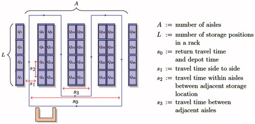
Consider a milkrun picking system as shown in Figure 2. We assume the order picking area to have a parallel aisle layout, with A aisles and L storage positions on each side of an aisle (a rack). Within an aisle, the order picker applies two-sided picking, i.e., simultaneous picking from the right and left sides within an aisle (De Koster et al., 1999). We denote the storage locations by $Q_1,\dots ,Q_N,$ where the number of storage locations N equals 2AL. Each storage location can be considered as a queue for order lines requesting the product stored on that location. We consider that products are stored at one unique pick location, and we assume that the number of storage locations equals the number of different products stored in the warehouse. For ease of presentation, all references to queue indices greater than N or less than one are implicitly assumed to be modulo N, e.g., $Q_{N+1}$ is understood as Q₁. The order picker visits all queues according to a strict S-shape routing strategy in a cyclic sequence and picks all required products for the outstanding customer orders to a pick cart or tow-train. This means that every aisle is completely traversed during a picking cycle, because new customer orders can enter the system in real-time. Therefore, the order picker cannot skip entering an aisle as in conventional batch picking. We assume the number of products the order picker can pick per picking cycle is unconstrained, as for online retailers the route often finishes before the cart or train is full (Gong and de Koster, 2008). This implies that every customer order is either fully picked by the end of the current cycle or at the end of the next cycle. Finite capacity of the pick cart and storing the same product at multiple locations are considered to be further extensions of the model.

Figure 2. Overview of the milkrun picking system.

A milkrun picking system with multi-line customer orders arriving in real-time can be accurately modeled using a polling system with simultaneous batch arrivals (Van der Gaast et al., 2017). Polling systems are multi-queue systems served by a single server who cyclically visits the queues in order to serve the customers waiting at these queues. Typically, when moving from one queue to another the server incurs a switch-over time. In a milkrun picking system, the order picker is represented by the server and a storage location by a queue, and a multi-line order represents multiple simultaneously arriving customers (a batch).

Assume new customer orders arrive at the system according to a Poisson process with rate λ. Each customer order is of size $\mathit{D}=(D_1,\dots ,D_N)$, where D_j, $j=1,\dots ,N$ represents the number of units of product j is requested. Let $\mathit{K}=\Phi (\mathit{D}),$ where $\Phi :{\mathbb{N}}^N\to {\mathbb{N}}^N.$ Mapping $\Phi$ defines the allocation of the products to their storage locations and is given by, $\Phi (\mathit{D})=\mathit{D}x,$ where $x_{ij}\in {\mathbb{N}}^{N\times N}$ with x_ij = 1 if product j is allocated to storage location i and 0 otherwise. Then, for each order, $\mathit{K}=(K_1,\dots K_N),$ where K_i represents the number of units that need to be picked at Q_i, $i=1,\dots ,N$ for that order. The random vector K is assumed to be independent of past and future arriving epochs and for every realization at least one product needs to be picked. The support with all possible realizations of K is denoted by $\mathcal{K}$, and we denote by $\mathit{k}=(k_1,\dots k_N)$ a realization of K. The joint probability distribution of K is denoted by $\pi (k)=\mathbb{P}(K_1=k_1,\dots ,K_N=k_N).$ The arrival rate of product units that need to be picked at Q_i is denoted by $\lambda {}_i=\lambda E(K_i).$ The total arrival rate of product units to be picked for the customer orders arriving in the system is given by $\Lambda ={\sum }_{i=1}^N{\lambda }_i$ The order throughput time of an arbitrary customer order is denoted by T and is defined as the time between its arrival epoch until the order has been fully picked and delivered at the depot.

At each queue, the picker picks the product units on a First-Come First-Served basis. The picking times of a product unit in Q_i is denoted by a generally distributed random variable B_i, with first and second moment $E(B_i)$ and $E(B_i^2),$ which is assumed to be independent and identically distributed. The workload at Q_i, $i=1,\dots ,N$ is defined by ${\rho }_i={\lambda }_{i}E(B_i);$ the overall system load by $\rho ={\sum }_{i=1}^N{\rho }_i$. For the system to be stable a necessary and sufficient condition is that $\rho \hspace{0.17em}<\hspace{0.17em}1$ (Takagi, 1986), which is assumed to be the case in the remainder of this article.

When the order picker moves from Q_i to $Q_{i+1},$ he or she takes a generally distributed travel time S_i with first and second moment $E(S_i)$ and $E(S_i^2).$ Without loss of generality, we assume that the travel times from side to side within an aisle are independent and identically distributed with mean s₁ and second moment $s_1^2,$ the travel times within aisles between two adjacent storage locations have mean s₂ and second moment $s_2^2,$ whereas the time required to travel from one aisle to the next one has mean s₃ and second moment $s_3^2.$ Finally, after visiting the last queue the order picker returns to the first queue to start a new cycle. On the way, the order picker visits the depot where he or she will drop off the picked products so that other operators can sort and transport them. We assume that this time is independent of the number of products picked, and it is included in s₀ and its second moment $s_0^2.$ See also Figure 2. Let $E(S)={\sum }_{i=1}^{N}E(S_i)=s_0+A\cdot L\cdot s_1+A\cdot (L-1)\cdot s_2+(A-1)\cdot s_3$ be the total expected travel time in a cycle and $E(S^2)={\sum }_{i=1}^{N}E(S_i^2)+\sum _{i\ne j}E(S_i)E(S_j)$ its second moment. Note that storing different products vertically can easily be incorporated in the model by increasing the number of storage locations and defining a new switch-over time between storage locations within the same shelf.

We define a picking cycle from the service beginning at the first queue until the order picker has delivered all the picked products at the depot and arrives at the first queue again. Therefore, a picking cycle C consists of N visit periods, V_i, each followed by a travel time S_i. A visit period V_i starts with a pick of a product unit and ends after the last product has been picked, given that product units need to be picked at Q_i. Then, the order picker travels to the next picking location of which the duration is S_i. In the case where no product units need to be picked at Q_i the order picker immediately travels to next picking location. The total mean duration of a picking cycle is independent of the queues involved (and the picking strategies that are considered) and is given by (see, e.g., Takagi (1986))$E(C)=E(S)/(1-\rho ).$ Finally, we assume replenishment is not required in a picking cycle, and each queue has infinite capacity (i.e., no limit on the maximum number of order lines waiting to be picked).

The picking strategy at each queue follows one of the service disciplines that have been extensively considered in previous research on polling systems (see, e.g., Boon et al. (2011) for an overview of polling literature). Under the exhaustive strategy, the order picker picks all product units at the current queue until no product units need to be picked anymore. This also includes demand for the product that arrives while the picker is busy picking at this queue. On the other hand, under the locally-gated strategy, the order picker only picks the product units that need to be picked at the start of the first pick at a queue; all demand that arrives during the course of the visit will be picked in the next visit. Finally, for the globally-gated strategy the picker will not pick any products of incoming customer orders that arrived during the current picking cycle. Only after the start of the next picking cycle will these incoming orders be picked. Note that this strategy is similar to conventional batch picking with high order arrival rates and flexible batch sizes, given that the order picker has to visit all the picking locations during a picking tour, delivers all the picked products at the depot and immediately continues with the next tour. Similar to in batch picking, no orders can be included during the current picking cycle.

Whether a customer order is fully picked in the picking cycle during which it arrives, or otherwise in the next cycle depends on the location of the picker and the picking strategy. Therefore, let ${\mathcal{K}}_j^0$ and ${\mathcal{K}}_j^0,j=1,\dots ,N$ be subsets of support $\mathcal{K}$, defined as $${\mathcal{K}}_j^0=\left\{k_1=0,\dots ,k_{j-1}=0,k_j\ge 0,k_{j+1}\ge 0,\dots ,k_N\ge 0\right\}\in \mathcal{K},$$ and ${\mathcal{K}}_j^1={({\mathcal{K}}_j^0)}^c$ as its complement such that for $j=1,\dots ,N$ we have ${\mathcal{K}}_j^0\cup {\mathcal{K}}_j^1=\mathcal{K}$ and let the associated probabilities be $\pi ({\mathcal{K}}_j^0)$ and $\pi ({\mathcal{K}}_j^1).$ The interpretation of $\mathit{k}\in K_j^0$ is that for an incoming customer order all the products need to be picked at $Q_j,\dots ,Q_N.$ For example, in the case of the exhaustive strategy, this means that if the order picker is at Q_j or has not reached Q_j yet a customer order $\mathit{k}\in {\mathcal{K}}_j^0$ can be included in the current picking cycle, whereas if $k\in {\mathcal{K}}_j^1$ the order will be completed in the next cycle. Finally, let $E(K_i|{\mathcal{K}}_j^0)$ and $E(K_i|{\mathcal{K}}_j^1)$ be the conditional mean number of product units that need to picked in Q_i, $i=1,\dots ,N$ given subset ${\mathcal{K}}_j^0$ or ${\mathcal{K}}_j^1$.

In the next section the mean order throughput time is derived for the three picking strategies.

4. Mean order throughput time

4.1. Exhaustive strategy

In order to derive the mean order throughput time for the exhaustive strategy, we apply the MVA approach of Van der Gaast et al. (2017). In this MVA approach, a set of N² linear equations is derived for calculating $E({\overline{L}}_i^{(S_{j-1,}{V}_j)}),$ the conditional mean queue-length at Q_i (excluding the potential product unit that is being picked) at an arbitrary epoch within travel period $S_{j-1}$ and visit period V_j. These MVA equations are given in online supplement A and are based on standard queueing results, i.e., the Poisson arrivals see time averages (PASTA) property (Wolff, 1982) and Little’s Law (Little, 1961). With use of the conditional mean queue-lengths, not only can the performance statistics such as the waiting time of a customer be determined, but also the mean order throughput time as we will show in this section.

For notation purposes we introduce θ_j in this section as shorthand for intervisit period $(S_{j-1},V_j);$ the mean duration of this period $E({\theta }_j)$ is given by, $E({\theta }_j)=E(S_{j-1})+E(V_j),$$j=1,\dots ,N,$ where $E(V_j)={\rho }_{j}E(C)$ corresponds with the mean time to pick all incoming products during a cycle at location j and ${\sum }_{j=1}^{N}E({\theta }_j)=E(C).$

In addition, we use $d_{j,n}$ to denote the total mean work in $Q_{j+1},\dots ,Q_{j+n},$ which originates from customer orders that arrive per unit of pick time B_j or travel time $S_{j-1},$ and all the subsequent picks that are triggered by these picks before the picker finishes service in $Q_{j+n}$. For example, a single product pick in Q_j will generate on average additional work in $Q_{j+1},\dots ,Q_{j+n}$ of duration $E(B_j)d_{j,n}.$ Then $d_{j,0}=0$ and for n > 0 we have: (1) $$d_{j,n}=\sum _{m=1}^n{\delta }_{j,m},j=1,\dots ,N,$$(1) where ${\delta }_{j,m}$ is the contribution of $Q_{j+m}.$ First, ${\delta }_{j,1}={\rho }_{j+1}/(1-{\rho }_{j+1})$ includes the mean picking times and the consecutive busy periods in $Q_{j+1}$ of product units that arrived during a product pick B_j or travel time $S_{j-1}$. Then, ${\delta }_{j,2}=(1+{\delta }_{j,1}){\rho }_{j+2}/(1-{\rho }_{j+2})$ contains the mean picking times of the product units that arrived in $Q_{j+2}$ during B_j or $S_{j-1}$ and the previous busy periods in $Q_{j+1}$ plus all the busy periods that these picks generate in $Q_{j+2}$. 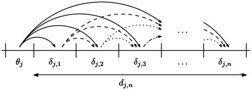In general we can write ${\delta }_{j,n}$ for n > 0 as (see Figure 3): $${\delta }_{j,n}=\sum _{m=1}^{\min \left(N-1,n\right)}{\delta }_{j,n-m}\frac{{\rho }_{j+n}}{1-{\rho }_{j+n}},j=1,\dots ,N,$$ where ${\delta }_{j,0}=1.$ For example, if j = 4, n = 5, and N = 6, then $${\delta }_{4,5}={\sum }_{m=1}^{\min (6-1,5)}{\delta }_{4,5-m}\frac{{\rho }_{4+5}}{1-{\rho }_{4+5}}=\left[{\delta }_{4,4}+{\delta }_{4,3}+{\delta }_{4,2}+{\delta }_{4,1}+{\delta }_{4,0}\right]\frac{{\rho }_3}{1-{\rho }_3}.$$ Note that ${\delta }_{j,n}$ only depends on at most N − 1 previous ${\delta }_{j,n-m}$, as since if new demand arrives at the queue that is currently being visited it will be picked before the end of the current visit.

Figure 3. Description of d_j,n.

The mean order throughput time $E(T^{EX})$ for the exhaustive strategy can be determined by explicitly conditioning on the location of the order picker and by studying the system until the incoming customer order has been fully delivered at the depot: (2) $$E\left(T^{EX}\right)=\frac{1}{E\left(C\right)}\sum _{j=1}^{N}E\left({\theta }_j\right)(\pi \left({\mathcal{K}}_j^0\right)E\left(T^{\left({\theta }_j,0\right)}\right)+\pi \left({\mathcal{K}}_j^1\right)E\left(T^{\left({\theta }_j,1\right)}\right)).$$(2)

Whenever the order picker is at intervisit period θ_j and still can pick all the products of an incoming customer order (i.e., $\mathit{k}\in {\mathcal{K}}_j^0$), then the order throughput time is equal to $E(T^{({\theta }_j,0)})$. This is the mean time until the order picker reaches the depot during the current cycle including the conditional mean number of picks for customer orders in $\mathit{k}\in {\mathcal{K}}_j^0$. Otherwise, one or more products are located upstream and the order throughput time is equal to $E(T^{({\theta }_j,0)})$. This is the expected time until the order picker reaches the depot in the next cycle including the conditional mean number of picks for customer orders in $\mathit{k}\in {\mathcal{K}}_j^1.$

First, we focus on the derivation of $E(T^{({\theta }_j,0)})$. When the customer order enters the system in intervisit period θ_j with probabilities $E(V_j)/E({\theta }_j)$ and $E(S_{j-1})/E({\theta }_j)$ it has to wait for a residual picking time $E(B_j^R)=E(B_j^2)/(2E(B_j))$ or residual travel time $E(S_{j-1}^R)=E(S_{j-1}^2)/(2E(S_{j-1})).$ Also, it has to wait for $E(L_j^{-({\theta }_j)})$ product units that still need to be picked at Q_j, as well as the expected $E({\mathcal{K}}_j|{\mathcal{K}}_j^0)$ product units that need be picked at this queue for a customer order in $\mathit{k}\in K_j^0.$ Each of these picks triggers a busy period of length $E(B_j)/(1-{\rho }_j)$ and generates additional picks that will be made before the end of the current cycle of duration $d_{j,N-j}E(B_j)/(1-{\rho }_j).$ This also applies for the residual picking time and residual travel time. Then, for each subsequent intervisit period θ_l, $l=j+1,\dots ,N$, the travel time from $Q_{l-1}$ to Q_l will trigger a busy period and additional picks in $Q_l,\dots ,Q_N$ of duration $E(S_{l-1})(1+d_{l,N-l})/(1-{\rho }_l).$ Similarly, the average number of product units that still needed to be picked at the customer order arrival and the mean $E(K_l|{\mathcal{K}}_j^0)$ product units needed to be picked for the arriving customer order will increase the mean order throughput time by $\left[E(L_l^{-({\theta }_j)})+E(K_l|{\mathcal{K}}_j^0)\right]E(B_l)(1+d_{l,N-l})/(1-{\rho }_l).$ Finally, the picked orders have to be delivered to the depot of which the duration is $E(S_N).$

Combining this gives the following expression for the mean time until the order picker reaches the depot during the current cycle given the average number of picks for a customer order in $\mathit{k}\in {\mathcal{K}}_j^0:$ (3) $$E\left(T^{\left({\theta }_j,0\right)}\right)=(\frac{E\left(V_j\right)}{E\left({\theta }_l\right)}E\left(B_j^R\right)+\frac{E\left(S_{j-1}\right)}{E\left({\theta }_j\right)}E\left(S_{j-1}^R\right)+\left[E\left(L_j^{-\left({\theta }_j\right)}\right)+E\left(K_j|{\mathcal{K}}_j^0\right)E\left(B_j\right)\right])\times \frac{1+d_{j,N-j}}{1-{\rho }_j}+\sum _{l=1}^{N-j}(E\left(S_{j+l-1}\right)+\left[E\left(L_{j+l}^{-\left({\theta }_j\right)}\right)+E\left(K_{j+l}|{\mathcal{K}}_j^0\right)\right]E\left(B_{j+1}\right))\times \frac{1+d_{j+1,N-j-l}}{1-{\rho }_{j+l}}+E\left(S_N\right).$$(3)

Next we focus on $E(T^{({\theta }_j,1)}).$ The derivation is similar to the one of Equation (3)(3) $$E\left(T^{\left({\theta }_j,0\right)}\right)=(\frac{E\left(V_j\right)}{E\left({\theta }_l\right)}E\left(B_j^R\right)+\frac{E\left(S_{j-1}\right)}{E\left({\theta }_j\right)}E\left(S_{j-1}^R\right)+\left[E\left(L_j^{-\left({\theta }_j\right)}\right)+E\left(K_j|{\mathcal{K}}_j^0\right)E\left(B_j\right)\right])\times \frac{1+d_{j,N-j}}{1-{\rho }_j}+\sum _{l=1}^{N-j}(E\left(S_{j+l-1}\right)+\left[E\left(L_{j+l}^{-\left({\theta }_j\right)}\right)+E\left(K_{j+l}|{\mathcal{K}}_j^0\right)\right]E\left(B_{j+1}\right))\times \frac{1+d_{j+1,N-j-l}}{1-{\rho }_{j+l}}+E\left(S_N\right).$$(3) , except that we should also consider the additional demand that is generated during a pick or a switch from queue to queue until the end of the next picking cycle. This gives the following expression: (4) $$E\left(T^{\left({\theta }_j,1\right)}\right)=(\frac{E\left(V_j\right)}{E\left({\theta }_j\right)}E\left(B_j^R\right)+\frac{E\left(S_{j-1}\right)}{E\left({\theta }_j\right)}E\left(S_{j-1}^R\right)+\left[E\left(L_j^{-\left({\theta }_j\right)}\right)+E\left(K_j|{\mathcal{K}}_j^1\right)\right]E\left(B_j\right))\times \frac{1+d_{j,2N-j}}{1-{\rho }_j}+\sum _{l=1}^{N-1}(E\left(S_{j+l-1}\right)+\left[E\left(L_{j+l}^{-\left({\theta }_j\right)}\right)+E\left(K_{j+l}|{\mathcal{K}}_j^1\right)\right]E\left(B_{j+1}\right))\times \frac{1+d_{j+l,2N-j}}{1-{\rho }_j}+\sum _{l=N}^{2N-j}E\left(S_{j+l-1}\right)\frac{1+d_{j+l,2N-j-l}}{1-{\rho }_{j+l}}+E\left(S_N\right).$$(4)

Then, $E(T^{EX})$in Equation (2)(2) $$E\left(T^{EX}\right)=\frac{1}{E\left(C\right)}\sum _{j=1}^{N}E\left({\theta }_j\right)(\pi \left({\mathcal{K}}_j^0\right)E\left(T^{\left({\theta }_j,0\right)}\right)+\pi \left({\mathcal{K}}_j^1\right)E\left(T^{\left({\theta }_j,1\right)}\right)).$$(2) can be easily calculated with use of Equations (3)(3) $$E\left(T^{\left({\theta }_j,0\right)}\right)=(\frac{E\left(V_j\right)}{E\left({\theta }_l\right)}E\left(B_j^R\right)+\frac{E\left(S_{j-1}\right)}{E\left({\theta }_j\right)}E\left(S_{j-1}^R\right)+\left[E\left(L_j^{-\left({\theta }_j\right)}\right)+E\left(K_j|{\mathcal{K}}_j^0\right)E\left(B_j\right)\right])\times \frac{1+d_{j,N-j}}{1-{\rho }_j}+\sum _{l=1}^{N-j}(E\left(S_{j+l-1}\right)+\left[E\left(L_{j+l}^{-\left({\theta }_j\right)}\right)+E\left(K_{j+l}|{\mathcal{K}}_j^0\right)\right]E\left(B_{j+1}\right))\times \frac{1+d_{j+1,N-j-l}}{1-{\rho }_{j+l}}+E\left(S_N\right).$$(3) and (4)(4) $$E\left(T^{\left({\theta }_j,1\right)}\right)=(\frac{E\left(V_j\right)}{E\left({\theta }_j\right)}E\left(B_j^R\right)+\frac{E\left(S_{j-1}\right)}{E\left({\theta }_j\right)}E\left(S_{j-1}^R\right)+\left[E\left(L_j^{-\left({\theta }_j\right)}\right)+E\left(K_j|{\mathcal{K}}_j^1\right)\right]E\left(B_j\right))\times \frac{1+d_{j,2N-j}}{1-{\rho }_j}+\sum _{l=1}^{N-1}(E\left(S_{j+l-1}\right)+\left[E\left(L_{j+l}^{-\left({\theta }_j\right)}\right)+E\left(K_{j+l}|{\mathcal{K}}_j^1\right)\right]E\left(B_{j+1}\right))\times \frac{1+d_{j+l,2N-j}}{1-{\rho }_j}+\sum _{l=N}^{2N-j}E\left(S_{j+l-1}\right)\frac{1+d_{j+l,2N-j-l}}{1-{\rho }_{j+l}}+E\left(S_N\right).$$(4) .

4.2. Locally-gated strategy

The mean order throughput time in the case of the locally-gated strategy can be calculated in a similar way as the exhaustive strategy. For the locally-gated strategy, per queue all incoming demand is placed before a gate. Only at the start of a visit period at a queue, all product units that need be picked at this location are placed behind the gate, which means that the order picker will pick these product units in the current picking cycle. For this we slightly redefine ${\mathcal{K}}_j^0=\left\{k_1=0,\dots ,k_{j-1}=k_j=0,k_{j+1}\ge 0,\dots ,k_N\ge 0\right\}\in \mathcal{K}$ to reflect this change.

First, we introduce θ_j in this section as shorthand for intervisit period$(V_j,S_j);$ the expected duration of this period $E({\theta }_j)$ is given by, $E({\theta }_j)=E(V_j)+E(S_j),$$j=1,\dots ,N.$ In contrast with the exhaustive strategy, we have to make a distinction between the mean number of product units before and behind the gate. We introduce variables $E({\tilde{L}}_i^{({\theta }_j)}),i,j=1,\dots ,N$ as the conditional mean queue-length of product units located before the gate in Q_i during intervisit period θ_j and $E({\widehat{L}}_i^{({\theta }_i)}),i=1,\dots ,N$ as the conditional mean queue-length of product units located behind the gate in Q_i during intervisit period θ_i. In the MVA approach proposed by Van der Gaast et al. (2017) a set of $N(N+1)$ linear equations is derived for calculating these conditional mean queue-lengths, which we will use in order to determine the order throughput time. These equations are given in online supplement B.

Similar to the exhaustive strategy, we introduce $d_{j,n}$ which is defined as Equation (1)(1) $$d_{j,n}=\sum _{m=1}^n{\delta }_{j,m},j=1,\dots ,N,$$(1) , but ${\delta }_{j,n}$ changes because of the different picking strategy. First, ${\delta }_{j,1}={\rho }_{j+1}$ contains the mean picking times of all product units in $Q_{j+1}$ that arrive per unit of a product pick B_j or a travel time S_j, whereas ${\delta }_{j,2}={\rho }_{j+2}(1+{\delta }_{j,1})$ also includes the mean picking times of the product units that arrived in $Q_{j+2}$ during a product pick B_j or a travel time S_j, as well as in ${\delta }_{j,1}.$ In general we can write ${\delta }_{j,n}$ for n > 0 as $${\delta }_{j,n}=\sum _{m=1}^{\min \left(N,n\right)}{\delta }_{j,n-m}{\rho }_{j+n},\hspace{1em}j=1,\dots ,.N.$$ where ${\delta }_{j,0}=1.$ In this case ${\delta }_{j,n}$ depends on N previous ${\delta }_{j,n-m}$ because if new demand arrives at the queue that is currently being visited it will not be picked during the current cycle.

Similar to Equation (2)(2) $$E\left(T^{EX}\right)=\frac{1}{E\left(C\right)}\sum _{j=1}^{N}E\left({\theta }_j\right)(\pi \left({\mathcal{K}}_j^0\right)E\left(T^{\left({\theta }_j,0\right)}\right)+\pi \left({\mathcal{K}}_j^1\right)E\left(T^{\left({\theta }_j,1\right)}\right)).$$(2) , we condition on the location of the order picker and determine if the customer order can be picked during the current picking cycle, or the next. Then (5) $$E\left(T^{LG}\right)=\frac{1}{E\left(C\right)}\sum _{j=1}^{N}E\left({\theta }_j\right)(\pi \left({\mathcal{K}}_j^0\right)E\left(T^{\left({\theta }_j,0\right)}\right)+\pi \left({\mathcal{K}}_j^1\right)E\left(T^{\left({\theta }_j,1\right)}\right)).$$(5)

First, we consider $E(T^{({\theta }_j,0)})$ in the case where a customer order $\mathit{k}\in {\mathcal{K}}_j^0$ arrives during intervisit period θ_j and will be fully picked and delivered to the depot at the end of the current cycle. With probability $E(V_j)/E({\theta }_j)$ the arriving customer order has to wait for the order picker to finish the current pick and the travel time to the next queue, whereas with probability $E(S_j)/E({\theta }_j)$ the order only has wait for the residual travel time. Also, there are $E({\widehat{L}}_i^{({\theta }_i)})$ product units behind the gate that need still to be picked, for which each pick has duration $E(B_j).$ During the residual time in θ_j new demand is generated at $Q_{j+1},\dots ,Q_N$ that will be picked before the end of the current picking cycle. Then, for Q_l, $l=j+1,\dots N,E({\tilde{L}}_l^{({\theta }_j)})$product units need to be picked for customer orders that were already in the system, as well as $E(K_l|{\mathcal{K}}_j^0)$, the average number of product units to be picked for the arriving order. Each of these picks has duration $E(B_l)$, during which new customer orders might arrive which generate additional picks at the queues that still need to be visited during the current cycle. Similar during all the remaining travel times, new customer orders can arrive that will generate additional picks at the queues that still need to be visited before the order picker reaches the depot. This gives the following expression: (6) $$E\left(T^{\left({\theta }_j,0\right)}\right)=(\frac{E\left(V_j\right)}{E\left({\theta }_j\right)}\left(E\left(B_j^R\right)+E\left(S_j\right)\right)+\frac{E\left(S_j\right)}{E\left({\theta }_j\right)}E\left(S_j^R\right)+E\left({\widehat{L}}_j^{\left({\theta }_j\right)}\right)E\left(B_j\right))\times \left(1+d_{j,N-j}\right)\times \sum _{l=1}^{N-j}\left(\left[E\left({\tilde{L}}_{j+1}^{\left({\theta }_j\right)}\right)+E\left(K_{j+1}|{\mathcal{K}}_j^0\right)\right]E\left(B_{j+l}\right)+E\left(S_{j+l}\right)\right)\times \left(1+d_{j+l,N-j-l}\right).$$(6)

The derivation of $E(T^{({\theta }_j,1)})$ is similar, except that customer orders will be delivered at the depot the next picking cycle. Therefore, we should also consider the additional demand that is generated during a pick or a switch from queue to queue until the end of the next picking cycle. This gives the following expression: (7) $$E\left(T^{\left({\theta }_j,1\right)}\right)=(\frac{E\left(V_j\right)}{E\left({\theta }_j\right)}\left(E\left(B_j^R\right)+E\left(S_j\right)\right)+\frac{E\left(S_j\right)}{E\left({\theta }_j\right)}E\left(S_j^R\right)+E\left({\widehat{L}}_i^{\left({\theta }_i\right)}\right)E\left(B_i\right))\times \left(1+d_{j,2N-j}\right)+\sum _{l=1}^N(\left[E\left({\tilde{L}}_{j+1}^{\left({\theta }_j\right)}\right)+E\left(K_{j+l}|{\mathcal{K}}_j^1\right)\right]E\left(B_{j+l}\right)+E\left(S_{j+l}\right))\times \left(1+d_{j+l,2N-j-l}\right)+\sum _{l=N+1}^{2N-j}E\left(S_{j+l}\right)\left(1+d_{j+l,2N-j-l}\right).$$(7)

Then, $E(T^{LG})$in Equation (5)(5) $$E\left(T^{LG}\right)=\frac{1}{E\left(C\right)}\sum _{j=1}^{N}E\left({\theta }_j\right)(\pi \left({\mathcal{K}}_j^0\right)E\left(T^{\left({\theta }_j,0\right)}\right)+\pi \left({\mathcal{K}}_j^1\right)E\left(T^{\left({\theta }_j,1\right)}\right)).$$(5) can be easily calculated with the use of Equations (6)(6) $$E\left(T^{\left({\theta }_j,0\right)}\right)=(\frac{E\left(V_j\right)}{E\left({\theta }_j\right)}\left(E\left(B_j^R\right)+E\left(S_j\right)\right)+\frac{E\left(S_j\right)}{E\left({\theta }_j\right)}E\left(S_j^R\right)+E\left({\widehat{L}}_j^{\left({\theta }_j\right)}\right)E\left(B_j\right))\times \left(1+d_{j,N-j}\right)\times \sum _{l=1}^{N-j}\left(\left[E\left({\tilde{L}}_{j+1}^{\left({\theta }_j\right)}\right)+E\left(K_{j+1}|{\mathcal{K}}_j^0\right)\right]E\left(B_{j+l}\right)+E\left(S_{j+l}\right)\right)\times \left(1+d_{j+l,N-j-l}\right).$$(6) and (7)(7) $$E\left(T^{\left({\theta }_j,1\right)}\right)=(\frac{E\left(V_j\right)}{E\left({\theta }_j\right)}\left(E\left(B_j^R\right)+E\left(S_j\right)\right)+\frac{E\left(S_j\right)}{E\left({\theta }_j\right)}E\left(S_j^R\right)+E\left({\widehat{L}}_i^{\left({\theta }_i\right)}\right)E\left(B_i\right))\times \left(1+d_{j,2N-j}\right)+\sum _{l=1}^N(\left[E\left({\tilde{L}}_{j+1}^{\left({\theta }_j\right)}\right)+E\left(K_{j+l}|{\mathcal{K}}_j^1\right)\right]E\left(B_{j+l}\right)+E\left(S_{j+l}\right))\times \left(1+d_{j+l,2N-j-l}\right)+\sum _{l=N+1}^{2N-j}E\left(S_{j+l}\right)\left(1+d_{j+l,2N-j-l}\right).$$(7) .

4.3. Globally-gated strategy

The final strategy for which we derive the mean order throughput time is the globally-gated strategy. This strategy resembles the locally-gated strategy, except that we only pick the product units that need to be picked during the start of a picking cycle, instead of the start of a visit period to a queue. This implies that every incoming customer order will only be picked during the next picking cycle. As a result, the analysis of this strategy is more straightforward compared with the other two strategies.

The mean order throughput time can be determined as follows. First, any incoming order first has to wait for the current residual cycle time. Then, the duration of the next picking cycle equals all the picks for incoming orders that have already arrived at the system before the incoming order in the same cycle and those that arrived during the residual cycle time. In addition, the average duration of all the picks for a customer order and the total travel time in one cycle increase the mean order throughput time. This gives the following expression: (8) $$E\left(T^{GG}\right)=E\left(C_R\right)+\sum _{j=1}^N{\lambda }_{j}E\left(B_j\right)\left(E\left(C_p\right)+E\left(C_R\right)\right)+\sum _{j=1}^{N}E\left(S_j\right)+\sum _{j=1}^{N}E\left(K_j\right)E\left(B_j\right)=\left(1+2\rho \right)\frac{E\left(C^2\right)}{2E\left(C\right)}+E\left(S\right)+\sum _{j=1}^{N}E\left(K_j\right)E\left(B_j\right),$$(8) where $E(C_p)$ and $E(C_R)$ are the mean past and residual cycle time. From Van der Gaast et al. (2017) we know that $E(C_p)=E(C_R)=E(C^2)/(2E(C)),$ and $$\begin{array}{l}E\left(C^2\right)=\frac{1}{\left(1-{\rho }^2\right)}[E\left(S^2\right)+2\rho E\left(S\right)E\left(C\right)+\sum _{j=1}^N{\lambda }_{j}E\left(B_j^2\right)E\left(C\right)\\ +\sum _{i=1}^N\lambda \left(E\left(K_i^2\right)-E\left(K_i\right)\right)E{\left(B_i\right)}^{2}E\left(C\right)+\sum _{i,j:i\ne j}^N\lambda E\left(K_i{K}_j\right)E\left(B_i\right)E\left(B_j\right)E\left(C\right)].\end{array}$$

5. Optimization model for product allocation

The performance of the milkrun picking system largely depends on the product allocation. A good product allocation allows many customer orders to be picked in the current picking cycle and delivered to the depot as soon as possible. Therefore, we formulate an optimization model to find a product allocation x that minimizes the mean order throughput time. For each of the three picking strategies we minimize the mean order throughput time $E(T^d(x)),$ where $d\in \left\{EX,LG,GG\right\}$ denotes the picking strategy and x defines the product allocation. As explained in Section 3, the mean order throughput time depends on allocation x, due to the allocation determining how many units on average need to be picked per storage location, $E(K_i),i=1,\dots ,N,$ which in turn determines the arrival rate and utilization per storage location, λ_i and ρ_i, respectively.

We define the following integer programming model; (9) $$\text{minimize}\hspace{0.5em}E\left(T^d\left(x\right)\right),$$(9) (10) $$\text{subject} \text{to}\sum _{j=1}^N{x}_{ij}=1\hspace{0.5em}\text{for}\hspace{0.5em}\text{all}\hspace{0.5em}i\in N,$$(10) (11) $$\sum _{i=1}^N{x}_{ij}=1\hspace{0.5em}\text{for}\hspace{0.5em}\text{all}\hspace{0.5em}j\in N,$$(11) (12) $$x_{ij}\in \left\{0,1\right\}\hspace{0.5em}\text{for}\hspace{0.5em}\text{all}\hspace{0.5em}i,j\in N.$$(12)

The objective of model (9) is to minimize the mean order throughput time (Equations (2)(2) $$E\left(T^{EX}\right)=\frac{1}{E\left(C\right)}\sum _{j=1}^{N}E\left({\theta }_j\right)(\pi \left({\mathcal{K}}_j^0\right)E\left(T^{\left({\theta }_j,0\right)}\right)+\pi \left({\mathcal{K}}_j^1\right)E\left(T^{\left({\theta }_j,1\right)}\right)).$$(2) , (5)(5) $$E\left(T^{LG}\right)=\frac{1}{E\left(C\right)}\sum _{j=1}^{N}E\left({\theta }_j\right)(\pi \left({\mathcal{K}}_j^0\right)E\left(T^{\left({\theta }_j,0\right)}\right)+\pi \left({\mathcal{K}}_j^1\right)E\left(T^{\left({\theta }_j,1\right)}\right)).$$(5) , or (8) evaluated for product allocation x) given picking strategy d. Constraints (10) ensure that each storage location has only one type of product assigned to it. On the other hand, constraints (11) define that each type of product should be stored at only one storage location. Finally, constraints (12) are the integrality constraints.

From Equations (2)(2) $$E\left(T^{EX}\right)=\frac{1}{E\left(C\right)}\sum _{j=1}^{N}E\left({\theta }_j\right)(\pi \left({\mathcal{K}}_j^0\right)E\left(T^{\left({\theta }_j,0\right)}\right)+\pi \left({\mathcal{K}}_j^1\right)E\left(T^{\left({\theta }_j,1\right)}\right)).$$(2) , (5)(5) $$E\left(T^{LG}\right)=\frac{1}{E\left(C\right)}\sum _{j=1}^{N}E\left({\theta }_j\right)(\pi \left({\mathcal{K}}_j^0\right)E\left(T^{\left({\theta }_j,0\right)}\right)+\pi \left({\mathcal{K}}_j^1\right)E\left(T^{\left({\theta }_j,1\right)}\right)).$$(5) , and (8)(8) $$E\left(T^{GG}\right)=E\left(C_R\right)+\sum _{j=1}^N{\lambda }_{j}E\left(B_j\right)\left(E\left(C_p\right)+E\left(C_R\right)\right)+\sum _{j=1}^{N}E\left(S_j\right)+\sum _{j=1}^{N}E\left(K_j\right)E\left(B_j\right)=\left(1+2\rho \right)\frac{E\left(C^2\right)}{2E\left(C\right)}+E\left(S\right)+\sum _{j=1}^{N}E\left(K_j\right)E\left(B_j\right),$$(8) it can be seen that objective function (9) is nonlinear. Therefore, we cannot apply standard integer programming techniques to find the product allocation that minimizes the mean order throughput time. In the next section we introduce a meta-heuristic that overcomes this issue.

6. A meta-heuristic for product allocation

In order to solve the nonlinear optimization problem of Section 5 we apply a Genetic Algorithm to obtain a product allocation that minimizes the mean order throughput time. Genetic Algorithms (GAs) have been used to successfully solve nonlinear optimization problems for which exact or exhaustive methods are not feasible due to the prohibitive complexity of the problem; they have already been applied in many different fields (see, e.g., Tsai et al. (2008) and Bottani et al. (2012) in the context of order picking).

The first step of the GA is to describe the population of chromosomes and to calculate the fitness of each chromosome. We denote H^g as the gth generation population, where: (13) $$H^g=\left\{y_1^g,y_2^g,\dots ,y_l^g,\dots ,y_M^g\right\},$$(13) consists of a total of M different chromosomes each representing a product allocation. A chromosome is represented by $y_l^g=\left\{y_{l,1}^g,y_{l,2}^g,\dots ,y_{l,j}^g,\dots ,y_{l,N}^g\right\},$ where gene $y_{l,j}^g$ denotes the allocated storage location for product j. In order to calculate the fitness of chromosome $y_l^g$, we determine its associated product allocation $x_l^g$ such that we can evaluate $E(T^d(x_l^g))$ for a given picking strategy d. For this we define $x_l^g=\psi (y_l^g),$ where $\psi :{\mathbb{N}}^N\to {\left\{0,1\right\}}^{N\times N}.$ The mapping ψ is given by, $\psi (y_l^g)=\left[e_{y_l^g,1},e_{y_l^g,2},\dots ,e_{y_l^g,N}\right],$ where e_j denotes a column vector of length N with 1 in the jth position and 0 in every other position. The fitness of population H^g, $F(H^g)$, can now be calculated by (14) $$\begin{array}{l}F\left(H^g\right)=\left\{F\left(y_1^g\right),F\left(y_2^g\right),\dots ,F\left(y_M^g\right)\right\}\\ =\left\{E\left(T^d\left(\psi \left(y_1^g\right)\right)\right),E\left(T^d\left(\psi \left(y_2^g\right)\right)\right),\dots ,E\left(T^d\left(\psi \left(y_M^g\right)\right)\right)\right\}.\end{array}$$(14)

In order to construct the next generation of chromosomes, we select a survivor and an offspring population using the current generation that together form the next generation. First, survivors are chromosomes that are selected from the current population and are then placed in the next generation. Second, offspring are created by mutating and/or recombining current chromosomes in order to create new product allocations. For the offspring population, we select chromosomes based on roulette-wheel selection, also known as stochastic sampling with replacement (Mitchell, 1998). This method determines, for each chromosome, a probability proportional to its fitness as follows: (15) $$p_l=\frac{F\left(y_l^g\right)}{{\sum }_{j=1}^{M}F\left(y_j^g\right)},l=1,\dots ,M.$$(15)

Then, chromosomes with a higher probability have a higher chance of being selected to be used to generate offspring. For the survivor population, we use tournament selection. In this method t_size chromosomes are randomly selected and then the chromosome with best fitness is chosen to generate the survivor population. Finally, the size of the survivor and offspring population is controlled by parameter $0\le \alpha \le 1.$ In every generation $\lfloor \alpha M\rfloor$ chromosomes are selected used to generate offspring, whereas $M-\lfloor \alpha M\rfloor$ selected chromosomes will become the survivor population.

The offspring is generated using a combination of two types of genetic operators: recombination and mutation. First, recombination generates new chromosomes by combining different parts of more than one parent's chromosomes. Second, mutation is carried out by altering one or more genes from their original state of a single chromosome in order to form a new allocation. The operators in the GA were carefully chosen after running initial tests to allow for sufficient recombination and mutation in every generation.

The first operator used in the GA is the Swap Mutation (SM). The SM operator chooses one random gene in a single chromosome and swaps it with one of the remaining genes of the chromosome.

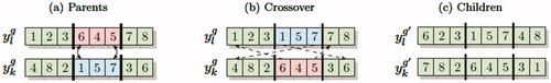
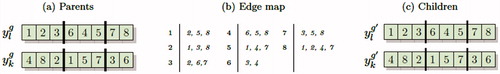
The second operator used is partially matched crossover (PMX). PMX is the recombination operator that uses a subset of genes between two randomly chosen cut points from one parent and completes the remaining part of the child chromosome by preserving the order and positions of as many storage locations as possible from the other parent (Goldberg and Lingle, 1985). For example, in Figure 4 we assume two parent chromosomes $y_l^g$ and $y_k^g$ each consisting of eight genes and two cut points. By crossing-over the subset of genes between the two cut points, two children $y_l^{g^{\prime }}$ and $y_k^{g^{\prime }}$ can be constructed with the following mapping:, $6\leftrightarrow 1,4\leftrightarrow 5,5\leftrightarrow 7.$ Using mapping, the duplicate genes are interchanged until both child chromosomes provide a feasible product allocation.

Figure 4. Example of the partially matched crossover operator.

The third operator is the edge recombination crossover (ERX). The idea of the ERX operator is to construct a new offspring that inherits as many edges (a combination of two subsequent genes) as possible from its parent chromosomes (Whitley et al., 1989). The first step of the operator is to create an edge map for the genes based on their neighborhood. The neighborhood of a gene is defined as the genes that are adjacent to it either in the first and/or the second parent. Afterwards, starting from an arbitrary gene, in each step the next gene is chosen that is in the neighborhood of the previous gene. If more than one gene is feasible, then randomly the gene with smallest neighborhood size is selected. This continues until the entire child chromosome is constructed. For example, Figure 5 assumes the same two parent chromosomes $y_l^g$ and $y_k^g$ for which the edge map can be constructed that contains for each gene the adjacent genes from the parent chromosomes. Then, child $y_l^{g^{\prime }}$ is constructed from the first gene of $y_l^g$. The second gene is either 2, 5, or 8. Both 2 and 5 have three neighbors, whereas 8 has four neighbors. Assume that 2 is randomly chosen. In the same way 3 is chosen for the third gene. By continuing in the same manner, we finally obtain$y_l^{g^{\prime }}$. In the case where we started with the first gene of $y_k^g$ we would obtain $y_k^{g^{\prime }}$.

Figure 5. Example of the edge recombination crossover.

Algorithm 1: Description of the Genetic Algorithm.

1. g ← 0

2. Initialise the initial population, H⁰

3. Calculate the initial fitness, F(H⁰)

4. While maximum number of generations not met and no convergence achieved do

5. g ← g + 1

6. $H_s^g\leftarrow \mathit{\text{survivors}}\hspace{0.17em}(H^{g-1})$ $⊳$ Create survivor population

7. $H_o^g\leftarrow \mathit{\text{offspring}}\hspace{0.17em}(H^{g-1})$ $⊳$ Create offspring population

8. $H_g\leftarrow (H_s^g\cup H_o^g)$   $⊳$ Combine both populations

9. Calculate the fitness, F(Hg)

10. return $\psi (\mathit{\text{ybest}})$$\hspace{1em}\hspace{1em}⊳$ The best product allocation over all generations

The steps of the GA are described in Algorithm 1. In line 1 the generation index is set to zero and in line 2 the initial population of chromosomes is created. The population is initialized with random product allocations, like most GA applications (Reeves, 2003). In line 3 the initial fitness of the population is calculated using Equation (14)(14) $$\begin{array}{l}F\left(H^g\right)=\left\{F\left(y_1^g\right),F\left(y_2^g\right),\dots ,F\left(y_M^g\right)\right\}\\ =\left\{E\left(T^d\left(\psi \left(y_1^g\right)\right)\right),E\left(T^d\left(\psi \left(y_2^g\right)\right)\right),\dots ,E\left(T^d\left(\psi \left(y_M^g\right)\right)\right)\right\}.\end{array}$$(14) . Then, the generation index is increased at line 5, whereas in line 6 and 7 the survivor and offspring population are generated. The genetic operators used to generate the offspring population are applied in sequence and each operator has a probability that determines how many chromosomes on average per generation to which the operator is applied. Afterwards, both populations are combined in order to form the next generation. Lines 5 to 9 are repeated until the termination condition has been triggered. The algorithm stops if either the best solution found has not been improved for G_stable generations or if the generation index has reached G_max. Finally, at the last line the best product allocation $\psi (y_{\mathit{\text{best}}})$ is returned.

7. Numerical results

In this section we study the mean order throughput time for the three picking strategies and product allocation that minimize these times. We then check for which range of system instances a particular picking strategy achieves the shortest mean order throughput times.

Section 7.1 investigates, for a large test set of different instances, the solution quality and accuracy of the meta-heuristic of Section 6. Furthermore, we compare the results of the different picking strategies and discuss whether products that are often ordered together should be stored close to each other. Section 7.2 discusses a real-world application, for which we compare the three picking strategies and product allocations.

All the experiments were run on a Core i7 with 2.5 GHz and 8 GB of RAM and the GA was implemented in Java. Also, the results were thoroughly analyzed for any inconsistency using simulation.

7.1. Results for different system instances

In order to find out which product allocation minimizes the mean order throughput time given one of the picking strategies, a test set was generated for which the parameters are shown in Table 1.

Table 1. Parameters of the system instances test set.

Parameter	Values
Picking times, b (second)	0.1, 1.0, 2.
Traveling times, s (second)	0.1 , 1.0 , 2.
Number of different orders, $\left|\mathcal{K}\right|$ (units)	5, 20, 35
Order sizes, ${\sum }_{i=1}^N{K}_i$	1–2, 2–5, 5–10
Overall system load, ρ	0.1, 0.5, 0.8, 0.95

First, for all instances the number of aisles A was assumed to be equal to two and the storage locations per rack in an aisle L was also equal to two, which in total gives eight different storage locations ($=2AL$). We chose this number since it allowed us to enumerate all possible product allocation policies (8! = 40 320 different combinations) in a reasonable time per instance in order to assess the solution quality and accuracy of the GA. Next, we assumed all picking times to be equal and exponentially distributed, i.e., $E(B_i)=b$ and $E(B_i^2)=2b^2$ for $i=1,\dots ,N$, and the values varied between 0.1, 1.0, and 2.0 seconds. The same assumption was also made for the travel times between storage locations, $E(S_i)=s$ and $E(S_i^2)=2s^2$ for $i=1,\dots ,N$. Note that the actual values of the picking and traveling times are not of concern in this section; however, we are interested in the situation that the picking times are shorter than the traveling times or vice versa. Furthermore, the overall system load ρ was 0.1, 0.5, 0.8, or 0.95, such that for the arrival rate it holds that $\lambda =\rho /(b{\sum }_{i=1}^{N}E(K_i))$, which is independent of the current product allocation, and where ${\sum }_{i=1}^{N}E(K_i)$ is the expected order size. Next, we varied the number of customer orders that arrive at the system at $\left|\mathcal{K}\right|=$ 5, 20, or 35. For each of these orders we varied the demanded number of product units, ${\sum }_{i=1}^N{K}_i$, between only small order sizes (randomly chosen as either one or two product units), medium order sizes (two to five product units), or large order sizes (5–10 product units). In addition, we generated per number of customer orders $\left|\mathcal{K}\right|$ and order size ${\sum }_{i=1}^N{K}_i$ three sets of customer order probabilities summing to one, where each probability varied between 2% and 20%, which indicates the frequency a particular type of order needs to be picked. In total this lead to 972 ($3\times 3\times 4\times 3\times 3\times 3$) different (symmetric) instances.

In addition, we generated the same amount of (asymmetric) instances in which the picking and traveling times differ per location. The only difference with the symmetric instances is that each individual picking and traveling time was randomly perturbed between −10% and 10% of its expected value while ensuring that a product allocation can be found such that the system is stable. Finally, note that due to the different picking times per storage location, the system load is now dependent on the product allocation ($\rho ={\sum }_{i=1}^N\lambda E(K_i)E(B_i)$).

The parameters used in the GA are shown in Table 2. In every generation, the size of the population equals M = 100 which allows for enough variation between chromosomes. The two stopping criteria, G_stable and G_max are set equal to 150 and 1000, respectively, and the tournament size t_size is set equal to three. Finally, each genetic operator has a probability that determines how many chromosomes the operator is applied to on average per generation. Since the operators are applied sequentially some chromosomes in the offspring population might not be modified and will remain unchanged in the next generation. The probabilities are 0.15 for the SM, 0.35 for the PMX, and 0.20 for the ERX. These parameters were obtained by running a sensitivity analysis on a preliminary data set of similar sized instances in order to avoid over-fitting on the current test set.

Table 2. Parameters used in the GA.

Parameter	Value	Parameter	Value
Population size, M	100	Probability pSM	0.15
Stable generations, Gstable	150	Probability pPMX	0.35
Maximum number of generations, Gmax	1 000	Probability pERX	0.20
Tournament size, tsize	3

In Table 3 the solution quality and accuracy of the GA for both the symmetric and asymmetric test set are shown. The average run time of the GA was around 3 seconds for the exhaustive and locally-gated strategy, whereas the average time to evaluate all the 40 320 product allocations is around 19–22 seconds. For the symmetric instances with the globally-gated strategy, all product allocations have the same mean order throughput time since in Equation (8)(8) $$E\left(T^{GG}\right)=E\left(C_R\right)+\sum _{j=1}^N{\lambda }_{j}E\left(B_j\right)\left(E\left(C_p\right)+E\left(C_R\right)\right)+\sum _{j=1}^{N}E\left(S_j\right)+\sum _{j=1}^{N}E\left(K_j\right)E\left(B_j\right)=\left(1+2\rho \right)\frac{E\left(C^2\right)}{2E\left(C\right)}+E\left(S\right)+\sum _{j=1}^{N}E\left(K_j\right)E\left(B_j\right),$$(8) both $E(C),E(C^2)$, and ${\sum }_{i=1}^{N}E(K_i)E(B_i)$ will always be the same. Therefore, there is no need to run the GA nor to enumerate all possible allocations for these instances. For the asymmetric instances, this is not the case and the average run time of the GA is 0.24 seconds and 1.35 seconds for full enumeration. On average 40 generations are needed to find the best allocation plus an additional 150 iterations to ensure no better solution is found. In terms of solution quality, GA was able to find between 93% and 95% of the optimal product allocations for the symmetric and asymmetric instances. For the cases where the optimal solution was not found, GA still found solutions very close to the optimal solution; the average relative difference with the optimal solution value for these cases was around 0.12% to 0.24%. Finally, GA was able to find all the optimal solutions for the asymmetric instances with the globally-gated strategy.

Table 3. Solution quality and accuracy of the GA on the test set.

	Symmetric instances			Asymmetric instances
	EX	LG	GG	EX	LG	GG
Average GA time (second)	3.85	3.35	< 0.01	3.22	3.21	0.24
Average enumeration time (second)	22.19	20.30	< 0.01	21.59	19.45	1.35
Average number of generations	196.3	195.3	–	192.2	191.6	186.3
Solution quality (%)	93	95	100	94	93	100
Relative difference solution (%)	0.18	0.12	–	0.21	0.24	–

In Table 4 the average probabilities, σ_ij are shown for allocations resulting from the GA; ${\sigma }_{ij}=\mathbb{P}(k_i>0,k_j>0)/\mathbb{P}(k_i>0)$ is the conditional probability that product i (row) and product j (column) are together picked for a customer order. The average probabilities are shown for both the symmetric and asymmetric instances in the case of an order size of two to five products and locally-gated and exhaustive strategies. We excluded globally-gated, since in the symmetric cases all production allocations have the same average order throughput time. In addition, by only considering medium order sizes we can easily investigate whether products that are often ordered together are stored closed to each other. For the symmetric cases, it can be seen that products that are ordered together tend to be stored close to each other (${\sigma }_{i,i+1}$), and also occur often with products at the last two storage locations (${\sigma }_{i,7}$ and ${\sigma }_{i,8}$). This can mainly be explained by the trade-off between workload balancing (the picker should not stay at a storage position too long) and allocating correlated products next to each other (increasing the probability an order can be picked in the same cycle it arrives). The previous results can also be observed for the asymmetric instances.

Table 4. The conditional probabilities, σ_ij, that product i (row) and product j (column) are picked for a customer order.

	Q1	Q2	Q3	Q4	Q5	Q6	Q7	Q8
(a) Symmetric instances (order size 2–5 product units, locally-gated and exhaustive strategy)
Q1	1.00	0.41	0.13	0.67	0.30	0.52	0.54	0.28
Q2	0.24	1.00	0.31	0.43	0.25	0.29	0.32	0.46
Q3	0.13	0.52	1.00	0.34	0.26	0.23	0.31	0.26
Q4	0.43	0.48	0.23	1.00	0.18	0.33	0.46	0.36
Q5	0.34	0.50	0.30	0.32	1.00	0.28	0.50	0.27
Q6	0.44	0.43	0.20	0.44	0.21	1.00	0.60	0.38
Q7	0.33	0.34	0.19	0.43	0.27	0.43	1.00	0.36
Q8	0.24	0.68	0.23	0.47	0.20	0.38	0.50	1.00
(b) Asymmetric instances (order size 2–5 product units, locally-gated and exhaustive strategy)
Q1	1.00	0.53	0.24	0.65	0.14	0.39	0.48	0.43
Q2	0.40	1.00	0.24	0.55	0.19	0.35	0.31	0.43
Q3	0.26	0.35	1.00	0.36	0.48	0.26	0.62	0.46
Q4	0.46	0.52	0.24	1.00	0.13	0.38	0.47	0.32
Q5	0.13	0.24	0.43	0.18	1.00	0.34	0.50	0.44
Q6	0.43	0.51	0.26	0.59	0.39	1.00	0.52	0.35
Q7	0.36	0.30	0.42	0.49	0.38	0.35	1.00	0.37
Q8	0.38	0.50	0.37	0.39	0.40	0.28	0.43	1.00

Finally, in Table 5 we investigate the range of instances a particular picking strategy achieves the shortest mean order throughput times. For given system load ρ, traveling time s, and picking time b, the table presents the fraction of times a particular picking strategy achieves the shortest mean order throughput times (assuming optimal product allocation per instance). The results from the full enumeration were used to construct this table, however the same results are obtained if the GA would have been used. First, in Table 5(a) the results for the symmetric instances are presented. Note that the best allocation of products can differ per strategy. From the table it can be seen that when the system load is low and the picking and traveling times are the same, the exhaustive strategy achieves the shortest mean order throughput times. This is also the case for all system loads when the traveling times are longer than the picking times. In these cases, it is more beneficial to stay longer at a picking location than to switch to another picking location. However, the opposite holds when the traveling times are shorter than the picking times. For these instances both gated strategies perform well, and for higher system loads globally-gated performs the best. A reason for this is that in the locally-gated strategy the order picker will already pick many products for orders that will only be delivered at the depot next cycle, whereas in the globally-gated strategy only products will be picked for orders that will be delivered at the depot at the end of the cycle. Finally, the same patterns can also be observed for the asymmetric instances in Table 5(b).

Table 5. For picking strategy exhaustive (EX), globally-gated (GG), and locally-gated (LG), the fraction of times this strategy achieves the minimal mean order throughput time given system load ρ, traveling time s, and picking time b.

	b	0.10			1.00			2.00
s	ρ	EX	GG	LG	EX	GG	LG	EX	GG	LG
(a) Symmetric instances
0.10	0.10	0.96	0.00	0.04	0.00	0.30	0.70	0.00	0.63	0.37
	0.50	0.78	0.22	0.00	0.00	0.93	0.07	0.00	1.00	0.00
	0.80	0.67	0.30	0.04	0.00	1.00	0.00	0.00	1.00	0.00
	0.95	0.63	0.37	0.00	0.00	1.00	0.00	0.00	1.00	0.00
1.00	0.10	1.00	0.00	0.00	0.96	0.00	0.04	0.67	0.00	0.33
	0.50	1.00	0.00	0.00	0.78	0.22	0.00	0.48	0.30	0.22
	0.80	1.00	0.00	0.00	0.67	0.30	0.04	0.37	0.52	0.11
	0.95	1.00	0.00	0.00	0.63	0.37	0.00	0.30	0.59	0.11
2.00	0.10	1.00	0.00	0.00	1.00	0.00	0.00	0.96	0.00	0.04
	0.50	1.00	0.00	0.00	1.00	0.00	0.00	0.78	0.22	0.00
	0.80	1.00	0.00	0.00	0.93	0.07	0.00	0.67	0.30	0.04
	0.95	1.00	0.00	0.00	0.89	0.11	0.00	0.63	0.37	0.00
(b) Asymmetric instances
0.10	0.10	1.00	0.00	0.00	0.00	0.37	0.63	0.00	0.63	0.37
	0.50	0.81	0.19	0.00	0.00	0.93	0.07	0.00	1.00	0.00
	0.80	0.70	0.26	0.04	0.00	1.00	0.00	0.00	1.00	0.00
	0.95	0.59	0.41	0.00	0.15	0.85	0.00	0.15	0.85	0.00
1.00	0.10	1.00	0.00	0.00	1.00	0.00	0.00	0.78	0.00	0.22
	0.50	1.00	0.00	0.00	0.81	0.19	0.00	0.48	0.30	0.22
	0.80	1.00	0.00	0.00	0.70	0.26	0.04	0.33	0.56	0.11
	0.95	1.00	0.00	0.00	0.59	0.41	0.00	0.41	0.48	0.11
2.00	0.10	1.00	0.00	0.00	1.00	0.00	0.00	1.00	0.00	0.00
	0.50	1.00	0.00	0.00	1.00	0.00	0.00	0.81	0.19	0.00
	0.80	1.00	0.00	0.00	0.89	0.11	0.00	0.70	0.26	0.04
	0.95	1.00	0.00	0.00	0.81	0.19	0.00	0.59	0.41	0.00

In Table 6 Table 6(a) and Table 6(b) the average percentual improvement, $$\frac{(\text{first}\hspace{0.17em}\text{strategy}-\hspace{0.17em}\text{second}\hspace{0.17em}\text{strategy})}{\hspace{0.17em}\text{second}\hspace{0.17em}\hspace{0.17em}\text{strategy}}100\%,$$ in mean order throughput time given the three strategies, system load ρ, traveling time s, and picking time b are presented. For example, for the asymmetric cases when $s=b=0$ and $\rho =0.1$, the exhaustive strategy has on average shorter mean order throughput times of −0.55% compared with locally-gated and −16.99% compared with the globally-gated strategy, whereas the locally-gated strategy has, on average shorter mean order throughput times of −17.42% compared with the globally-gated strategy. From both tables it can be seen the larger the difference is between s and b, the bigger the magnitude of improvements are between the different picking strategies.

Table 6 For picking strategy exhaustive (EX), globally-gated (GG), and locally-gated (LG), the average percentual improvement in mean order throughput time given the strategies, system load ρ, traveling time s, and picking time b.

	b	0.10			1.00			2.00
s	ρ	EX / LG	EX / GG	LG / GG	EX / LG	EX / GG	LG / GG	EX / LG	EX / GG	LG / GG
(a) Symmetric instances
0.10	0.10	−0.54	−16.74	−17.17	0.70	−3.04	−2.37	0.94	0.27	1.20
	0.50	−2.04	−10.27	−11.96	4.42	10.62	15.52	5.61	15.35	21.80
	0.80	−2.33	−5.50	−7.47	9.29	20.66	31.91	11.26	26.34	40.51
	0.95	−2.06	−3.14	−4.83	12.89	26.03	42.29	15.32	32.19	52.34
1.00	0.10	−1.12	−21.75	−22.59	−0.54	−16.74	−17.17	−0.18	−13.16	−13.29
	0.50	−5.33	−18.36	−22.61	−2.04	−10.27	−11.96	−0.04	−4.63	−4.53
	0.80	−8.74	−16.17	−23.40	−2.33	−5.50	−7.47	1.38	1.78	3.44
	0.95	−10.76	−15.37	−24.38	−2.06	−3.14	−4.83	2.83	5.09	8.40
2.00	0.10	−1.17	−22.11	−22.99	−0.82	−19.22	−19.85	−0.54	−16.74	−17.17
	0.50	−5.60	−18.95	−23.39	−3.59	−14.24	−17.20	−2.04	−10.27	−11.96
	0.80	−9.28	−16.97	−24.58	−5.29	−10.71	−15.25	−2.33	−5.50	−7.47
	0.95	−11.50	−16.29	−25.85	−6.03	−9.09	−14.35	−2.06	−3.14	−4.83
(b) Asymmetric instances
0.10	0.10	−0.55	−16.99	−17.42	0.63	−2.70	−2.09	0.86	0.67	1.52
	0.50	−2.17	−9.79	−11.61	4.16	11.02	15.65	5.37	15.72	21.91
	0.80	−2.14	−4.53	−6.33	8.93	21.33	32.20	10.89	27.05	40.82
	0.95	−1.50	−1.47	−2.68	10.37	22.83	36.00	12.43	28.09	44.51
1.00	0.10	−1.10	−22.12	−22.94	−0.55	−16.99	−17.42	−0.21	−13.25	−13.41
	0.50	−5.24	−17.81	−22.03	−2.17	−9.79	−11.61	−0.26	−4.14	−4.26
	0.80	−8.03	−14.86	−21.61	−2.14	−4.53	−6.33	1.33	2.60	4.22
	0.95	−7.96	−11.43	−18.24	−1.50	−1.47	−2.68	2.25	5.31	8.01
2.00	0.10	−1.14	−22.49	−23.34	−0.81	−19.55	−20.16	−0.55	−16.99	−17.42
	0.50	−5.48	−18.40	−22.78	−3.64	−13.74	−16.76	−2.17	−9.79	−11.61
	0.80	−8.52	−15.63	−22.74	−4.87	−9.59	−13.82	−2.14	−4.53	−6.33
	0.95	−8.50	−12.17	−19.39	−4.48	−6.34	−10.29	−1.50	−1.47	−2.68

7.2. Real-world application

In this section, we investigate the effects of different picking strategies and product allocations for a real-world milkrun picking system. For this we study the warehouse of an online Chinese retailer in consumer electronics, the same warehouse considered in case 2 in Gong and de Koster (2008). However, the authors only compared the product unit waiting times. The retailer sells over 20 000 products in 226 cities and provides deliveries within 2 hours upon order receipt in large cities. In order to meet this service level agreement, management requires that orders should start processing within 5 minutes on average after being received, and the order throughput times should be as short as possible.

The company uses a milkrun picking system aided by an information system based on mobile technology and a call center (order processing center). In Table 7 an overview of the parameters of the warehouse is provided. The total area dedicated for the milkrun picking system is 985 m². The total number of aisles is eight and each aisle has a width of 1 meter. On each side of the aisle there are 30 storage positions, where each storage position has a width and depth of 1.2 meter. In total, there are $480(=2\cdot 8\cdot 30)$ storage locations.

Table 7. Parameters of the China online shopping warehouse.

Parameter	Value
(a) Warehouse
Warehouse area	985 m^2
Aisles	8
Number of storage locations per aisle side	30
(b) Order pickers
Number of order pickers	30
Number of storage locations per picker, N	16
Number of aisles per picker, A	4
Number of storage locations per rack per picker, L	2
(c) Operations
Travel speed of a picker	0.48 meter/sec.
Mean picking time, $E(B_i)$	1.51 sec.
Second moment picking time, $E(B_i^2)$	3.82
Mean traveling time (depot), s0	63.0 sec.
Mean traveling time (side to side), s1	2.00 sec.
Mean traveling time (adjacent storage locations), s2	2.50 sec.
Mean traveling time (adjacent aisles), s3	9.60 sec.

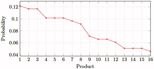
In total there are now 30 order pickers working per shift in the warehouse. Different from Gong and de Koster (2008) who assumed that all order pickers visit sequentially every storage location and thus follow the same picking route, we assume that the order picking area is zoned and each picker is responsible for picking products from his or her zone. This means that there is no overlap in picking routes between order pickers. Picked products are brought to a central depot location where they are sorted per customer order. Additionally, we assume small-sized orders (64% one product unit and 36% two product unit) and that every customer order can be fully picked in one zone. This allows us to study each zone in isolation. In Figure 6 the probability a product is ordered is shown for the products stored in the zone.

Figure 6. Expected demand distribution China online shopping warehouse.

Then, a single order picker is responsible for $N=16=2\cdot 4\cdot 2$ storage locations. The subsequent picking routes can be realized by adding additional cross-aisles to the order picking area. Each order picker has a traveling speed of 0.48 meter/second. The mean travel time side to side is $s_1=2$ seconds, the mean travel time within aisles between adjacent storage location is $s_2=2.50$ seconds, and the mean travel time between adjacent aisles is $s_3=9.60$ seconds. The average mean traveling times from the last storage location to the first pick location including the depot time is $s_0=63.0$ seconds for all the pickers. As a result, the total mean traveling time per cycle is $E(S)=182.2$ seconds. All the second moments for the traveling times are $s_i^2=0,i=0,1,2,3$. Finally, for all storage locations the mean picking time per product unit is $E(B_i)=1.51$ seconds and second moment of the picking time is $E(B_i^2)=3.82,i=1,\dots ,N$. In the rest of this section, we focus on one zone but the same conclusion can also be drawn for the other zones.

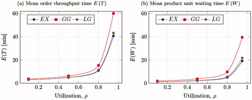
Figure 7 shows the mean order throughput time and mean product unit waiting time for the three picking strategies, for different system utilizations. The results were obtained after running the GA for which the parameters were identical as in Section 7.1. The run time of the algorithm was around 5 minutes per instance and around 500 generations were needed to find the best allocation. In Figure 7(a) the results for the mean order throughput time $E(T)$ are shown. The exhaustive strategy always achieves the lowest mean order throughput time, whereas the results of the locally-gated strategy are slightly above it. However, the globally-gated strategy performs significantly worse which shows that dynamically adding new customer orders to the picking cycle reduces the mean order throughput times considerably. For high arrival rates, the globally-gated strategy resembles a conventional batch picking process. In the cases of LG and EX where new customer orders can be included in the current picking cycle, a substantially better performance is obtained. From the results, it can be clearly seen that when the utilization increases, the mean order throughput times also increase. For the average mean product unit waiting time $E(W)=\frac{1}{\Lambda }{\sum }_{i=1}^N{\lambda }_{i}E(W_i)$ in Figure 7(b), similar conclusions can be drawn. On the other hand, comparing the results with the mean order throughput time it can be seen that the mean order throughput time is between 50 and 125% longer. This implies that when considering how long it takes to pick a customer order it is better to consider the order throughput time instead of product unit waiting time.

Figure 7. Results for China online shopping warehouse for different utilization ρ and the three picking strategies.

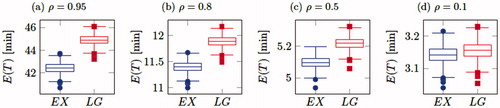
Figure 8 shows how much the mean order throughput time varies for several values of the utilization ρ for a randomly generated set of product allocations. We generated 3 000 different allocations, which also included the best allocation found in Figure 7, for which we calculated the mean order throughput time $E(T)$. We excluded the globally-gated strategy from this comparison, as $E(B_i)$, $i=1,\dots ,N$ is the same for every storage location, and therefore all product allocations have the same mean order throughput time. From the box plots it can been seen that the spread of mean order throughput times is around 3 minutes for the case where ρ is low, to a couple of seconds when ρ is high and that an approriate picking strategy can lead to significantly shorter order throughput times. In addition, the best storage allocation can improve the order throughput time by around 10% compared with the worst storage allocation. Finally, we tested the robustness of our results by perturbating the demand distribution and comparing the order throughput time of the allocations found by the GA each with a 1 000 random allocations. We found that changing up to 20% of the realizations of the demand distribution, the allocations found by the GA still provide the shortest order throughput times.

Figure 8. Box plots of mean order throughput times for 3000 different product allocations for various values of the utilization ρ.

8. Conclusion and further research

This article studied the order throughput time and product allocation in a milkrun picking system. This article is the first article order throughput times of multi-product unit orders in a milkrun picking system and provides better insights in the performance of the system and allows the effect of different product allocations to be studied. For three picking strategies; exhaustive, locally-gated, and globally-gated, we determined the average order throughput time of a customer order within the set of modelling assumptions. Afterwards, we proposed an optimization framework for product allocation in a milkrun picking system in order to minimize the average order throughput time. Our results showed that the average order throughput time in a milkrun order system can significantly vary based on the chosen product allocation and picking strategy. In particular, we found that the exhaustive strategy obtains the lowest mean order throughput time when travel times between storage locations are long compared with the picking times, whereas both gated strategies perform better in the opposite situation. In addition, for a real-world application we showeed that milkrun order picking reduces the order throughput time significantly in the case of high arrival rates compared with conventional batch picking. In addition, the best storage allocation can improve the order throughput time around 10% compared with the worst storage allocation.

Our results provide useful insights into the possible performance gain of a milkrun system compared with a traditional batch picking system. Moreover, it provides an understanding that, depending on the system and demand characteristics, different picking strategies will minimize the mean order throughput time. Short order throughput times are important for e-commerce companies that want to set their order cut-off times as late as possible while still guaranteeing that orders can be delivered next day or in some cases even the same day. Especially the latter case of same-day delivery, a milkrun system is very well suited. Examples are same-day grocery delivery companies or suppliers of consumer electronics as the company described in the real-world case.

The model and methods in this article lend themselves to further research. First, the model can be extended by including putaway and replenishment processes, similar as observed in a production setting. Other interesting topics are relaxing the assumption of an uncapacitated pick cart, investigating whether other or combinations of picking strategies can lead to increased picking performance, and multiple storage locations per product. Also, it can be worthwhile to investigate whether a local backward routing strategy, i.e., picking a product that arrived in the queue that just has been visited, might increase system performance. In addition, it is possible to further study a milkrun picking system with multiple pickers, where the order picking area is zoned and each picker is responsible for picking products from his/her zone. Interesting other research questions would be how many zones are required and how should products be allocated in order to minimize the order throughput time in the case where an order consists of demand for products located in multiple zones which all need to be send to single depot location. Finally, the model can be generalized for the analysis of different warehouse systems such as carousels or paternosters, but also for production systems and communication networks.

Additional information

Notes on contributors

J. P. van der Gaast

Notes on contributors

Jelmer Pier van der Gaast is a postdoc at the University of Groningen. He received his PhD in 2016 at the Erasmus University Rotterdam. His research interests include: warehouse operations, stochastic processes, and queueing theory. His research has been published in several journals including Transportation Science, Queueing Systems, and Computers & Operations Research.

René B. M. de Koster

René B. M. de Koster is a Professor of Logistics and Operations Management at Rotterdam School of Management, Erasmus University. His research interests are warehousing, terminal, and behavioral operations. He is an author/editor of eight books and over 150 papers in books and journals. He is guest lecturer at universities in Belgium, China, and South Africa. He is/was in the editorial boards of Operations Research, Journal of Operations Management, Transportation Science (SI editor), and other journals. He is a member of several international research advisory boards (including the European Logistics Association and BVL www.bvl.de). He is chairman of Stichting Logistica and founder of the Material Handling Forum (www.rsm.nl/mhf). His research has received several awards (IIE Transactions 2009, 2016; Journal of Operations Management finalist 2007; Academy of Management best paper finalist 2013).

Ivo J. B. F. Adan

Ivo J. B. F. Adan received his MSc and PhD in Mathematics from TU/e. Since 2011 he has been a Full Professor in Manufacturing Networks in the Department of Mechanical Engineering, TU/e, and was previously an Associate Professor in the Department of Mathematics and Computer Science. In 2001–2002 he was visiting professor at the Operations Research Department of the University of North-Carolina. In 2008-2011 he was also affiliated with the University of Amsterdam as a professor in Stochastic Operations Research. He serves on the editorial boards of Queuing Systems and Probability in the Engineering and Informational Sciences. Ivo Adan is a senior fellow of Eurandom and he is the research director of Beta, which is the national network of Operations Management and Logistics.

References

- Boon, M.A.A., van der Mei, R.D. and Winands, E.M.M. (2011) Applications of polling systems. Surveys in Operations Research and Management Science, 16(2), 67–82.
- Boon, M.A.A., van Wijk A.C.C., Adan, I.J.B.F. and Boxma, O.J. (2010) A polling model with smart customers. Queueing Systems, 66(3), 239–274.
- Bottani, E., Cecconi, M., Vignali, G. and Montanari, R. (2012) Optimisation of storage allocation in order picking operations through a genetic algorithm. International Journal of Logistics Research and Applications, 15(2), 127–146.
- Bozer, Y.A. and Ciemnoczolowski, D.D. (2013) Performance evaluation of small-batch container delivery systems used in lean manufacturing – Part 1: System stability and distribution of container starts. International Journal of Production Research, 51(2), 555–567.
- Ciemnoczolowski, D.D. and Bozer, Y.A. (2013) Performance evaluation of small-batch container delivery systems used in lean manufacturing — Part 2: Number of kanban and workstation starvation. International Journal of Production Research, 51(2), 568–581.
- De Koster, M.B.M., Le-Duc, T. and Roodbergen, K.J. (2007) Design and control of warehouse order picking: A literature review. European Journal of Operational Research, 182(2), 481–501.
- De Koster, M.B.M., van der Poort, E.S. and Wolters, M. (1999) Efficient order batching methods in warehouses. International Journal of Production Research, 37(7), 1479–1504.
- Emde, S. and Boysen, N. (2012) Optimally routing and scheduling tow trains for JIT-supply of mixed-model assembly lines. European Journal of Operational Research, 217(2), 287–299.
- Frazelle, E.H. (1990) Stock location assignment and order batching productivity. Ph.D. thesis, Georgia Institute of Technology, Atlanta, GA.
- Gademann, N. and van de Velde, S. (2005) Order batching to minimize total travel time in a parallel-aisle warehouse. IIE Transactions, 37(1), 63–75.
- Garfinkel, M. (2005) Minimizing multi-zone orders in the correlated storage assignment problem. PhD thesis, Georgia Institute of Technology, Atlanta, GA.
- Goldberg, D.E. and Lingle, R. (1985) Alleles, loci, and the traveling salesman problem, in Proceedings of the First International Conference on Genetic Algorithms and their Applications, Lawrence Erlbaum Associates, Publishers, pp. 154–159.
- Gong, Y. and de Koster, M.B.M. (2008) A polling-based dynamic order picking system for online retailers. IIE Transactions, 40(11), 1070–1082.
- Gong, Y. and de Koster, M.B.M. (2011) A review on stochastic models and analysis of warehouse operations. Logistics Research, 3(4), 191–205.
- Hanson, R. and Finnsgård, C. (2014) Impact of unit load size on in-plant materials supply efficiency. International Journal of Production Economics, 147(A), 46–52.
- Kilic, H.S. and Durmusoglu, M.B. (2013) A mathematical model and a heuristic approach for periodic material delivery in lean production environment. The International Journal of Advanced Manufacturing Technology, 69(5-8), 977–992.
- Kim, K.H. (1993) A joint determination of storage locations and space requirements for correlated items in a miniload automated storage-retrieval system. International Journal of Production Research, 31(11), 2649–2659.
- Korytkowski, P. and Karkoszka, R. (2016) Simulation-based efficiency analysis of an in-plant milk-run operator under disturbances. The International Journal of Advanced Manufacturing Technology, 82(5–8), 827–837.
- Kovács, A. (2011) Optimizing the storage assignment in a warehouse served by milkrun logistics. International Journal of Production Economics, 133(1), 312–318.
- Little, J.D.C. (1961) A proof of the queuing formulaL=λW. Operations Research, 9(3), 383–387.
- Mitchell, M. (1998) An Introduction to Genetic Algorithms. MIT Press, Cambridge, MA.
- Reeves, C. (2003) Handbook of Metaheuristics, pp. 55–82, Boston, MA: Springer Science & Business Media.
- Staab, T., Klenk, E., Galka, S. and Günthner, W.A. (2016). Efficiency in in-plant milk-run systems – The influence of routing strategies on system utilization and process stability. Journal of Simulation, 10(2), 137–143.
- Takagi, H. (1986) Analysis of Polling Systems. MIT Press, Cambridge, MA.
- Tsai, C.Y., Liou, J.J.H. and Huang, T.M. (2008) Using a multiple-GA method to solve the batch picking problem: Considering travel distance and order due time. International Journal of Production Research, 46(22), 6533–6555.
- Van den Berg, J.P. (1999) A literature survey on planning and control of warehousing systems. IIE Transactions, 31(8), 751–762.
- Van der Gaast, J.P., Adan, I.J.B.F. and de Koster, R.B.M. (2017) The analysis of batch sojourn-times in polling systems. Queueing Systems, 85(3), 313–335.
- Whitley, L.D., Starkweather, T. and Fuquay, D. (1989, June) Scheduling problems and traveling salesmen: The genetic edge recombination operator, in Proceedings of the Third International Conference on Genetic Algorithms, Vol. 89, pp. 133–140. Fairfax, Virginia. Morgan Kaufmann Publishers.
- Wolff, R.W. (1982) Poisson arrivals see time averages. Operations Research, 30(2), 223–231.
- Xiao, J. and Zheng, L. (2011) Correlated storage assignment to minimize zone visits for BOM picking. The International Journal of Advanced Manufacturing Technology, 61(5-8), 797–807.