Inequity-averse shelter location for disaster preparedness

Abstract

We study the problem of selecting a set of shelter locations in preparation for natural disasters. Shelters provide victims of a disaster both a safe place to stay and relief necessities such as food, water and medical support. Individuals from the affected population living in a set of population points go to, or are transported to the assigned open shelters. We aim to take both efficiency and inequity into account, thus we minimize a linear combination of: (i) the mean distance between opened shelter locations and the locations of the individuals assigned to them; and (ii) Gini’s Mean Absolute Difference of these distances. We develop a stochastic programming model with a set of scenarios that consider uncertain demand and disruptions in the transportation network. A chance constraint is defined on the total cost of opening the shelters and their capacity expansion. In this stochastic context, a weighted mean of the so-called ex ante and ex post versions of the inequity-averse objective function under uncertainty is optimized. Since the model can be solved to optimality only for small instances, we develop a tailored Genetic Algorithm (GA) that utilizes a mixed-integer programming subproblem to solve this problem heuristically for larger instances. We compare the performance of the mathematical program and the GA via benchmark instances where the model can be solved to optimality or near optimality. It turns out that the GA yields small optimality gaps in much shorter time for these instances. We run the GA also on Istanbul data to drive insights to guide decision-makers for preparation.

Keywords:

• Shelter location
• inequity aversion
• chance–constrained optimization
• disaster preparedness

1. Introduction

Although efficiency, e.g., minimizing total cost, is the major concern in commercial operations, equity is an essential requirement in humanitarian operations such as response services. Optimization problems addressing operational aspects should aim at providing equitable services to victims in order to make the suggested solutions acceptable. In the Operations Research literature, equity has been addressed in problems such as resource allocation, facility location, scheduling and transportation in various contexts such as bandwidth allocation in telecommunications; cost/benefit allocation in collaborative logistics; organ, blood, and drug allocation in health care; public facility location (Balcik et al., 2010), and hazardous material transportation (Gopalan et al., 1990). However, in humanitarian operations, models that address inequity-averseness have received relatively less attention. In this research, we aim to incorporate both efficiency and equity objectives into a stochastic facility location problem, namely choosing the locations of shelter facilities for preparedness against natural disasters.

In general, equity (often synonymously called fairness) aims at equal distribution of benefits or disutilities. For instance, in hazardous material transportion, Gopalan et al. (1990) calculate the risk associated with an accident for each district in a network as a disutility measure. Then for considering equity, they impose a limit on the difference in total risk between every pair of districts. In facility location problems, geographic equity of access to service facilities has been measured in different terms, usually based on the distances between demand points and assigned facilities (see the review articles by Karsu and Morton (2015) and Ogryczak (2000)). Maximizing the share of population covered within a pre-defined distance or travel time, or minimizing the maximum distance from demand points to facilities (Rawlsian approach) are examples of approaches commonly resorted to in facility location. On the other hand, mean absolute deviation and the Gini coefficient have been utilized in the economics literature for assessing income inequity among individuals. In this study, we develop a model that incorporates measures of equity from the economics literature, to balance efficiency and equity in shelter location decisions under uncertainties concerning demand locations, demand amounts, and road network accessibility.

We study the problem of selecting the locations of shelters to be established as a preparation step for possible natural disasters. Following a disaster, shelters are often provided by organizations or governmental agencies to gather the victims into a safe temporary living space and deliver essential relief services to them, such as food, water, medicine, etc. In case of a disaster, persons from an affected population at different locations go to or are transported to the assigned opened shelters. Informing the people before a disaster about which shelter they are assigned to, as a preparedness measure, saves precious time after a disaster, and helps the planning activities. On the side of an individual, the disutility of the travel to the shelter is expressed by the distance to the assigned shelter. Our goal is to minimize a measure derived from individual distances that takes both efficiency and inequity into account. Efficiency is defined by the mean distance traveled by an individual to reach the assigned shelter location, and inequity is measured as Gini’s Mean Absolute Difference of the distances.

Since it is not clear in advance where the disaster will strike and which population nodes it will affect and to what extent, we use a stochastic model with a set of possible disaster scenarios. Demand, affected population, and traversable road distances between population nodes and facility locations depend on the scenarios. In order to also consider budget limitations, we use a chance constraint. This constraint ensures that with a given minimum probability near to unity, the total monetary cost of opening the shelters and expanding their capacities based on the realized demands after the disaster does not exceed the given budget. In the context of the mentioned scenario-based representation of the random demand, the chance constraint will be expressed by its deterministic equivalent. Thus, it requires that the total cost must be within the limit of the given budget in a pre-specified (high) percentage of the scenarios. The chosen percentage represents the service level. To the best of our knowledge, a model with chance constraints has not been studied before in the context of shelter location in disaster logistics. To solve our problem, we use a modified genetic algorithm and compare its performance against a stochastic program solved by the Cplex solver. Finally, we solve our problem on real data obtained on the Kartal district in Istanbul to yield insights for decision makers.

The rest of this article is organized as follows. The next section provides an overview of related literature. In Section 3, we describe the problem and introduce the Mixed-Integer Programming (MIP) model for the problem. The genetic algorithm is explained in Section 4. In Section 5, we describe the generation of benchmark instances and the Istanbul data and discuss our experimental results. Finally, we present concluding remarks in Section 6.

2. Related literature

2.1. Inequality measurement under uncertainty

A general survey on inequity-averse optimization has recently been given by Karsu and Morton (2015). Therein, also some papers dealing with humanitarian logistics applications are reviewed. Nevertheless, these approaches are restricted to a deterministic framework. In Gutjahr and Nolz (2016), several types of objective functions for optimization approaches to humanitarian logistics are discussed, in particular also equity. In this survey, it is observed that in this area, articles dealing with equity are rather scarce and focused on the deterministic case.

In the literature on decision theory, on the other hand, the issue of inequity measurement under uncertainty has found explicit consideration. For the purpose of our current investigation, four articles are especially important. Ben-Porath et al. (1997) discuss the conceptual difficulty of equity quantification in a context of uncertainty, a difficulty which is mainly caused by the contrast between ex ante inequity and ex post inequity: In the case of uncertainty, it is not clear whether one should strive for equity from the perspective before a random or uncertain event has happened, or from the perspective after uncertainty has been resolved. As a solution concept, the authors propose the so-called min-of-means functionals and study their properties from an axiomatic point of view. Gajdos and Maurin (2004) show that already a very restricted set of reasonable axioms rules out both pure ex ante inequity measures and pure ex post inequity measures as meaningful quantifications of inequity under uncertainty. Chew and Sagi (2012) propose a one-parameter extension of the Generalized Gini Mean as an inequity measure under uncertainty, and investigate it in an axiomatic framework. New theoretical findings, again from an axiomatic perspective, are provided in Fleurbaey et al. (2015). All these works, however, aim at economic theory, not optimization. To the best of our knowledge, the current article is the first one that uses a decision-theoretic measure for inequity under uncertainty as an objective function of an applied optimization problem, and shows how the resulting optimization model can be solved computationally.

2.2. Inequality-averse optimization in humanitarian operations

In a deterministic context, the humanitarian logistics literature has represented equity either by including an equity-related measure among multiple objectives or by adding constraints to ensure fair distribution of resources and access to facilities. Holguín-Veras et al. (2013) discuss objective functions for post-disaster humanitarian logistics models and argue that nonlinear deprivation cost functions representing the suffering of people due to lack of goods and services should be used. Considering increments of deprivation levels in a model introduces a trend to more equitable relief distribution plans. Gralla et al. (2014) suggest that prioritization of commodities and delivery locations can serve as a means to promote equity, and evaluate this objective in relation to other measures by interviewing field experts in humanitarian logistics. A multi-objective stochastic program is proposed by Bozorgi-Amiri et al. (2013), where minimizing the sum of the maximum shortages is one of the objectives. Afshar and Haghani (2012) add constraints to their model to ensure equity. For instance, the amount of each commodity delivered to each demand point up to a time point must constitute at least a certain fraction of the total amount.

Vitoriano et al. (2011) use a goal programming approach to deal with eight objective functions, including an equity objective. Ortuño et al. (2011) incorporate equitable distribution of goods in a lexicographical goal programming formulation for humanitarian aid distribution. Ransikarbum and Mason (2016) adopt a goal programming method to relief supply distribution and early-stage network restoration, addressing equity by maximizing the minimum percentage of satisfied demand. Similar approaches have been pursued in the works by Tzeng et al. (2000), Lin et al. (2011), and Huang et al. (2012). Eisenhandler and Tzur (2016) address the problem of an efficient and fair distribution of perishable goods from food suppliers to welfare agencies serving people in need of food. Gutjahr and Fischer (2018) show that the deprivation cost concept, which has recently been proposed to derive suitable objective functions for humanitarian logistics models, can (and should) be extended to take the equity issue into account. The two last-mentioned works come close to our present article insofar as they also use the Gini index to quantify inequity, but both approaches are restricted to a deterministic situation.

2.3. Shelter location problems

As defined by the International Federation of Red Cross shelters are safe areas that provide accommodation, climate protection, food and medical care for victims of a disaster. Moreover, they protect the population from possible threats that might arise later on. Selection of suitable sites for the shelters is of critical importance, as it affects the performance of an evacuation plan (Kongsomsaksakul et al., 2005). Determining shelter locations considering evacuees’ allocation is now being recognised as a critical decision to successful disaster management, and has gained significant attention among researchers in recent years. A notable number of studies have been proposed for shelter and evacuation planning and are discussed in Bayram (2016).

Uster and Dalal (2017) introduced an integrated emergency network design problem in which three levels exist. They decided on the locations of supply facilities, distribution centers and shelters, and allocation of demands and disaster relief goods to those shelters. They adopted two objective functions: one minimizing total cost; and the other one minimizing the maximum distance that a disaster victim should travel to reach the assigned shelter. They solve this deterministic multi-objective optimization problem by the $ϵ$-constraint method and Benders decomposition.

Some researchers have taken advantage of fuzzy set theory to deal with uncertainty in shelter location problems. Trivedi and Singh (2017) consider multi-objective capacitated shelter location and demand assignment. They represent uncertainty with fuzzy sets. As objective functions, their model minimizes total distance, risk associated with locations, number of sites and uncovered demand, and simultaneously maximizes site suitability score and its degree of public ownership. Another study that adopts multi-objective modeling for evacuation planing is Coutinho-Rodrigues et al. (2012). They consider six objective functions including minimizing total traveled distance, risks related to paths and shelters, number of shelters and total distance to the nearest medical care center. They also define backup paths for demand to shelter allocation in case the main paths fail after the disaster. They test the proposed model at the central area of Coimbra, Portugal. Wang et al. (2016) introduced a bi-objective model that maximizes both road and shelter reliability, claiming these two objectives are conflicting. They solve their deterministic model by the non-dominating sorting genetic algorithm (NSGA-II). As a case study they applied their model on Wenzhou City in Zhejiang Province, China.

Although the vast majority of the existing evacuation planning models assumes system-optimal (cooperative) behavior, a few researchers focus on selfish (noncooperative) behavior, which is more probable during a large evacuation. Ng et al. (2010) introduced a hybrid bilevel model that aims to capture a more realistic victim behavior during the disaster. In designing an evacuation plan, there is a tradeoff between assigning evacuees to the nearest open shelter or using an optimal strategy for the assignments. To address this tradeoff, Bayram et al. (2015) consider that evacuees can only be assigned to an open shelter within a range specified by a tolerance from the distance to the closest shelter. Kılcı et al. (2015) study shelter location by considering equity aspects in their model. Based on Turkish Red Crescent guidelines, they assign priority weights to potential sites and maximize the minimum weight of open shelter areas among selected sites. They include constraints to limit maximum distances, minimum utilization of individual shelter sites and utilization differences between selected sites.

Li et al. (2011) consider two types of shelters, permanent and temporary shelters, and apply two-stage stochastic programming for capturing uncertainty. Permanent shelters’ locations and their capacities are treated as first-stage decisions, resource allocation and temporary shelter locations are considered as the second-stage decisions.

2.4. Stochastic facility location problems in humanitarian operations

The facility location problem for disaster preparedness has been modeled by stochastic programs, especially by two-stage stochastic programming, in many studies within the past decade. Grass and Fischer (2016) present a comprehensive review on two-stage stochastic programming in disaster management. A recent survey on facility location problems that are related to humanitarian logistics, covering also stochastic models, is provided by Boonmee et al. (2017). Hoyos et al. (2015) provide a literature review on studies in disaster management that apply Operations Research models with a stochastic component, including those related to facility location.

Rawls and Turnquist (2010) introduce a two-stage stochastic program where the first stage decisions are on opening warehouses and amount of items to be pre-positioned. Uncertainty in demand amounts, arc capacities and survival probabilities of the pre-positioned items are represented by a set of discrete scenarios. Verma and Gaukler (2015) provide a two-stage stochastic programming model of pre-disaster facility location that considers the damage intensity as a random variable. Döyen et al. (2012) propose a two-echelon facility location model where uncertain transportation time and demand values are represented by discrete scenarios. Galindo and Batta (2013) model the possible destruction of supply points during the disaster event and Paul and MacDonald (2016) model uncertainties such as facility damage and casualty losses as a function of the magnitude of an earthquake while deciding on the location and capacities of distribution centers. Noyan (2012) utilizes Conditional Value-at-Risk (CVaR) as a risk measure in a stochastic model of facility location and material flow. Tricoire et al. (2012) and Rath et al. (2015) propose two-stage programming models for humanitarian location/routing problems under multiple objectives.

Hu et al. (2016) decide on both reinforcement of road networks and buildings, and facility location with the objectives of minimizing the budget and the risk-induced penalties. Bayram and Yaman (2017) consider the uncertainty in road network, evacuation demand and disruption in shelters by a set of discrete scenarios. They devise a Benders decomposition approach to solve the stochastic shelter location and evacuee allocation problem, with minimizing expected total evacuation time as their objective. In a very recent study, Elçi and Noyan (2018) consider a location-allocation problem for disaster preparedness under demand and network uncertainty. They propose a two-stage stochastic programming model with a chance constraint, which in the first stage decides on the relief facilities’ locations and their inventory levels. In the second stage, the allocation of relief supplies are made for each scenario. They also define two types of second-stage problems; one problem allows supply shortage and the other one enforces satisfaction of all the demands. To model the decision maker’s risk preferences on total random cost, they use CVaR as a risk measure in the objective function. A Benders decomposition–based branch-and-cut algorithm is devised to solve the problem efficiently.

In Renkli and Duran (2015) and Ukkusuri and Yushimito (2008), locations for prepositioning inventory are selected by a path-reliability approach. Ukkusuri and Yushimito (2008) aim at maximizing the probability of sending materials to demand points, whereas Renkli and Duran (2015) constrain the probability of meeting the demand of an item to be at least a specified amount. Kulshrestha et al. (2011) develop a bilevel model under demand uncertainty and solve it by robust optimization. At the upper level, authorities decide about the number, capacity and locations of shelters and at the lower level, the evacuees choose which shelter to go to.

In most of these studies discussed above, the generation of the scenarios has not been addressed explicitly and the statistical dependency between the scenarios has also not been an explicit topic. Salman and Yücel (2015) suggest a systematic method to generate correlated road network scenarios based on the vulnerability level of the network edges and their spatial closeness while locating emergency response centers. In our current study, we generate a sample of scenarios with uncertain demand and travel times resulting from correlated probabilistic failures of road links based on the link failure dependency model in Yücel et al. (2018), which is explained in Section 5.2.1.

Very few articles on stochastic facility location for humanitarian purposes address the equity issue. Rezaei-Malek and Tavakkoli-Moghaddam (2014) propose a two-stage stochastic programming model for pre-positioning of relief goods, taking account of equity by means of a fairness level constraint. Noyan et al. (2015) determine locations and capacities of relief distribution points by a two-stage stochastic programming model, optimizing the expected total accessibility with a penalty for inequitable solutions. The maximum proportion of unsatisfied demand is used as an equity measure. As far as we know, the combination of a stochastic programming model with the Gini inequity measure, as suggested in the present article, is not only new in the humanitarian logistics literature in particular, but in the optimization literature in general.

3. Problem definition

Let J be a set of Candidate Locations (CLs) for the facilities, which we call “shelters” although the model admits a more general interpretation, e.g., one where the facilities are local distribution centers, medical units, etc. Let $\left|J\right|=m$. A set K of Population Nodes (PNs) is given, where $\left|K\right|=n$. PN $k\in K$ has w_k inhabitants. To capture the uncertainty, we define a finite set S of scenarios, where each scenario s has a certain occurrence probability, p_s. Depending on where the disaster strikes and how severe it is, a demand of $b_k^s$ $(0\le b_k^s\le w_k)$ occurs in PN k. Here we consider demand as a portion of the population. Thus, $b_k^s$ can be interpreted as the number of people from PN k who have to be transported to a shelter under scenario s, but the model is general enough to also allow other interpretations. In scenario s, the demand vector is $(b_1^s,\dots ,b_n^s)$. Furthermore, the distance matrix is $D=(d_{kjs})$, where d_kjs is the (network) distance between PN k and CL j in scenario s. Note that in view of possible road failures, the distance between two points depends on the scenario.

Each CL j has a pre-defined capacity c_j. Since assignments are independent of scenarios, the pre-decided demand allocations to CL j can exceed the capacity of the facility. Whenever this happens, a recourse action takes place where the facility is expanded at the price of a unit expansion (penalty) cost ${\eta }_j$, in order to be able to accommodate all assigned victims. The decision on expansion differs for each scenario, as demands are dependent on the scenarios. Opening a shelter in CL j incurs an establishment cost f_j, independent from the scenarios. A budget C limits the total cost, i.e., the sum of all establishment costs and expansion costs. If the budget is exceeded, then there must be unassigned individuals. To maintain a certain service level α, the total cost must not exceed the budget with probability of at least α.

The location decisions are represented by a binary vector $x=(x_j)$, where x_j = 1 if a shelter is opened at CL j and x_j = 0 otherwise, for all $j\in J$. The assignment of the affected individuals in PN k to the open shelter at location j is shown by variable y_kj, where y_kj takes the value 1 if we assign PN k to the open shelter j, otherwise it takes the value 0, for all $k\in K,j\in J$. Note that we consider the assignment of PNs to CLs as a decision that is made in a pre-disaster stage, contrary to some other stochastic models for disaster response that assume that the assignment of individuals to shelters is done only after the disaster, i.e., after uncertainty has been resolved and all demands are known. For many cases, the latter is a reasonable assumption with the potential to increase the efficiency of the solution by letting the assignment decision depend on the actual random scenario. However, there are other situations where a pre-assignment of people to shelters is advantageous: Knowing the assignments already in the preparedness stage allows the planner to tell (and even train) the individuals which shelter they should go to in case of a disaster, and by which evacuation path. This may be especially important for children and old people. It will facilitate a faster evacuation after the disaster and avoid chaos. In addition, it is often the case that telecommunication infrastructure is disrupted by the disaster, which will delay the disaster relief operations and may lead to very undesirable consequences if an assignment to shelters depends on information that is only available after the disaster has struck. Therefore, we assume a pre-disaster allocation of people to shelters in the current work.

Other types of models would be obtained by the assumption that the victims of the disaster choose the shelters themselves, based on individual decisions. Their choice could be as simple as to seek the nearest opened shelter (Nearest Assignment, NA), or it could also take more involved considerations into account such as a preference for opened shelters that are expected not to be congested; the latter would lead to a User Equilibrium (UE) model (cf. Gutjahr and Dzubur (2016)). The downside of the NA approach may be higher costs for capacity expansion. A UE model, on the other hand, seems to be more appropriate for situations where the damage to the infrastructure is less severe, as under a largely disrupted infrastructure, people may not have enough information to make a user choice based on sound congestion estimates. For these reasons, we do not consider the last-mentioned types of models here.

In the objective function of the problem we want to account for both efficiency and equity. Different quantifications of equity have been proposed in the literature (Marsh and Schilling, 1994; Karsu and Morton, 2015) These approaches include, among others, the Rawlsian (i.e., minimum or maximum) measure, the lexicographic extension of the Rawlsian measure, the mean deviation, the variance, the range, the Gini index (also called Gini coefficient), or Hoover’s concentration index. In the present work, we have decided to adopt the Gini index for two reasons. First, this index has been extensively used in economics to represent inequality and will therefore be easily understood by managers with an education in economics. Second, the index has favorable theoretical properties, as scale invariance with respect to multiplication by positive constants, symmetry (switching two individuals will not change the index), and validity of the Pigou–Dalton Principle of Transfers, which basically says that if a small amount of a good is transferred from an individual owning more to an individual owning less, then the inequality index will improve or at least not become worse. Whereas the Gini index is typically formulated for benefits as wealth or income, we need it for disadvantages or costs. The Gini index for costs (in our case: distances) $d^{(i)}$ $(i=1,\dots ,N)$ of N individuals can be defined analogously as the Gini index for benefits as (1) $$G=\frac{1}{2N}\frac{{\sum }_{i=1}^N{\sum }_{j=1}^N|d^{\left(i\right)}-d^{\left(j\right)}|}{{\sum }_{i=1}^N{d}^{\left(i\right)}}$$(1) (Drezner et al., 2009; Yitzhaki and Schechtman, 2013). The minimum value of G is zero (perfect equity), the maximum value is one (extreme inequity). However, we do not use the Gini index itself as an objective function, as minimization of the Gini index alone would result in equitable, but very inefficient solutions, as argued in Drezner et al. (2009). Therefore, what we need as an objective function is an inequity-averse aggregation function (taking also efficiency into account) rather than an inequity measure alone. For this reason, we replace the Gini index G for distances by a linear combination $\mathcal{I}=\mu +\lambda \Delta$. Therein, $\mu =(1/N){\sum }_{i=1}^N{d}^{(i)}$ is the mean distance, and $\Delta =2\mu G$ is Gini’s Mean Absolute Difference of the distances.

The choice of a linear combination of the efficiency measure μ and the equity measure Δ as the objective is intuitively plausible, and the decision to take $\Delta =2\mu G$ rather than G itself as the equity measure is easily explained by the requirement that both measures have to be expressed in the same units if they are to be combined to a weighted sum. (Note that G is dimensionless.) However, there are deeper reasons justifying the choice of $\mathcal{I}=\mu +\lambda \Delta$, which can be elucidated by the theory of symmetric comonotonically linear functionals from the inequity measurement literature, see Ben-Porath et al. (1997). (Details can be found in an online supplement to this article.) From this theory, it also follows that the weight factor λ should be within the range $0\le \lambda \le 1/2$.

To represent uncertainty in our problem, we follow the approach in Ben-Porath et al. (1997). The key difficulty treated therein, the contrast between ex ante inequity and ex post inequity, can be stated in formal terms as follows: Suppose we have an inequity measure $\mathcal{I}(f)$ assigning to each vector ${(f(i))}_{i\in I}$ of costs of all individuals $i\in I$ a real number, and let f(s, i) denote the cost of individual i under random scenario s. Then it is not clear whether $\mathcal{I}(E[f(s,i)])$ or $E([\mathcal{I}(f(s,i))]$ should be optimized, where $\mathcal{I}$, acting on i, is the given inequity measure, and E, acting on s, is the mathematical expectation. Should we try to minimize the inequity of the expected outcome (ex ante consideration), or rather the expected inequity of the outcome (ex post consideration)?

To see the difference between the two criteria, consider the following example from Ben-Porath et al. (1997). Let us compare the three “social policies” f, g, and h below, where a social policy f is a function f(s, i) assigning costs to scenarios and individuals as above. In the example, two scenarios s and t with equal probabilities 0.5 and two individuals a and b are considered: $$\begin{array}{ccc}f& a& b\\ s& 0& 0\\ t& 1& 1\end{array}\hspace{1em}\hspace{1em}\begin{array}{ccc}g& a& b\\ s& 0& 1\\ t& 1& 0\end{array}\hspace{1em}\hspace{1em}\begin{array}{ccc}h& a& b\\ s& 0& 1\\ t& 0& 1\end{array}$$

The ex ante inequity perspective is indifferent with respect to the social policies f and g, as they entail the same expected cost of 0.5 for each of the two individuals, whereas it prefers f and g over the social policy h, which entails unequal expected costs of zero and one for individual a and b, respectively. The ex post inequity perspective, on the contrary, prefers f over both g and h, since f leads with probability one to a final overall state of equity, whereas g and h, between which the ex-post perspective is indifferent, result with probability one in a final overall state of inequity. Roughly summarizing, we can say that ex ante optimizes equity of chances, whereas ex post optimizes the chance of equity. It is not obvious which criterion is more appropriate in humanitarian logistics. On the one hand, humanitarian organizations would certainly not like to see big differences in the well-being and safety of victims after a disaster (ex post consideration). On the other hand, using exclusively the ex post criterion may discourage private or communal initiatives to protect against the consequences of disasters in advance by own efforts.

Ben-Porath et al. (1997) define a broad class of “reasonable” inequity measures taking both ex ante inequity and ex post inequity into account. A special case are weighted means of $\mathcal{I}(E[f(s,i)])$ and $E[\mathcal{I}(f(s,i))]$. This is the approach we follow here. As shown in Gajdos and Maurin (2004) (see Theorem 9), it is arguable from theoretical reasons that the two weights are chosen as equal. Therefore, in this article, we shall mainly choose: (2) $$\frac{1}{2}\mathcal{I}(E[f(s,i)\left]\right)+\frac{1}{2}E\left[\mathcal{I}\right(f(s,i)\left)\right],$$(2) as the objective. Based on the inequity-averse aggregation function $\mathcal{I}(d)=\mu (d)+\lambda \Delta (d)$, where d is the vector of all distances from individuals to assigned opened shelters, we specify now the objective functions for the ex ante and for the ex post case, respectively. The objective function for the combined case results as the weighted mean (2).

Ex ante problem: First of all, we compute the expected distance to be traversed by an inhabitant of PN k. With the defined notation, in scenario s, an inhabitant i of PN k has a probability of $b_k^s/w_k$ to be affected by the disaster. If (s)he is affected by the disaster, (s)he faces a distance of $d_{ks}=\sum _{j\in J}{y}_{kj}{d}_{kjs}$ to the assigned shelter. This is correct because we make sure that every population node is assigned only to one shelter. Therefore, the expected distance for an arbitrary person from PN k is ${\overline{d}}_k=\sum _{s\in S}{p}_s·(b_k^s/w_k)·d_{ks}.$ There are $N=\sum _{k\in K}{w}_k$ individuals in total. The Gini index of the values ${\overline{d}}_k$ (note that each value ${\overline{d}}_k$ has to be taken with multiplicity w_k for the w_k inhabitants of PN k) can easily be computed, using representation (1): $$\begin{array}{c}G=\frac{1}{2N}·\frac{\sum _{k\in K}\sum _{k\prime \in K}{w}_k{w}_{k\prime }|{\overline{d}}_k-{\overline{d}}_{k\prime }|}{\sum _{k\in K}{w}_k{\overline{d}}_k}\\ =\frac{1}{2N}·\frac{\sum _{k\in K}\sum _{k\prime \in K}\left|\sum _{s\in S}{p}_s\left(w_{k\prime }{b}_k^s\sum _{j\in J}{y}_{kj}{d}_{kjs}-w_k{b}_{k\prime }^s\sum _{j\in J}{y}_{k\prime j}{d}_{k\prime js}\right)\right|}{\sum _{k\in K}\sum _{s\in S}\sum _{j\in J}{p}_s{b}_k^s{y}_{kj}{d}_{kjs}}.\end{array}$$

Since the mean μ of the values ${\overline{d}}_k$ (taken with their multiplicities w_k) is $$\frac{1}{N}\sum _{k\in K}\sum _{s\in S}\sum _{j\in J}{p}_s{b}_k^s{y}_{kj}{d}_{kjs},$$ we get the following formula for the objective function (to be minimized) of the ex ante problem: (3) $$\begin{array}{l}{F}_{\mathit{\text{ante}}}=\mu +2\lambda \mu G=\frac{1}{N}\sum _{k\in K}\sum _{s\in S}\sum _{j\in J}{p}_s{b}_k^s{y}_{kj}{d}_{kjs}\\ +\frac{\lambda }{N^2}\sum _{k\in K}\sum _{k\prime \in K}\left|\sum _{s\in S}{p}_s\left(w_{k\prime }{b}_k^s\sum _{j\in J}{y}_{kj}{d}_{kjs}-w_k{b}_{k\prime }^s\sum _{j\in J}{y}_{k\prime j}{d}_{k\prime js}\right)\right|.\end{array}$$(3)

Ex post problem: Now we have to start with the computation of the Gini index (and of the inequity-averse aggregation function $\mathcal{I}(d)$) for a fixed scenario s. For a given scenario s, we reduce each PN k to those $b_k^s$ inhabitants that are affected by the disaster, and disregard the remaining $w_k-b_k^s$ inhabitants. We do not take these inhabitants into account since we want to judge equity only among those that are candidates for actions, i.e., assignments to shelters. This is possible in the ex post framework, since after scenario realization, it is already known who has been affected by the disaster and who has not. Let $N{\prime }_s=\sum _{k\in K}{b}_k^s$ be the total number of affected people in scenario s. Then, with d_ks as in the ex ante case, and again considering multiplicities (this time by the number of affected individuals instead of the number of all individuals), we get: $$G^s=\frac{1}{2N{\prime }_s}·\frac{\sum _{k\in K}\sum _{k\prime \in K}{b}_k^s{b}_{k\prime }^s|d_{ks}-d_{k\prime s}|}{\sum _{k\in K}{b}_k^s{d}_{ks}},\hspace{1em}s\in S.$$

Since the mean μ of the distances (considering their multiplicities) is $${\mu }^s=\frac{1}{N{\prime }_s}\sum _{k\in K}{b}_k^s{d}_{ks}(s\in S),$$$$the objective function of the ex post problem results by taking the expected value over the random scenarios as (4) $$\begin{array}{c}{F}_{\mathit{\text{post}}}=E[{\mu }^s+2\lambda {\mu }^s{G}^s]=\sum _{s\in S}{p}_s\frac{1}{N{\prime }_s}\sum _{k\in K}\sum _{j\in J}{b}_k^s{y}_{kj}{d}_{kjs}\\ +\lambda \sum _{s\in S}{p}_s\frac{1}{N{\prime }_s^2}\sum _{k\in K}\sum _{k\prime \in K}{b}_k^s{b}_{k\prime }^s|\sum _{j\in J}{y}_{kj}{d}_{kjs}-\sum _{j\in J}{y}_{k\prime j}{d}_{k\prime js}|.\end{array}$$(4)

Both the ex ante and the ex post problem can be cast into MIP formulations, as it will be shown in the next subsection. For example, the ex ante problem can be linearized by defining: $${\tau }_{k,k\prime }=\sum _{s\in S}{p}_s\left(w_{k\prime }{b}_k^s\sum _{j\in J}{y}_{kj}{d}_{kjs}-w_k{b}_{k\prime }^s\sum _{j\in J}{y}_{k\prime j}{d}_{k\prime js}\right),$$ and introducing the auxiliary variables ${\tau }_{k,k\prime }^{+}=\max ({\tau }_{k,k\prime },0)$ and ${\tau }_{k,k\prime }^{-}=\max (-{\tau }_{k,k\prime },0)$.

3.1. Formulation of the model

We are now in the position to present the suggested MIP models. All that is still missing is the chance constraint, expressing the condition that with at least a certain pre-specified probability α, the solution remains feasible even after shelter expansions, i.e., $Pr(\text{total}\text{cost}\le C)\ge \alpha$. Since randomness is represented in our model by the possible scenarios $s\in S$ with assigned probabilities p_s, the chance constraint takes the form $\sum _{s\in S}{p}_s{z}_s\ge \alpha$, where z_s is the indicator variable for the event that the total cost in scenario s is smaller or equal to the budget C. The formulations below give the deterministic equivalents of our chance-constrained stochastic programs. Table 1 lists the decision variables of the models.

Table 1. Decision variables.

Notation	Description	Variable type
xj	1 if CL j is opened, 0 otherwise	Binary
ykj	1 if all individuals in PN k are assigned to CL j, 0 otherwise	Binary
zs	1 if total cost meets the budget in scenario s, 0 otherwise	Binary
tjs	Amount of exceeded demand assigned to CL j in scenario s	Continuous

Ex ante problem: (5) $$\min \mu +2\lambda \mu G=\frac{1}{N}\sum _{k\in K}\sum _{s\in S}\sum _{j\in J}{p}_s{b}_k^s{y}_{kj}{d}_{kjs}+\frac{\lambda }{N^2}\sum _{k\in K}\sum _{k\prime \in K}({\tau }_{k,k\prime }^{+}+{\tau }_{k,k\prime }^{-}),\hspace{1em}$$(5) (6) $${\tau }_{k,k\prime }^{+}-{\tau }_{k,k\prime }^{-}=\sum _{s\in S}{p}_s\left(w_{k\prime }{b}_k^s\sum _{j\in J}{y}_{kj}{d}_{kjs}-w_k{b}_{k\prime }^s\sum _{j\in J}{y}_{k\prime j}{d}_{k\prime js}\right)\forall k,k\prime \in K,$$(6) (7) $$y_{kj}\le x_j\hspace{1em}\hspace{1em}\forall k\in K,j\in J,$$(7) (8) $$\sum _{j\in J}{y}_{kj}=1\hspace{1em}\hspace{1em}\forall k\in K,$$(8) (9) $$\sum _{k\in K}{b}_k^s{y}_{kj}\le t_{js}+c_j\hspace{1em}\hspace{1em}\forall j\in J,s\in S,$$(9) (10) $$\sum _{j\in J}{f}_j{x}_j+{\eta }_j{t}_{js}\le C+M_0(1-z_s)\hspace{1em}\hspace{1em}\forall s\in S,$$(10) (11) $$\sum _{s\in S}{p}_s{z}_s\ge \alpha ,$$(11) (12) $$\begin{array}{l}{x}_j\in \{0,1\}\hspace{1em}\forall j\in J,\hspace{1em}{z}_s\in \{0,1\}\hspace{1em}\forall s\in S,\hspace{1em}\\ y_{kj}\in \{0,1\}\hspace{1em}\forall k\in K,j\in J,\hspace{1em}\\ t_{js}\ge 0\hspace{1em}\forall j\in J,s\in S,\end{array}$$(12) (13) $${\tau }_{k,k\prime }^{+},{\tau }_{k,k\prime }^{-}\ge 0\hspace{1em}\hspace{1em}\forall k,k\prime \in K,$$(13)

To reformulate the objective function in linear terms, we introduced auxiliary variables ${\tau }_{k,k\prime }^{+}$ and ${\tau }_{k,k\prime }^{-}$ as discussed above and added constraints (6). Constraint (7) ensures that a PN can only be served by an opened shelter. Constraint (8) guarantees that each PN is assigned to exactly one shelter. Constraint (9) calculates the exceeded capacity for each CL in each scenario. Constraint (10) defines the indicator variable z_s for the satisfaction of the budget constraint in scenario s. If we meet the budget in scenario s, then z_s has no reason to become zero; otherwise, z_s will be zero. Our chance constraint (11) imposes that the budget should be met with probability at least α. Finally, the large number M₀ can be replaced by $\sum _{j\in J}(f_j+{\eta }_j(N-c_j))$.

Ex post problem: (14) $$\min \sum _{s\in S}\sum _{k\in K}\sum _{j\in J}\frac{1}{N{\prime }_s}{p}_s{b}_k^s{y}_{kj}{d}_{kjs}+\lambda \sum _{s\in S}{p}_s\frac{1}{N{\prime }_s^2}\sum _{k\in K}\sum _{k\prime \in K}{b}_k^s{b}_{k\prime }^s({\rho }_{kk\prime s}^{+}+{\rho }_{kk\prime s}^{-}),\hspace{1em}$$(14) (15) $$\text{s.t.}{\rho }_{kk\prime s}^{+}-{\rho }_{kk\prime s}^{-}=\sum _{j\in J}{y}_{kj}{d}_{kjs}-\sum _{j\in J}{y}_{k\prime j}{d}_{k\prime js}\hspace{1em}\forall s\in S,k,k\prime \in K,$$(15) (16) $${\rho }_{kk\prime s}^{+}{\rho }_{kk\prime s}^{-}\ge 0\hspace{1em}\forall k,k\prime \in K,s\in S,$$(16) constraints (7)(7) $$y_{kj}\le x_j\hspace{1em}\hspace{1em}\forall k\in K,j\in J,$$(7) –(12)(12) $$\begin{array}{l}{x}_j\in \{0,1\}\hspace{1em}\forall j\in J,\hspace{1em}{z}_s\in \{0,1\}\hspace{1em}\forall s\in S,\hspace{1em}\\ y_{kj}\in \{0,1\}\hspace{1em}\forall k\in K,j\in J,\hspace{1em}\\ t_{js}\ge 0\hspace{1em}\forall j\in J,s\in S,\end{array}$$(12) ,where ${\rho }_{kk\prime s}^{+}$ and ${\rho }_{kk\prime s}^{-}$ are three-indexed non-negative auxiliary variables that help us to make the objective function linear.

Combined problem: (17) $$\begin{array}{l}\min \gamma \left(\frac{1}{N}\sum _{k\in K}\sum _{s\in S}\sum _{j\in J}{p}_s{b}_k^s{y}_{kj}{d}_{kjs}+\frac{\lambda }{N^2}\sum _{k\in K}\sum _{k\prime \in K}({\tau }_{k,k\prime }^{+}+{\tau }_{k,k\prime }^{-})\right)\\ +(1-\gamma )(\sum _{s\in S}\sum _{k\in K}\sum _{j\in J}\frac{1}{N{\prime }_s}{p}_s{b}_k^s{y}_{kj}{d}_{kjs}+\lambda \sum _{s\in S}{p}_s\frac{1}{N{\prime }_s^2}\sum _{k\in K}\sum _{k\prime \in K}{b}_k^s{b}_{k\prime }^s({\rho }_{kk\prime s}^{+}+{\rho }_{kk\prime s}^{-})),\end{array}$$(17) s.t. constraints (6)(6) $${\tau }_{k,k\prime }^{+}-{\tau }_{k,k\prime }^{-}=\sum _{s\in S}{p}_s\left(w_{k\prime }{b}_k^s\sum _{j\in J}{y}_{kj}{d}_{kjs}-w_k{b}_{k\prime }^s\sum _{j\in J}{y}_{k\prime j}{d}_{k\prime js}\right)\forall k,k\prime \in K,$$(6) –(13)(13) $${\tau }_{k,k\prime }^{+},{\tau }_{k,k\prime }^{-}\ge 0\hspace{1em}\hspace{1em}\forall k,k\prime \in K,$$(13) and (15)(15) $$\text{s.t.}{\rho }_{kk\prime s}^{+}-{\rho }_{kk\prime s}^{-}=\sum _{j\in J}{y}_{kj}{d}_{kjs}-\sum _{j\in J}{y}_{k\prime j}{d}_{k\prime js}\hspace{1em}\forall s\in S,k,k\prime \in K,$$(15) –(16)(16) $${\rho }_{kk\prime s}^{+}{\rho }_{kk\prime s}^{-}\ge 0\hspace{1em}\forall k,k\prime \in K,s\in S,$$(16) .

In the objective function, γ is the weight of the ex ante measure, which is a constant parameter. The special cases γ = 1 and γ = 0 yield the ex ante and the ex post problem, respectively. The special case $\gamma =1/2$ yields the problem corresponding to Equation (2)(2) $$\frac{1}{2}\mathcal{I}(E[f(s,i)\left]\right)+\frac{1}{2}E\left[\mathcal{I}\right(f(s,i)\left)\right],$$(2) .

For the evaluation of our experimental results in Section 5, we will calculate the Average Distance that each individual has to Travel to reach the assigned Shelter (ADTS), given by the first term of Equation (3)(3) $$\begin{array}{l}{F}_{\mathit{\text{ante}}}=\mu +2\lambda \mu G=\frac{1}{N}\sum _{k\in K}\sum _{s\in S}\sum _{j\in J}{p}_s{b}_k^s{y}_{kj}{d}_{kjs}\\ +\frac{\lambda }{N^2}\sum _{k\in K}\sum _{k\prime \in K}\left|\sum _{s\in S}{p}_s\left(w_{k\prime }{b}_k^s\sum _{j\in J}{y}_{kj}{d}_{kjs}-w_k{b}_{k\prime }^s\sum _{j\in J}{y}_{k\prime j}{d}_{k\prime js}\right)\right|.\end{array}$$(3) for ex ante approach and by the first term of Equation (4)(4) $$\begin{array}{c}{F}_{\mathit{\text{post}}}=E[{\mu }^s+2\lambda {\mu }^s{G}^s]=\sum _{s\in S}{p}_s\frac{1}{N{\prime }_s}\sum _{k\in K}\sum _{j\in J}{b}_k^s{y}_{kj}{d}_{kjs}\\ +\lambda \sum _{s\in S}{p}_s\frac{1}{N{\prime }_s^2}\sum _{k\in K}\sum _{k\prime \in K}{b}_k^s{b}_{k\prime }^s|\sum _{j\in J}{y}_{kj}{d}_{kjs}-\sum _{j\in J}{y}_{k\prime j}{d}_{k\prime js}|.\end{array}$$(4) for the ex post approach. We also define a combined ADTS by $$\frac{1}{2}·\left(\frac{1}{N}\sum _{k\in K}\sum _{s\in S}\sum _{j\in J}{p}_s{b}_k^s{y}_{kj}{d}_{kjs}\right)+\frac{1}{2}·\left(\sum _{s\in S}\sum _{k\in K}\sum _{j\in J}\frac{1}{N{\prime }_s}{p}_s{b}_k^s{y}_{kj}{d}_{kjs}\right).$$

On the other hand, inequity will be judged by Gini’s Mean Absolute Difference (GMAD). For the ex ante and the ex post version of GMAD, we use the second term of Equation (3)(3) $$\begin{array}{l}{F}_{\mathit{\text{ante}}}=\mu +2\lambda \mu G=\frac{1}{N}\sum _{k\in K}\sum _{s\in S}\sum _{j\in J}{p}_s{b}_k^s{y}_{kj}{d}_{kjs}\\ +\frac{\lambda }{N^2}\sum _{k\in K}\sum _{k\prime \in K}\left|\sum _{s\in S}{p}_s\left(w_{k\prime }{b}_k^s\sum _{j\in J}{y}_{kj}{d}_{kjs}-w_k{b}_{k\prime }^s\sum _{j\in J}{y}_{k\prime j}{d}_{k\prime js}\right)\right|.\end{array}$$(3) and Equation (4)(4) $$\begin{array}{c}{F}_{\mathit{\text{post}}}=E[{\mu }^s+2\lambda {\mu }^s{G}^s]=\sum _{s\in S}{p}_s\frac{1}{N{\prime }_s}\sum _{k\in K}\sum _{j\in J}{b}_k^s{y}_{kj}{d}_{kjs}\\ +\lambda \sum _{s\in S}{p}_s\frac{1}{N{\prime }_s^2}\sum _{k\in K}\sum _{k\prime \in K}{b}_k^s{b}_{k\prime }^s|\sum _{j\in J}{y}_{kj}{d}_{kjs}-\sum _{j\in J}{y}_{k\prime j}{d}_{k\prime js}|.\end{array}$$(4) , respectively: $$\begin{array}{c}GMA{D}_{\mathit{\text{exante}}}=\frac{1}{N^2}\sum _{k\in K}\sum _{k\prime \in K}\left|\sum _{s\in S}{p}_s\left(w_{k\prime }{b}_k^s\sum _{j\in J}{y}_{kj}{d}_{kjs}-w_k{b}_{k\prime }^s\sum _{j\in J}{y}_{k\prime j}{d}_{k\prime js}\right)\right|\\ GMA{D}_{\hspace{0.17em}\text{exp}\hspace{0.17em}ost}=\sum _{s\in S}{p}_s\frac{1}{N{\prime }_s^2}\sum _{k\in K}\sum _{k\prime \in K}{b}_k^s{b}_{k\prime }^s\left|\sum _{j\in J}{y}_{kj}{d}_{kjs}-\sum _{j\in J}{y}_{k\prime j}{d}_{k\prime js}\right|.\end{array}$$

Analogously to the combined ADTS, a combined GMAD is calculated as the weighted mean of GMAD_exante and GMAD_expost with equal weights. Finally, ex ante, ex post, and combined versions of the Gini index result as the quotients GMAD/($2·$ ADTS) for the respective versions of GMAD and ADTS.

4. Solution algorithm

In principle, the model from Section 3 can be solved by a MIP solver. We used Cplex 12 for this purpose. However, as it shall be detailed in Section 5, it turned out that the computational limits of this solution approach exclude larger test instances, as they may well occur in practice: The model cannot be solved to optimality for instances with more than about 50 PNs, 50 CLs, and 500 scenarios. Therefore, in the present section, we develop a Genetic Algorithm (GA) to solve the presented problem approximately for realistic sizes of the problem. GAs are widely used to solve combinatorial optimization problems and work well on location-allocation problems (Jaramillo et al., 2002; Alp et al., 2003). The performance of GAs is highly dependent on the size of the search space. Hence, a GA may fail to converge to a global optimum in a large search space and may take a long execution time (Derbel et al., 2012). In order to restrict the solution space, we follow a commonly used approach: Any location-allocation problem can be decomposed into a location problem (“master problem”) and a repeatedly solved allocation problem (“subproblem”). Consequently, we can search for location decisions on the level of the master problem by the GA, and for each such decision, knowing which candidate locations are chosen, we can find the optimal allocation along with the objective function value. However, this may still take extensive runtime. Therefore, to solve the allocation problem quickly, we utilize a greedy algorithm on the level of the subproblem. A complicating factor here is the chance constraint. We propose a method to tackle this complication and discuss it in the remainder of this section.

4.1. Overview of the GA

A GA is a population-based metaheuristic and works with a population of solutions at each iteration to obtain a near-optimal solution to an optimization problem. GAs were originally introduced by Holland (1992), based on the natural selection concept that drives biological evolution. Solutions are represented by chromosomes, and a population of chromosomes defines a generation. The GA starts with a fixed number of initial solutions and maintains this number as the population size through the generations. In each iteration, new chromosomes are generated as offspring of two chromosomes or as the result of mutating one chromosome. The next generation is built by selecting “good” solutions from the current population and recently generated offspring, and eliminating less good solutions. The algorithm continues to evolve populations from one generation to another until a stopping criterion is met.

4.2. Solution representation and initial solution

In our algorithm, we allow the GA to iterate over location decisions. The allocation decisions are made within the fitness function evaluation procedure while we know the values of ${(x_j)}_{j\in J}$ representing the current location decision. As the location decisions are modeled by binary variables, binary string encoding is a natural choice. This means each of our GA chromosomes is a vector $x=(x_1,\dots ,x_m)$ of 0-1 values x_j with length equal to the number m of candidate locations.

To obtain an initial solution, we randomly assign zero or one to each gene j of each chromosome. However, to help the algorithm to avoid generating infeasible solutions as much as possible, we calculate an upper bound for the number of open facilities and respect this bound during the assignment of 1-bits to the initial solution. At first, we sort the CLs based on their establishment costs in non-decreasing order. Let us change the indices accordingly, such that $f_1\le f_2\le \dots \le f_m$ is the resulting arrangement of establishment costs. Now, we define $m_{max}=\max \{j:{\sum }_{i=1}^j{f}_i\le C\}$. We make sure that the number of open facilities in the initial solution and in any other solution generated during the algorithm will not exceed m_max. This produces a good chance to obtain solutions that respect the chance constraint.

4.3. Fitness evaluation

To evaluate the quality of the chromosomes, we need to define a fitness function, which should relate to the objective function and the feasibility of the solutions. Therefore, for given location solution (chromosome) x, we want to obtain an optimal allocation $y=(y_{kj})$ and the corresponding objective function value assigned to (x, y). Knowing the opened facilities, we can determine the best allocation by solving a MIP model which we call the allocation model. Given solution x, let $J\prime =\{j\in J:x_j=1\}$ be the set of open locations. The allocation model (AM) is as follows: (18) $$\begin{array}{l}\min \gamma \left(\frac{1}{N}\sum _{k\in K}\sum _{s\in S}\sum _{j\in J\prime }{p}_s{b}_k^s{y}_{kj}{d}_{kjs}+\frac{\lambda }{N^2}\sum _{k\in K}\sum _{k\prime \in K}({\tau }_{k,k\prime }^{+}+{\tau }_{k,k\prime }^{-})\right)\\ +(1-\gamma )\left(\sum _{s\in S}\sum _{k\in K}\sum _{j\in J\prime }\frac{1}{N{\prime }_s}{p}_s{b}_k^s{y}_{kj}{d}_{kjs}+\lambda \sum _{s\in S}{p}_s\frac{1}{N{\prime }_s^2}\sum _{k\in K}\sum _{k\prime \in K}{b}_k^s{b}_{k\prime }^s({\rho }_{kk\prime s}^{+}+{\rho }_{kk\prime s}^{-})\right)\end{array}$$(18) (19) $$\mathrm{s}.\mathrm{t}.{\tau }_{k,k^{\prime }}^{+}-{\tau }_{k,k^{\prime }}^{-}=\sum _{s\in S}{p}_s\left(w_{k^{\prime }}{b}_k^s\sum _{j\in J^{\prime }}{y}_{kj}{d}_{kjs}-w_k{b}_{k^{\prime }}^s\sum _{j\in J^{\prime }}{y}_{k^{\prime }j}{d}_{k^{\prime }js}\right)\hspace{1em}\hspace{1em}\forall k,k^{\prime }\in K,$$(19) (20) $${\rho }_{kk\prime s}^{+}-{\rho }_{kk\prime s}^{-}=\sum _{j\in J\prime }{y}_{kj}{d}_{kjs}-\sum _{j\in J\prime }{y}_{k\prime j}{d}_{k\prime js}\hspace{1em}\hspace{1em}\forall s\in S,k,k\prime \in K,$$(20) (21) $$\sum _{j\in J\prime }{y}_{kj}=1\hspace{1em}\hspace{1em}\forall k\in K,$$(21) (22) $$\sum _{k\in K}{b}_k^s{y}_{kj}\le t_{js}+c_j\hspace{1em}\hspace{1em}\forall j\in J\prime ,s\in S,$$(22) (23) $$\sum _{j\in J\prime }{f}_j{x}_j+{\eta }_j{t}_{js}\le C+M_0(1-z_s)\hspace{1em}\hspace{1em}\forall s\in S,$$(23) (24) $$\sum _{s\in S}{p}_s{z}_s\ge \alpha ,$$(24) (25) $$\begin{array}{l}{y}_{kj}\in \{0,1\}\hspace{1em}\hspace{1em}\forall k\in K,j\in J\prime ,\\ t_{js}\ge 0\hspace{1em}\forall j\in J\prime ,s\in S,{\tau }_{k,k\prime }^{+},\hspace{1em}\\ {\tau }_{k,k\prime }^{-}\ge 0\hspace{1em}\forall k,k\prime \in K,\hspace{1em}{\rho }_{kk\prime s}^{+},{\rho }_{kk\prime s}^{-}\ge 0\hspace{1em}\forall k,k\prime \in K,s\in S.\end{array}$$(25)

Solving this model for every chromosome x considered by the GA is time-consuming. We require an efficient heuristic to find near-optimal allocations. By relaxing constraints (23) and (24) and ignoring the Gini-related part of the objective function and the constraints (19) and (20), as well as removing the t_js variables, we obtain a Stochastic Generalized Assignment Problem (SGAP). Note that since we omit constraints (23) and (24), the SGAP solutions may not be feasible. However, we consider a penalty for violating these constraints in the fitness function of the GA in Section 4.3.2. There are some heuristic approaches in the literature to solve the deterministic GAP efficiently, one of which is the greedy approach proposed by Romeijn and Morales (2000). Before adapting their method, we need to deal with the uncertain demand that appears in constraint (22). A reasonable approach is to substitute the demands $b_k^s$ with the expected demands ${\overline{b}}_k=\sum _{s\in S}{p}_s{b}_k^s$, keeping in mind that this will underestimate the demand in some scenarios (feasibility will finally be checked by the GA). With all these modifications, we obtain the deterministic allocation model named GAP presented below: (26) $$\begin{array}{l}\min \hspace{0.17em}{f}_{GAP}=\sum _{k\in K}\sum _{j\in J\prime }\left(\gamma ·\frac{\sum _{s\in S}{p}_s{b}_k^s{d}_{kjs}}{\sum _{k\in K}{w}_k}+(1-\gamma )·\sum _{s\in S}\frac{p_s{b}_k^s{d}_{kjs}}{\sum _{k\in K}{b}_k^s}\right)·y_{k,j},\\ \sum _{j\in J\prime }{y}_{kj}=1\hspace{1em}\hspace{1em}\forall k\in K,\\ \sum _{k\in K}{\overline{b}}_k{y}_{kj}\le c_j\hspace{1em}\hspace{1em}\forall j\in J\prime ,\\ y_{kj}\in \{0,1\}\hspace{1em}\hspace{1em}\forall k\in K,j\in J\prime .\end{array}$$(26)

Since we do not consider capacity expansion in the GAP problem and use expected demand instead of actual demand, some scenarios may confront us with expansion costs caused by the allocations that result as the solutions of GAP. Therefore, it is possible that the GAP solution violates the chance constraint (constraint (24)). If the greedy algorithm yields a feasible solution to the main problem, we consider it as an acceptable (approximate) solution; otherwise, we try to find a feasible allocation. We propose two approaches, which can be combined. First, the algorithm from Romeijn and Morales (2000) can be changed to a randomized GA. In brief, this means that we allow selection from the top β percentage of the allocation choices randomly instead of choosing the best one. We repeat the randomized greedy approach until it gives us a feasible allocation or until a certain number of repetitions is reached. In this manner, the chance of finding a feasible allocation is increased. Details will be presented in Section 4.3.1. Second, in the case of promising solutions, we solve the AM to optimality by the MIP solver, as explained later in Section 4.5.

4.3.1. Randomized GA

As before, $J\prime$ denotes the set of open facilities. In order to apply the idea of the algorithm presented in Romeijn and Morales (2000), we have to define a weight function that scores all possible assignments $k\mapsto j$ of PNs to CLs. The most common choice for the weight function is to use the assignment cost, which is the coefficient of y_kj in the objective function of GAP. Therefore, focusing on the special case where the coefficient γ is chosen as 1/2, we define the weight function as $$\phi (k,j)=\frac{\sum _{s\in S}{p}_s{b}_k^s{d}_{kjs}}{\sum _{k\in K}{w}_k}+\sum _{s\in S}\frac{p_s{b}_k^s{d}_{kjs}}{\sum _{k\in K}{b}_k^s},$$ and extend it later by an additional term to a function g(k, j). Below we present the pseudocode of the randomized GA.

Algorithm 1 Randomized Greedy Algorithm to solve GAP

set $K\prime =K$, $c{\prime }_j=c_j\hspace{1em}\forall j\in J\prime$

set ${\kappa }_j=H/c_j\hspace{1em}\forall j\in J\prime$, where H is a constant

while $K\prime \ne \varnothing$ do

for $k\in K\prime$ do

$g(k,j)=\phi (k,j)+{\kappa }_j{\overline{b}}_k\hspace{1em}\forall j\in J\prime$

$j_k=\arg {\min }_{j\in J\prime }\{g(k,j)\}$

${\Psi }_k={\min }_{j\prime \in J\prime , j\prime \ne j_k}(g(k,j\prime )-g(k,j_k))$

end for

sort ${({\Psi }_k)}_{k\in K}$ in non-increasing order

define Ω as the set of indices of the top β percentage of sorted ${\Psi }_k$ values

let $\widehat{k}$ be a randomly selected element of Ω

assign PN $\widehat{k}$ to facility $j_{\widehat{k}}$

update the remaining capacity: $c{\prime }_{j_{\widehat{k}}}=c{\prime }_{j_{\widehat{k}}}-{\overline{b}}_{\widehat{k}}$

set $K\prime =K\prime \setminus \left\{\widehat{k}\right\}$

end while

As the proposed greedy approach does not guarantee that the allocations necessarily satisfy the omitted constraints, we use in the GA a penalty function approach by defining a suitable feasibility score. The fitness function is obtained then as a combination of an optimality score and the feasibility score.

4.3.2. Fitness function

Let us denote the set of solutions in the current population as V, and let v be an element of this set. Infeasibility is defined as the violation of the chance constraint. To obtain this violation, first we need to calculate the total cost incurred by current location (x^v) and allocation (y^v) solutions. The total establishment cost can be calculated as $\sum _{j\in J\prime }{f}_j{x}_j^v$. However, to calculate the total expansion cost we need to know the t_js variables’ values. Since we do not want to pay more than necessary for capacity expansion in an optimal solution, the t_js variables can obtained from constraint (22) such as: $t_{js}^v=\max (c_j-\sum _{k\in K}{b}_k^s{y}_{kj}^v,0)$. Thus, the total cost will be $\sum _{j\in J\prime }{f}_j{x}_j^v+{\eta }_j{t}_{js}^v$. According to constraint (23), if the total cost meets the budget in scenario s, then $z_s^v=1$; otherwise $z_s^v=0$. Now, let $\rho (v)=\max \{\alpha -\sum _{s\in S}{p}_s{z}_s^v,0\}$ for each solution $v\in V$. The feasibility score for v is $\delta (v)=1-\rho (v)/{\rho }_{max}$, where ${\rho }_{max}={\max }_{v\in V}\{\rho (v)\}$. Note that any feasible solution will get a score of one and the infeasible solution with the maximum degree of chance constraint violation will get a score of zero. Let $F(v)$ denote the objective function value of a given solution v. The optimality score can be written as $\theta (v)=F_{min}/F(v)$, where $F_{min}={\min }_{v\in V}\{F(v)\}$. Finally, the fitness function is computed as: (27) $$\varphi \left(v\right)=\theta {\left(v\right)}^{{\alpha }_t}·\rho {\left(v\right)}^{1-{\alpha }_t},$$(27) where value α_t is a number between two pre-defined constants α_min and α_max, and t is the current iteration. This parameter helps us to control the weight of optimality and feasibility scores over the iterations. We update α_t by ${\alpha }_{t+1}={\alpha }_t-({\alpha }_{max}-{\alpha }_{min})/T$, where T is the total number of iterations, and start with ${\alpha }_1={\alpha }_{max}$.

4.4. Genetic operators and termination criterion

Selection: We assign a selection probability P_v to every individual $v\in V$ and select individuals for the next generation based on this probability. Denote the rank of individual v in the population based on its fitness value $\varphi (v)$ by r, and the population size by nPop. Then the selection probability of individual v is chosen as (28) $$P_v=\frac{2-\chi }{\mathit{\text{nPop}}}+\frac{2r(\chi -1)}{\mathit{\text{nPop}}(\mathit{\text{nPop}}-1)},$$(28) where χ is a parameter in the interval $[1,2]$ that shapes the probability distribution. There are several methods to perform the survivor selection. Among them we adopt the ($\mu +\lambda$) selection method as described in Eiben and Smith (2003). It means that we select the top nPop of solutions from the parent and offspring pool of chromosomes to be retained.

Crossover: We adopt the three common operators for binary chromosomes suggested in Eiben and Smith (2003); namely, one-point crossover, two-point crossover, and uniform crossover. We select one of them randomly, with equal probabilities, each time we need to apply a crossover.

Mutation: We use the following three moves and randomly choose one of them with equal probability until the number of changed genes reaches a pre-specified value; (i) open a facility: We select a closed facility and open it; (ii) close a facility: We select an opened facility and close it; (iii) two-point swap: An open facility and an unopened facility are selected randomly, and their indicator variables x_j are swapped.

Termination criterion: The execution of the GA is continued until a maximum number of iterations is reached, or a certain number of successive generations provides no improvement. We refer to the latter as idle populations.

4.5. Enhancing the GA

As mentioned before, to increase the chance of finding an optimal solution, we solve the AM to optimality for some selected chromosomes. In order to have a systematic approach to select these chromosomes, we use the information that the Randomized Greedy Algorithm (RGA) provides about the chromosomes. Note that the GAP is a relaxation of the AM. Thus, if the optimal solution of GAP is a feasible solution to AM, it is already optimal. Hence, the difficulty arises from solutions that are infeasible for AM. To reduce the number of chromosomes for which we solve AM to optimality, the selected chromosome should satisfy the following conditions: (i) the allocations produced by RGA should be infeasible to AM; (ii) the objective function value of the allocations produced by RGA should be less than or equal to $(1+\tau )·F_{min}$, where $F_{min}$ is the best objective value from the previous iteration, with τ denoting a parameter that is tuned experimentally.

5. Computational results and case study

To test the performance of the proposed GA, we generate a number of instances based on the benchmark data set provided by Beasley (1988) from the OR-library for the capacitated warehouse location problem. We compare the runtime and the quality of the solutions achieved by our algorithm to the solutions obtained by solving the MIP model given in Section 3 by Cplex 12.5.1 in instances that are solvable by Cplex within 2 hours. We also test our algorithm on real data from a district of Istanbul by augmenting the data of Kılcı et al. (2015). In all of the instances, we consider the case of an earthquake as the natural disaster when generating the scenarios. We first present the GA parameter settings. Next we describe how the benchmark instances are generated and then present the computational results for these instances. After that we explain how we prepare the Istanbul data and present the corresponding results. We also perform several analyses using the Istanbul data.

5.1. Setting the GA parameters

Our GA has several control parameters that should be set with care specifically for each problem. The most important parameter is the population size, nPop. It directly affects the performance of the algorithm. Another one is the crossover rate (R_c) that determines the number of solutions created by the crossover operator. Similarly, the mutation rate (R_m) decides on the number of solutions generated by the mutation operator. Both R_c and R_m are determined as a proportion of nPop. The mutation operator also has another parameter p_m, which controls the proportion of genes that have to change during mutation. Generally the crossover rate should be high, that is, a value around 0.6 or 0.8. However, the mutation rate should be low, such as 0.1 or 0.2.

The next set of parameters is related to the termination conditions. These are the maximum number of idle populations (IdIt) and the maximum number of iterations (MaxIt). If the number of iterations reach one of the IdIt or MaxIt, then the algorithm would stop and report the current best solution as the final solution.

In addition to the standard control parameters of the GA, in our proposed algorithm we need to tune τ (introduced in Section 4.5), which controls the number of times AM is solved exactly. Larger values of τ lead to better solutions, but increased runtime. On the other hand, smaller values enable faster runtime, and probably worse solutions. A further parameter is the factor H as defined in the RGA in Section 4.3.1. Finally, two last parameters that control how we accept an infeasible solution in GA populations, are α_max and α_min. We present the values of all the parameters used in our implementation in Table 2. We selected these values by fine-tuning the corresponding parameters on sample instances.

Table 2. GA Parameters.

Parameter	Value	Parameter	Value
nPop	$2·m$	MaxIt	80
Rc	0.6	IdIt	12
Rm	0.3	αmin	0
pm	0.2	αmax	0.8
τ	0.05	H	2

5.2. Benchmark instances

We utilized the benchmark instances in order to test the limits of the exact MIP and the performance of the GA on different problem sizes. These instances are obtained from the OR-library and are originally suggested for the capacitated warehouse location problem by Beasley (1988).

5.2.1. Data generation

We need to generate some parameter values in order to adapt the mentioned benchmark data set to our problem. These parameters are budget, expansion costs, service level, scenario-dependent demands and distances. In this section we explain how we generate these parameters in detail. The expansion cost of CL j (${\eta }_j$) is generated by selecting a random value between $$0.5·\frac{f_j}{c_j}\text{and}2·\frac{f_j}{c_j}·$$The mean budget, when we need to open all facilities at candidate sites is estimated by the formula: $$C_{mm}=\max \left[\left(\frac{\sum _{s\in S}\sum _{k\in K}{b}_k^s}{\left|S\right|}-\sum _{j\in J}{c}_j\right),0\right]·\frac{\sum _{j\in J}{\eta }_j}{\left|J\right|}+\sum _{j\in J}{f}_j.$$

In real-world situations, we would not have the budget to open all the facilities and/or to pay all the associated expansion costs. Hence, we set the budget as a proportion of the above approximation by multiplying it with multiplier ξ. The selected value for ξ in all instances is 0.7. We set the service level parameter α equal to 0.95 for all instances.

Scenarios are generated to represent the uncertainty as close as to real-world situations as possible. Scenarios consist of demands and distances between each pair of PNs and CLs. Demands are proportional to the population size and are mainly influenced by two factors, distance from the epicenter and the severity of the earthquake. We consider three possible cases for the disaster severity. It can have low, moderate or high impact on the population, with equal probabilities. The severity coefficient is ${\beta }^1$ which is equal to 0.2, 0.5, and 0.8 for low, moderate, and high disaster severity, respectively. Similarly, we define a coefficient to indicate how distance from the epicenter affects demand. Here, with d_ek denoting the Euclidean distance between PN k and the epicenter e, the distance coefficient is defined as ${\beta }^2=1-d_{ek}/d_{max}$, where $d_{max}=\underset{k\in K}{\max }{d}_{ek}$, so that the demand decreases with increasing distance. Finally we select a random value between 0 and $2{\beta }^1{\beta }^2·w_k$ as the demand of PN k.

The road network is represented by $G=(V,E)$, a undirected connected graph where V is the set of nodes (consisting of candidate facility locations, population nodes, road junction points) and E is the set of edges. To generate distances in scenarios, we consider the network after the disaster, which may have some roads blocked by debris or impassable for other reasons. We denote this (possibly partially damaged) post-disaster road network in scenario s by G^s. In a realistic approach, how the disaster affects a certain edge should not be independent from other edges; naturally, edges with a small distance to each other have a high probability of being jointly affected. In order to address this important issue, we use the link failure dependency model presented in Yücel et al. (2018) to generate G^s as follows. Each edge $e\in E$ in the network has a survival probability p_e. The edges are divided into mutually exclusive sets based on Euclidean distances of their endpoints from the epicenter. We divide E into three subsets, E_n as the set of nodes that are near to the epicenter, E_m as the set of nodes moderately close to the epicenter and E_f as the set of farthest nodes. The E_n members have the lowest survival probabilities and E_f edges have higher survival probabilities. Within these sets, the survival probability of the edges are dependent on each other. Between different sets, edge failures are assumed as independent. We generate the initial p_e for edges in E_n, E_m, and E_f by randomly selecting a value within $[0.7,0.8],[0.8,0.9]$, and $[0.9,1]$ intervals, respectively. If e¹ and e² are two edges in the same dependency set and $p_{e^1}\ge p_{e^2}$, the failure of the stronger edge (e¹) would affect the survival probability of the weaker edge such that, $p_{e^2}$ is reduced to $(1-\nu )p_{e^2}$, where $0\le \nu \le 1$. The pseudocode of the sampling algorithm is given in Algorithm 2.

Algorithm 2 Network Sampling Algorithm

Partition E in three subsets according to distance from epicenter $\{E_n,E_m,E_f\}$

for $\overline{E}\in \{E_n,E_m,E_f\}$ do

$E\prime \leftarrow \overline{E}$

while $E\prime \ne \varnothing$ do

Find the edge with maximum p_e in $E\prime$, denote it by $\widehat{e}$

Generate a random number r between 0 and 1

if $r\ge p_{\widehat{e}}$ then

Block the edge $\widehat{e}$ in G_s

Remove $\widehat{e}$ from $E\prime$

for $e\in E\prime$ do

$p_e=(1-\nu )·p_e$

end for

end if

end while

end for

In this algorithm the parameter ν determines the degree of dependency between edges in the same dependency set. A high value of ν increases the chance of generating a disconnected network. In our instances, we set ν equal to 0.1, hence maintaining a reasonable level of dependency. We have to maintain the network connectivity in all scenarios, therefore if the resulting network is disconnected, we discard it and generate another network. After obtaining the G^s, we calculate the distances d_kjs between CLs and PNs in scenario $s\in S$ by applying a shortest path algorithm for each pair.

We select 14 instances from the OR-library benchmark data with different sizes and structures, and generate four different scenario sizes, 50, 100, 200, and 500 for each of them. Thus, we have 56 benchmark instances in total. Table 3 shows all 56 instances’ names and specifications. The first column is the name we assign to each instance. The second column states the related instance from the OR-library. Columns $\#PN,\#CL,$ and $\#S$ refer to the number of population nodes, number of candidate locations, and number of scenarios, respectively.

Table 3. Instance specifications.

Instance name	Benchmark data name	# PN	# CL	# S	Instance name	Benchmark data name	# PN	# CL	# S
cap61_50	cap61	50	16	50	cap114_50	cap114	50	50	50
cap61_100	cap61	50	16	100	cap114_100	cap114	50	50	100
cap61_200	cap61	50	16	200	cap114_200	cap114	50	50	200
cap61_500	cap61	50	16	500	cap114_500	cap114	50	50	500
cap63_50	cap63	50	16	50	cap123_50	cap123	50	50	50
cap63_100	cap63	50	16	100	cap123_100	cap123	50	50	100
cap63_200	cap63	50	16	200	cap123_200	cap123	50	50	200
cap63_500	cap63	50	16	500	cap123_500	cap123	50	50	500
cap74_50	cap74	50	16	50	cap124_50	cap124	50	50	50
cap74_100	cap74	50	16	100	cap124_100	cap124	50	50	100
cap74_200	cap74	50	16	200	cap124_200	cap124	50	50	200
cap74_500	cap74	50	16	500	cap124_500	cap124	50	50	500
cap83_50	cap83	50	25	50	cap131_50	cap131	50	50	50
cap83_100	cap83	50	25	100	cap131_100	cap131	50	50	100
cap83_200	cap83	50	25	200	cap131_200	cap131	50	50	200
cap83_500	cap83	50	25	500	cap131_500	cap131	50	50	500
cap92_50	cap92	50	25	50	cap132_50	cap132	50	50	50
cap92_100	cap92	50	25	100	cap132_100	cap132	50	50	100
cap92_200	cap92	50	25	200	cap132_200	cap132	50	50	200
cap92_500	cap92	50	25	500	cap132_500	cap132	50	50	500
cap101_50	cap101	50	25	50	cap133_50	cap133	50	50	50
cap101_100	cap101	50	25	100	cap133_100	cap133	50	50	100
cap101_200	cap101	50	25	200	cap133_205	cap133	50	50	200
cap101_500	cap101	50	25	500	cap133_500	cap133	50	50	500
cap112_50	cap112	50	50	50	cap134_50	cap134	50	50	50
cap112_100	cap112	50	50	100	cap134_100	cap134	50	50	100
cap112_200	cap112	50	50	200	cap134_200	cap134	50	50	200
cap112_500	cap112	50	50	500	cap134_500	cap134	50	50	500

5.2.2. Computational results

In this section we present the computational results on the 56 benchmark instances. All computations are conducted on a computer with two 28-core Intel Xeon E5-2690 v4 processors, running at 2.6 GHz with 35 MB cache, 128 GB RAM and with windows 10. To solve the MIP model we use Gams 24.1.2 and the Cplex 12.5.1 solver. We implemented the GA using Python 2.7 and the allocation model (AM) inside the GA is solved by Gurobi 7.5.

To have reliable results we execute replications when using the GA and report the best and average objective values found in Table 4 alongside with the optimal solution of MIP. In Table 4 the first column shows the instance names, the next three columns are outputs of the MIP model solved by Cplex. Opt. Objval shows the optimal value of the objective function obtained by Cplex. When Cplex was unable to solve the problem optimally, we report the best feasible solution found within the 2-hour time limit. Runtime is the time that Cplex spends to reach the final solution, and LB is the reported lower-bound by Cplex. Furthermore, the ‘-’ sign means that we could not calculate any value because Cplex did not provide enough information. The next three columns are related to the results of the GA runs. Best objval, Avg. objval and Avg. time indicate the best objective value, average objective value and average runtime of five GA replications in seconds, respectively. ODP(%) shows the difference between the objective function value obtained by Cplex (Z_C) and the best objective function value obtained by the GA (Z_GA) in terms of percentages of Z_C. Similarly, the GAP(%) column which shows the optimality gap is derived as GAP(%)$=100·(Z_{GA}-LB)/LB$.

Table 4. Computational results of benchmark instances.

Instance name	Cplex			GA			ODP(%)	GAP(%)
	Opt. Objval	runtime	LB	Best objval	Avg. objval	Avg. time
cap61_50	16 531.92	102.30	16 531.92	16 533.06	16 533.06	55.76	0.01	0.01
cap61_100	17 467.68	499.88	17 467.68	17 467.87	17 467.87	112.43	0.00	0.00
cap61_200	16 379.25	1782.18	16 379.25	16 379.27	16 379.27	170.13	0.00	0.00
cap61_500	14 922.02	3912.79	14 922.02	14 922.02	14 922.02	515.76	0.00	0.00
cap63_50	19 157.14	113.53	19 157.14	19 160.62	19 160.62	55.71	0.02	0.02
cap63_100	16 476.17	397.65	16 476.17	16 477.25	16 477.25	97.04	0.01	0.01
cap63_200	16 271.46	1996.16	16 271.46	16 272.83	16 273.74	196.43	0.01	0.01
cap63_500	18 426.67	4867.42	18 426.67	18 431.65	18 431.65	423.81	0.03	0.03
cap74_50	16 632.20	128.44	16 632.20	16 635.10	16 635.10	59.19	0.02	0.02
cap74_100	18 511.62	423.16	18 511.62	18 512.90	18 512.90	123.62	0.01	0.01
cap74_200	15 400.32	1245.10	15 400.32	15 401.09	15 401.09	177.79	0.01	0.01
cap74_500	15 591.65	3694.83	15 591.65	15 592.11	15 592.11	396.55	0.00	0.00
cap83_50	17 754.41	172.48	17 754.41	17 755.31	17 755.31	111.88	0.01	0.01
cap83_100	16 271.02	509.00	16 271.02	16 271.34	16 271.34	195.03	0.00	0.00
cap83_200	14 054.35	1669.56	14 054.35	14 054.43	14 055.24	316.03	0.00	0.00
cap83_500	13 917.38	7314.22	13 531.13	13 888.25	13 888.25	944.73	−0.21	2.64
cap92_50	15 805.19	115.07	15 805.19	15 806.03	15 806.03	152.31	0.01	0.01
cap92_100	14 590.47	425.44	14 590.47	14 591.90	14 591.90	216.98	0.01	0.01
cap92_200	15 108.19	1663.68	15 108.19	15 108.72	15 108.72	369.66	0.00	0.00
cap92_500	13 320.44	6712.17	13 320.44	13 661.09	13 663.81	823.43	2.56	2.56
cap101_50	14 984.40	111.90	14 984.40	14 984.51	14 988.31	104.73	0.00	0.00
cap101_100	15 221.47	505.99	15 221.47	15 221.52	15 222.41	172.27	0.00	0.00
cap101_200	14 527.47	1062.70	14 527.47	14 527.51	14 527.51	293.16	0.00	0.00
cap101_500	13 412.97	5956.88	13 412.97	13 777.95	13 777.95	696.12	2.72	2.72
cap112_50	216.97	323.14	216.97	228.31	235.04	428.46	5.23	5.23
cap112_100	202.37	2518.78	202.37	202.37	207.67	620.99	0.00	0.00
cap112_200	172.19	7275.09	144.70	172.19	173.96	3479.98	0.00	19.00
cap112_500	–	7200.00	–	104.22	105.24	2447.80	–	–
cap114_50	209.77	310.47	209.77	222.06	224.41	403.37	5.86	5.86
cap114_100	197.70	2249.10	197.70	199.08	201.00	631.58	0.70	0.70
cap114_200	137.70	7278.26	121.30	137.70	138.28	1060.87	0.00	13.52
cap114_500	–	7200.00	–	121.74	122.84	5261.95	–	–
cap123_50	216.97	341.99	216.97	216.97	218.97	400.01	0.00	0.00
cap123_100	177.74	1636.07	177.74	177.80	181.89	668.38	0.04	0.04
cap123_200	148.82	6350.66	148.82	148.82	151.31	1222.15	0.00	0.00
cap123_500	–	7200.00	–	115.07	115.07	2410.27	–	–
cap124_50	207.06	253.54	207.06	208.45	217.52	390.11	0.67	0.67
cap124_100	184.01	1786.61	184.01	184.01	184.66	682.19	0.00	0.00
cap124_200	141.89	5813.65	141.89	141.89	149.30	1044.83	0.00	0.00
cap124_500	–	7200.00	–	108.14	108.14	2937.39	–	–
cap131_50	201.01	262.90	201.01	202.87	206.38	413.08	0.92	0.92
cap131_100	174.64	2018.68	174.64	174.64	174.64	649.20	0.00	0.00
cap131_200	144.17	6841.22	144.17	144.17	146.79	1089.66	0.00	0.00
cap131_500	1675.20	7382.61	–	109.13	109.76	2592.21	−93.49	–
cap132_50	219.64	284.70	219.64	219.64	224.90	412.00	0.00	0.00
cap132_100	188.19	2158.22	188.19	188.19	188.19	722.54	0.00	0.00
cap132_200	139.89	5238.09	139.89	139.89	142.51	1118.06	0.00	0.00
cap132_500	1662.07	7395.70	–	104.78	106.54	2246.33	−93.70	–
cap133_50	249.10	317.60	249.10	249.10	249.10	371.40	0.00	0.00
cap133_100	197.34	1900.03	197.34	197.53	198.83	632.65	0.10	0.10
cap133_205	136.31	5558.90	136.31	136.31	137.87	1039.95	0.00	0.00
cap133_500	1615.03	7201.36	–	107.58	107.95	2695.12	−93.34	–
cap134_50	225.98	302.87	225.98	225.98	234.70	378.46	0.00	0.00
cap134_100	191.78	1428.87	191.78	191.78	191.78	646.91	0.00	0.00
cap134_200	143.44	5591.36	143.44	143.44	144.16	1070.47	0.00	0.00
cap134_500	1634.33	7393.58	–	108.19	108.53	2341.24	−93.38	–

The negative values in the ODP(%) column show that the GA was sometimes able to find better solutions compared with Cplex. This is possible because in those cases Cplex reached its time limit and could not find the optimal solution. The instances where Cplex reached the time limit are indicated by displaying the values in the runtime column in bold. As it can be seen in Table 4, out of 56 instances, the GA obtained the optimal solution in 27 of them. In addition, the optimality gap for instances where Cplex could find the optimal solution is 0.42 percentage on the average. By comparing Best objval and Avg. objval columns, we can see that in 23 instances out of 56, the values of these two columns are equal. This means that the GA found the same solution in all five replications. In the other 23 cases the difference between these two values is insignificant, indicating the robustness of the algorithm.

Let us analyze how the problem size affects the runtime of Cplex and of the GA. The average of the runtime values over instances of the same size are seen from Table 4. As we go from smaller instances towards bigger ones, the runtime increases gradually. It can be observed that the changes in the average runtime of Cplex are much larger than those in the average runtime of the GA. Thus, contrary to Cplex, the GA performs in a fairly robust fashion.

5.3. Case study

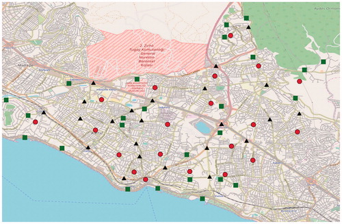
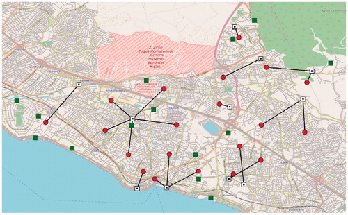
As mentioned before, we also executed the GA on the data of the Kartal district of Istanbul provided by Kılcı et al. (2015). This data set specifies the candidate shelter locations, their capacities, population nodes, locations and their number of inhabitants. It contains 20 PNs that represent 20 sub-districts in Kartal, as well as 25 CLs selected according to various criteria. The PNs are considered as the centers of each sub-district. We illustrate the Kartal district map, PNs and CLs in Figure 1. The PNs are represented by red dots and CLs are represented by green squares. The black triangles indicate the junction points that we selected. We were able to generate a larger number of scenarios (2000), as the GA can handle this problem size.

Figure 1. Kartal district map and the node locations.

To make this data set consistent with our problem, we have to generate scenarios as well as a budget, the establishment and expansion costs, and the service level. We take the service level α equal to 0.95. We consider the case that all establishment costs are the same and equal to 1000. The budget and expansion costs are randomly generated by the same procedure that we used for the benchmark instances in Section 5.2.1.

Before generating the scenarios, first we need to build the road network. In order to do that we identify 23 main road junction points and add them to the node set. Then we calculate the shortest path between each pair of nodes using ArcGIS Pro 2.0.0 with real road network data. We construct a network with 68 nodes and the edges between each pair of them considering the shortest path value as the length of the edge. To have an approximation of the real network, we omit the edges which have length more than 2 km. As a result, our network has 1206 edges and 68 nodes. Scenarios are generated in the same way as we generated scenarios for the benchmark instances using the Network Sampling Algorithm presented in Section 5.2.1. We test six different instances with different number of scenarios: 50, 100, 200, 500, 1000, and 2000. In these six instances the scenario sets are generated independently. For example, the 50 scenarios do not necessarily appear among the 100 scenarios. We present the results for these six problems in Table 5. The column labels are the same as the ones in Tables 3 and 4. We observe that the runtime increases almost linearly with the number of scenarios. We also observe that the best objective value starts to converge as the number of scenarios reaches 2000. Therefore, for the remaining analyses we fixed the number of scenarios to 2000.

Table 5. Results of the Kartal case.

Instance	# PN	# CL	# S	Best obj	Avg. obj	Avg. time
Istanbul_50	20	25	50	1661.54	1662.73	29.16
Istanbul_100	20	25	100	1924.25	1925.01	94.42
Istanbul_200	20	25	200	1365.15	1365.15	122.90
Istanbul_500	20	25	500	1380.99	1380.99	179.90
Istanbul_1000	20	25	1000	1403.97	1403.98	334.34
Istanbul_2000	20	25	2000	1410.87	1410.87	600.05

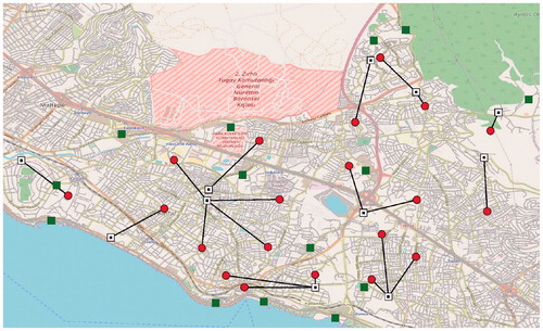
We show the solutions of Istanbul_50 and Istanbul_2000 instances on the Kartal map to see the differences entailed by the number of scenarios. Figures 2 and 3 demonstrate the locations where we decide to open facilities and how we allocate the PNs to those open facilities. Open facilities are identified with white squares and allocations are shown by black lines between PNs and assigned CLs. We see that the open facility locations change significantly between the two solutions.

Figure 2. Solution of Istanbul_50.

5.4. Comparison between ex ante and ex post measures

As explained in Section 3, ex ante and ex post inequity measurements are two different approaches towards inequity quantification under uncertainty. We suggest to use a combination of these two concepts, but it may be instructive to see their differences if applied in pure form. Thus, in this subsection, we compare the solutions found by solving the ex ante and the ex post versions of the problem, defined in Section 3.1, separately from each other. This is achieved by setting the parameter γ in Equation (17)(17) $$\begin{array}{l}\min \gamma \left(\frac{1}{N}\sum _{k\in K}\sum _{s\in S}\sum _{j\in J}{p}_s{b}_k^s{y}_{kj}{d}_{kjs}+\frac{\lambda }{N^2}\sum _{k\in K}\sum _{k\prime \in K}({\tau }_{k,k\prime }^{+}+{\tau }_{k,k\prime }^{-})\right)\\ +(1-\gamma )(\sum _{s\in S}\sum _{k\in K}\sum _{j\in J}\frac{1}{N{\prime }_s}{p}_s{b}_k^s{y}_{kj}{d}_{kjs}+\lambda \sum _{s\in S}{p}_s\frac{1}{N{\prime }_s^2}\sum _{k\in K}\sum _{k\prime \in K}{b}_k^s{b}_{k\prime }^s({\rho }_{kk\prime s}^{+}+{\rho }_{kk\prime s}^{-})),\end{array}$$(17) to the values of one and zero, respectively. We select the instance Istanbul_2000 as our test case. The solutions of the two problem versions are presented in Figures 4 and 5. The solution to the original problem where $\gamma =0.5$ is given in Figure 3.

Figure 3. Solution of Istanbul_2000.

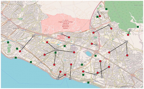
Figure 4 Ex ante problem solution.

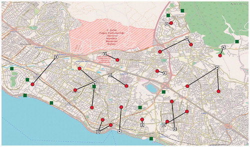
Figure 5. Ex post problem solution.

Table 6 presents the values of the two objective function components to compare the solutions of the ex ante, the ex post, and the combined problem. The second line of Table 6 shows the mean distance measure ADTS, calculated by the combined approach (see end of Section 3). Similarly, the third line shows GMAD, again computed by the combined approach. There is no solution dominating another one. However, it can be observed that eight facility locations are common in the solutions.

Table 6. Evaluation of the solutions of the problem versions.

Problem	Ex ante	Ex post	Combined
ATDS	1135.16	1147.35	1137.61
GMAD	610.24	580.64	599.85

5.5. Tradeoff between efficiency and equity

A major contribution of this work is the introduction of a Gini-related component in the objective function while modeling a stochastic shelter location problem. Therefore, it is worthy to see how this component affects the fairness of the best solution provided by the GA. We first solve the Istanbul_2000 instance without the Gini part in the objective function by setting λ equal to zero, meaning that we neglect equity. Then, we determine the solution obtained for the other extreme case where the objective function is replaced by the GMAD of distances (this corresponds to the limiting case for $\lambda \to \infty$). The two solutions are shown in Figures 6 and 7. We can see that the distances traveled are generally longer but more equitable in Figure 7, compared with Figure 6. It is clear that the solution in Figure 7 pays a too high price for equity. For example, it assigns the upmost PN a more remote shelter than necessary, which is certainly undesirable.

Figure 6. Optimizing the combined ADTS for Istanbul_2000.

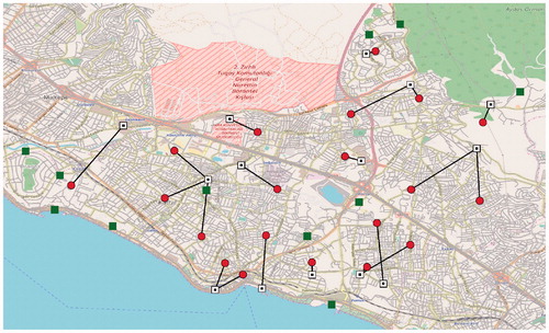
Figure 7. Optimizing the combined GMAD for Istanbul_2000.

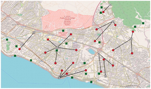
So we are interested in compromise solutions obtained by taking weighted means with varying weights λ. The theory of symmetric comonotonically linear functionals guarantees that the above-mentioned undesirable behavior cannot occur as long as $\lambda \le 0.5$.

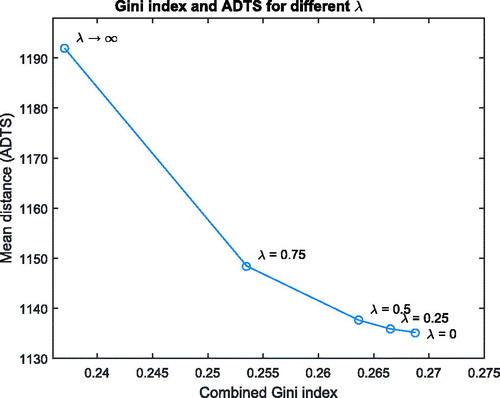
The obtained values for ADTS, for GMAD, and for the Gini index (both in an ex ante and an ex post version) are presented in Table 7 for each of the two extreme problems mentioned above $(\lambda =0$ and $\lambda \to \infty$, respectively), as well as for the compromise approaches where λ is equal to 0.25, 0.5, and 0.75. For the indicated theoretical reasons, λ should be at most 0.5. However, it is interesting also to see how the solution changes when a higher weight is assigned to the equity measure.

Table 7. Evaluation measures for Istanbul_2000 under different values of λ.

Problem	ADTS	GMAD	EAGI	EPGI	MaxED	MinED	RangeED
λ = 0	1135.15	610.24	0.2107	0.2760	2269.23	659.42	1609.81
$\lambda =0.25$	1135.87	605.36	0.2111	0.2734	2312.65	659.42	1653.23
$\lambda =0.5$	1137.61	599.85	0.2106	0.2702	2312.65	755.62	1557.03
$\lambda =0.75$	1148.42	582.28	0.2065	0.2593	2312.65	931.91	1380.74
$\lambda \to \infty$	1191.97	565.06	0.2094	0.2404	2696.41	931.91	1764.50

The first column indicates the weight λ. The second column reports the combined measure for the mean distance that an individual has to traverse in order to reach the assigned shelter (ADTS), cf. end of Section 3. The third column shows GMAD for each problem, again computed by the combined approach. The two next columns, EAGI and EPGI, present the Gini index itself, calculated in a pure ex ante and a pure ex post consideration, respectively. The columns MaxED and MinED indicate the maximum and the minimum expected distance of a population node from the assigned shelter. The last column shows the range of these expected distances, i.e., the difference between MaxED and MinED.

Figure 8 illustrates how the Gini index – we take here the combined version – and the mean distance change with the “weight of equity” λ. It can be seen that by increasing λ from zero to 0.25, the Gini index is decreased, but the mean distance stays at almost the same level. Also, if we further increase λ from 0.25 to 0.5, the mean distance increases only marginally, compared with a much stronger decrease in the Gini index. Therefore, selecting λ equal to 0.5, which is still in line with theoretical recommendations, may be a reasonable choice: it already provides a perceptible reduction of the Gini index (and of the range between maximal and minimal distances) at negligible costs in terms of the average distance. When judging the magnitude of the Gini index reduction, one should be aware that for location decisions, a comparably high “base level” of inequity is unavoidable, since wherever a facility is established, it obviously favors the inhabitants in its immediate neighborhood.

Figure 8. Mean distance and Gini index in dependence of λ for Istanbul_2000.

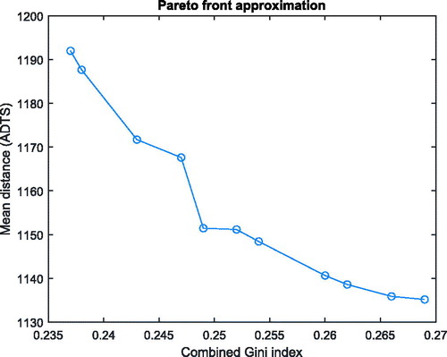
We also carried out a (rough) bi-objective analysis by determining an approximation to the Pareto frontier of the problem with objectives “(expected) combined Gini index” (f_CGI) and “(expected) mean distance” (f_ADTS). At first we minimized each of these two objectives separately. Let us call the minimum value found for mean distance and combined Gini index, $f_{\mathit{\text{ADTS}}}^{min}$ and $f_{CGI}^{min}$, respectively. Then we constructed a new objective by taking a linear combination of normalization of these two objectives: $$f=\omega \times \frac{f_{CGI}}{f_{CGI}^{min}}+(1-\omega )\times \frac{f_{\mathit{\text{ADTS}}}}{f_{\mathit{\text{ADTS}}}^{min}}.$$

In order to explore the full range of the Pareto frontier, the single-objective problems were solved by our GA for the 21 different values $0,0.05,0.10,\dots ,0.95,1$ of the weight ω. The following results refer to the Istanbul$\_2000$ case as described before. Dominated solutions with respect to the two indicated objective functions were removed. Figure 9 shows the Pareto frontier approximation. Note that in the bi-objective analysis, the second term of the weighted sum is the (normalized) Gini index and not GMAD, as in the results on which Figure 8 is based. Obviously, also so-called unsupported solutions (Pareto-optimal solutions that are not optimizers of the single-objective weighted-sum problem for some weight ω) have a nonzero chance of being found in this way, since the GA solves the problem only heuristically.

Figure 9. Approximation of the full range of the Pareto frontier for Istanbul case.

6. Conclusion

In this article we introduced a stochastic shelter location and demand allocation problem for natural disaster preparation that aims to maximize an objective combining efficiency and equity. To the best of our knowledge, this is the first that includes a measure derived from the Gini index within a stochastic optimization framework to account for fairness. We represented uncertainty in demand and transportation network damage by means of a set of scenarios and suggested to obtain the scenarios by generating the network damage randomly with respect to link-level correlation. We considered uncertainty in the objective by a combination of ex ante and ex post inequity concepts from the literature on decision theory.

First we formulated the problem as a MIP model and showed that it cannot be solved efficiently by a commercial MIP solver on benchmark instances. We tested problem with sizes that would arise in real applications. We next developed a GA for our problem and introduced specialized enhancements in the algorithm by utilizing a relaxed allocation model in order to improve the performance. We used the benchmark instances to compare the exact solutions with the GA solutions. Our results showed that the GA outperforms Cplex in terms of runtime in almost all instances. Furthermore, the GA obtains either the optimal solutions or solutions that are very close to optimal ones, with 0.42 percentage optimality gap on the average over different problem sizes.

We also executed the GA on real data from the Kartal district of Istanbul provided by Kılcı et al., (2015) expanded with additional parameters. The GA solved this instance with 20 PNs, 25 CLs, and 2000 scenarios in around 10 minutes in our computational platform. We analyzed the tradeoff between efficiency (mean distance) and equity (GMAD of distances), and we also compared the solutions obtained from pure ex ante and ex post approaches.

A future research direction concerns the replacement of the allocation subproblem with a representation of the behavior of disaster victims when seeking for shelter. In addition, different alternative approaches for incorporating inequity aversion into optimization might also deserve investigation. Moreover, our model assumes a risk-neutral decision maker. An interesting topic of future research is the inclusion of measures for risk averseness, which is especially appropriate for disaster relief applications. A suitable way to do that would be to add penalties for the CVaR, or to impose constraints on the CVaR. For an example of the application of CVaR penalties or CVaR constraints in humanitarian logistics, we refer the reader to Elçi and Noyan (2018) and Noyan et al. (2017), respectively. We carried out preliminary experiments using CVaR constraints on total excess demand on the one hand and total capacity expansion on the other hand. Although in these experiments, the additional constraints did not change the properties of the solutions to a large extent, the topic deserves a more comprehensive investigation in the future. In particular, efficient algorithms (both exact and heuristic) should be developed for this extension.

Additional information

Notes on contributors

Mahdi Mostajabdaveh

Mahdi Mostajabdaveh is a Ph.D. candidate in the Industrial Engineering Department of the College of Engineering at Koç University in Istanbul, Turkey. His M.Sc. and B.Sc. degrees are in industrial engineering from Sharif University of Technology, Tehran, Iran. His research interests include humanitarian logistic, facility location, vehicle routing and metaheuristic algorithms.

Walter J. Gutjahr

Walter J. Gutjahr received his doctoral degree in mathematics from the University of Vienna. After a career in industrial software engineering management at Siemens Corporation, he returned to the University of Vienna, where he held positions as an associate professor and later as a full professor of applied mathematics and computer science. His current research interests include multi-criteria decision analysis, stochastic optimization, project scheduling, healthcare management, and humanitarian logistics. He has published more than 110 peer-reviewed articles, most of them in high-level international journals, and has been invited keynote speaker of several international conferences. He serves as a co-editor of OR Spectrum, as an associate editor of Central European Journal of Operations Research, and as a member of the editorial boards of several other journals.

F. Sibel Salman

F. Sibel Salman is an associate professor at the Industrial Engineering Department of the College of Engineering at Koç University in Istanbul, Turkey. Prior to joining Koç University, she held a faculty position at the Krannert School of Management, Purdue University, USA. She got her Ph.D. in operations research from Carnegie Mellon University, USA, and her M.Sc. and B.Sc. degrees from Bilkent University, Turkey. She has published over 30 articles in various international journals in the areas of disaster logistics, supply chain management, retail operations management, telecommunication network design, production scheduling, design of approximation algorithms and combinatorial optimization. She has been/is in the editorial board of the journals Computers and Operations Research, and Production and Operations Management.

References

- Afshar A. and Haghani, A. (2012) Modeling integrated supply chain logistics in real-time large-scale disaster relief operations. Socio-Economic Planning Sciences, 46(4), 327–338.
- Alp, O., Erkut, E. and Drezner, Z. (2003) An efficient genetic algorithm for the p-median problem. Annals of Operations Research, 122(1), 21–42.
- Balcik, B., Iravani, S.M. and Smilowitz, K. (2010) A review of equity in nonprofit and public sector: A vehicle routing perspective, in Wiley Encyclopedia of Operations Research and Management Science, Wiley, Hoboken, NJ.
- Bayram. V. (2016) Optimization models for large scale network evacuation planning and management: A literature review. Surveys in Operations Research and Management Science, 21(2), 63–84.
- Bayram, V., Tansel, B.C. and Yaman. H. (2015) Compromising system and user interests in shelter location and evacuation planning. Transportation Research Part B: Methodological, 72, 146–163.
- Bayram V. and Yaman, H. (2017) Shelter location and evacuation route assignment under uncertainty: A Benders decomposition approach. Transportation Science, 52(2), 416–436.
- Beasley. J.E. (1988) An algorithm for solving large capacitated warehouse location problems. European Journal of Operational Research, 33(3), 314–325.
- Ben-Porath, E., Gilboa, I. and Schmeidler, D. (1997) On the measurement of inequality under uncertainty. Journal of Economic Theory, 75(1), 194–204.
- Boonmee, C., Arimura, M. and Asada, T. (2017) Facility location optimization model for emergency humanitarian logistics. International Journal of Disaster Risk Reduction, 24(Supplement C), 485–498.
- Bozorgi-Amiri, A., Jabalameli, M. and Al-e Hashem, S.M. (2013) A multi-objective robust stochastic programming model for disaster relief logistics under uncertainty. OR Spectrum, 35(4), 905–933.
- Chew S.H. and Sagi, J.S. (2012) An inequality measure for stochastic allocations. Journal of Economic Theory, 147(4), 1517–1544.
- Coutinho-Rodrigues, J., Tralho, L. and Alada-Almeida, L. (2012) Solving a location-routing problem with a multiobjective approach: The design of urban evacuation plans. Journal of Transport Geography, 22, 206–218.
- Derbel, H., Jarboui, B., Hanafi, S. and Chabchoub, H. (2012) Genetic algorithm with iterated local search for solving a location-routing problem. Expert Systems with Applications, 39(3), 2865–2871.
- Döyen, A., Aras, N. and Barbarosoğlu, G. (2012) A two-echelon stochastic facility location model for humanitarian relief logistics. Optimization Letters, 6(6), 1123–1145.
- Drezner, T., Drezner, Z. and Guyse, J. (2009) Equitable service by a facility: Minimizing the Gini coefficient. Computers & Operations Research, 36(12), 3240–3246.
- Eiben, A.E. and Smith, J.E. (2003) Introduction to Evolutionary Computing, Springer, Berlin.
- Eisenhandler, O. and Tzur, M. (2016) The humanitarian pickup and distribution problem.
- Elçi Ö. and Noyan, N. (2018) A chance-constrained two-stage stochastic programming model for humanitarian relief network design. Transportation Research Part B: Methodological, 108, 55–83.
- Fleurbaey, M., Gajdos, T. and Zuber, S. (2015) Social rationality, separability, and equity under uncertainty. Mathematical Social Sciences, 73, 13–22.
- Gajdos, T. and Maurin, E. (2004) Unequal uncertainties and uncertain inequalities: An axiomatic approach. Journal of Economic Theory, 116(1), 93–118.
- Galindo G. and Batta, R. (2013) Prepositioning of supplies in preparation for a hurricane under potential destruction of prepositioned supplies. Socio-Economic Planning Sciences, 47(1), 20–37.
- Gopalan, R., Kolluri, K.S., Batta, R. and Karwan, M.H. (1990) Modeling equity of risk in the transportation of hazardous materials. Operations Research, 38(6), 961–973.
- Gralla, E., Goentzel, J. and Fine, C. (2014) Assessing trade-offs among multiple objectives for humanitarian aid delivery using expert preferences. Production and Operations Management, 23(6), 978–989.
- Grass, E. and Fischer, K. (2016) Two-stage stochastic programming in disaster management: A literature survey. Surveys in Operations Research and Management Science, 21(2), 85–100.
- Gutjahr, W.J. and Dzubur, N. (2016) Bi-objective bilevel optimization of distribution center locations considering user equilibria. Transportation Research Part E: Logistics and Transportation Review, 85, 1–22.
- Gutjahr, W.J. and Fischer, S. (2018) Equity and deprivation costs in humanitarian logistics. European Journal of Operational Research, 270(1), 185–197
- Gutjahr, W.J. and Nolz, P.C. (2016) Multicriteria optimization in humanitarian aid. European Journal of Operational Research, 252(2), 351–366.
- Holguín-Veras, J., Pérez, N., Jaller, M., van Wassenhove, L.N. and Aros-Vera, F. (2013) On the appropriate objective function for post-disaster humanitarian logistics models. Journal of Operations Management, 31(5), 262–280.
- Holland, J.H. (1992) Genetic algorithms. Scientific American, 267(1), 66–73.
- Hoyos, M.C., Morales, R.S. and Akhavan-Tabatabaei, R. (2015) OR models with stochastic components in disaster operations management: A literature survey. Computers & Industrial Engineering, 82 (Supplement C), 183–197.
- Hu, S.-L., Han, C.-F. and Meng, L.-P. (2016) Stochastic optimization for investment in facilities in emergency prevention. Transportation Research Part E: Logistics and Transportation Review, 89, 14–31.
- Huang, M., Smilowitz, K. and Balcik, B. (2012) Models for relief routing: Equity, efficiency and efficacy. Transportation Research Part E: Logistics and Transportation Review, 48(1), 2–18.
- Jaramillo, J.H., Bhadury, J. and Batta, R. (2002) On the use of genetic algorithms to solve location problems. Computers & Operations Research, 29(6), 761–779.
- Karsu, Ö. and Morton, A. (2015) Inequity averse optimization in operational research. European Journal of Operational Research, 245(2), 343–359.
- Kılcı, F., Kara, B.Y. and Bozkaya, B. (2015) Locating temporary shelter areas after an earthquake: A case for Turkey. European Journal of Operational Research, 243(1), 323–332.
- Kongsomsaksakul, S., Yang, C. and Chen, A. (2005) Shelter location-allocation model for flood evacuation planning. Journal of the Eastern Asia Society for Transportation Studies, 6, 4237–4252.
- Kulshrestha, A., Wu, D., Lou, Y. and Yin, Y. (2011) Robust shelter locations for evacuation planning with demand uncertainty. Journal of Transportation Safety & Security, 3(4), 272–288.
- Li, L., Jin, M. and Zhang, L. (2011) Sheltering network planning and management with a case in the gulf coast region. International Journal of Production Economics, 131(2), 431–440.
- Lin, Y.-H., Batta, R., Rogerson, P.A., Blatt, A. and Flanigan, M. (2011) A logistics model for emergency supply of critical items in the aftermath of a disaster. Socio-Economic Planning Sciences, 45(4), 132–145.
- Marsh, M.T. and Schilling, D.A. (1994) Equity measurement in facility location analysis: A review and framework. European Journal of Operational Research, 74(1), 1–17.
- Ng, M., Park, J. and Waller, S.T. (2010) A hybrid bilevel model for the optimal shelter assignment in emergency evacuations. Computer-Aided Civil and Infrastructure Engineering, 25(8), 547–556.
- Noyan, N. (2012) Risk-averse two-stage stochastic programming with an application to disaster management. Computers & Operations Research, 39(3), 541–559.
- Noyan, N., Balcik, B. and Atakan, S. (2015) A stochastic optimization model for designing last mile relief networks. Transportation Science, 50(3), 1092–1113.
- Noyan, N., Merakli, M. and Kucukyavuz, S. (2017) Two-stage stochastic programming under multivariate risk constraints with an application to humanitarian relief network design. arXiv preprint: arXiv:1701.06096.
- Ogryczak, W. (2000) Inequality measures and equitable approaches to location problems. European Journal of Operational Research, 122(2), 374–391.
- Ortuño, M., Tirado, G. and Vitoriano, B. (2011) A lexicographical goal programming based decision support system for logistics of humanitarian aid. Top, 19(2), 464–479.
- Paul, J.A. and MacDonald, L. (2016) Location and capacity allocations decisions to mitigate the impacts of unexpected disasters. European Journal of Operational Research, 251(1), 252–263.
- Ransikarbum, K. and Mason, S.J. (2016) Goal programming-based post-disaster decision making for integrated relief distribution and early-stage network restoration. International Journal of Production Economics, 182, 324–341.
- Rath, S., Gendreau, M. and Gutjahr, W.J. (2015) Bi-objective stochastic programming models for determining depot locations in disaster relief operations. International Transactions in Operational Research, 23(6), 997–1023, 2015.
- Rawls, C.G. and Turnquist, M.A. (2010) Pre-positioning of emergency supplies for disaster response. Transportation Research Part B: Methodological, 44(4), 521–534.
- Renkli, Ç. and Duran, S. (2015) Pre-positioning disaster response facilities and relief items. Human and Ecological Risk Assessment: An International Journal, 21(5), 1169–1185.
- Rezaei-Malek, M. and Tavakkoli-Moghaddam, R. (2014) Robust humanitarian relief logistics network planning. Uncertain Supply Chain Management, 2(2), 73–96.
- Romeijn, H.E. and Morales, D.R. (2000) A class of greedy algorithms for the generalized assignment problem. Discrete Applied Mathematics, 103(1), 209–235.
- Salman, F.S. and Yücel, E. (2015) Emergency facility location under random network damage: Insights from the Istanbul case. Computers & Operations Research, 62, 266–281.
- Tricoire, F., Graf, A. and Gutjahr, W.J. (2012) The bi-objective stochastic covering tour problem. Computers & Operations Research, 39(7), 1582–1592
- Trivedi, A. and Singh, A. (2017) A hybrid multi-objective decision model for emergency shelter location-relocation projects using fuzzy analytic hierarchy process and goal programming approach. International Journal of Project Management, 35(5), 827–840.
- Tzeng, G.-H., Cheng, H.-J. and Huang, T.D. (2007) Multi-objective optimal planning for designing relief delivery systems. Transportation Research Part E: Logistics and Transportation Review, 43(6), 673–686.
- Ukkusuri, S. and Yushimito, W. (2008) Location routing approach for the humanitarian prepositioning problem. Transportation Research Record: Journal of the Transportation Research Board, 2089, 18–25.
- Uster, H. and Dalal, J. (2107) Strategic emergency preparedness network design integrating supply and demand sides in a multi-objective approach. IISE Transactions, 49(4), 395–413.
- Verma, A. and Gaukler, G.M. (2015) Pre-positioning disaster response facilities at safe locations: An evaluation of deterministic and stochastic modeling approaches. Computers & Operations Research, 62, 197–209.
- Vitoriano, B., Ortuno, M.T., Tirado, G. and Montero, J. (2011) A multi-criteria optimization model for humanitarian aid distribution. Journal of Global Optimization, 51(2), 189–208.
- Wang, W., Yang, S., Hu, F., He, S., Shi, X., Meng, Y. and Shi, M. (2016) Integrated optimization model for shelter allocation and evacuation routing with consideration of reliability. Transportation Research Record: Journal of the Transportation Research Board, 2599, 33–42.
- Yitzhaki, S. and Schechtman, E. (2013) More than a dozen alternative ways of spelling Gini, in The Gini Methodology, pp. 11–31, Springer, New York, NY.
- Yücel, E., Salman, F.S. and Arsik, I. (2018) Improving post-disaster road network accessibility by strengthening links against failures. European Journal of Operational Research, 269(2), 406–422.