Machine tools with hidden defects: Optimal usage for maximum lifetime value

Abstract

We consider randomly failing high-precision machine tools in a discrete manufacturing setting. Before a tool fails, it goes through a defective phase where it can continue processing new products. However, the products processed by a defective tool do not necessarily generate the same reward obtained from the ones processed by a normal tool. The defective phase of the tool is not visible and can only be detected by a costly inspection. The tool can be retired from production to avoid a tool failure and save its salvage value; however, doing so too early causes not fully using the production potential of the tool. We build a Markov decision model and study when it is the right moment to inspect or retire a tool with the objective of maximizing the total expected reward obtained from an individual tool. The structure of the optimal policy is characterized. The implementation of our model by using the real-world maintenance logs at the Philips shaver factory shows that the value of the optimal policy can be substantial compared to the policy currently used in practice.

Key Words:

• Markov decision processes
• manufacturing operations
• inspection planning
• tool management

1. Introduction

High-precision machining refers to cutting metal or other rigid materials with tolerances in the single-digit micron range; it is used in many areas with stringent quality requirements such as aerospace, electronics, defense, and medical technology (Groover, 2016). Although high-precision machine tools can be very expensive, many manufacturers under-utilize them, as they lack a scientific approach to optimization (Probst, 2015). An important challenge in the industry is to be able to use these tools effectively and obtain the maximum value out of them.

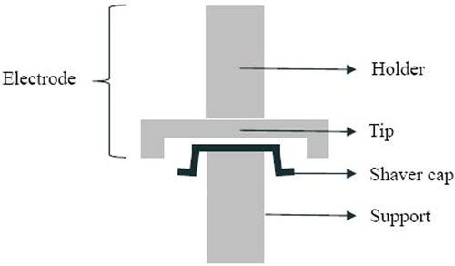
In this article, we consider maximizing the value of high-precision machining tools by optimizing their inspection and retirement decisions. The motivation comes from our collaboration with Philips Consumer Lifestyle, a global consumer-electronics manufacturer. The company produces electric shavers by using highly precise Electro-Chemical Machining (ECM) tools. These tools are responsible for cutting small openings in the round caps covering the blades of electric shavers (see Figure 6). After processing a random amount of products, the tool fails. This means the tool becomes unusable and is discarded. If a tool is retired before its failure, then the tool can be salvaged to generate an additional reward. That is, retiring a tool prior to its failure saves the tool’s salvage value, however, doing it too early means that its production capacity is not fully used. Furthermore, before the tool fails, it first goes into a hidden defective phase, which can only be detected with the inspection of the tool. A defective tool can also lead to products that are less valuable than the ones processed with a healthy tool. Hence, the company faces the problem of finding the optimal tool usage policy, which specifies when to execute an inspection based on the number of products produced since the tool’s last inspection and during its entire lifetime. This problem is relevant for many other applications where capital assets generate a reward at every unit of usage under the risk of a costly failure and require inspections to reveal their true conditions.

In the case of Philips, the acquisition of the tools is made at a strategic level considering factors such as growth scenarios and available budget. Since such strategic decisions are already made, the production department follows the operational objective of maximizing the economic value of an individual tool to achieve a high return on investment. This is also often seen for cutting tools in a flexible manufacturing system. We therefore focus on the total expected reward a tool collects over its lifetime, which we refer to as the tool’s lifetime value. The tool usage policy at Philips is based on two product counters: run counter and cumulative counter. The run counter is the number of products processed by the tool since its last inspection, whereas the cumulative counter is the total number of products processed by the tool. The tool is inspected every time its run counter hits a fixed inspection limit and retired as soon as it is found to be defective. We refer to this strategy as the fixed-threshold policy. The first limitation of this policy is to have a fixed inspection limit regardless of the age of the tool. Second, it is unable to capture the trade-off between the risk of a tool failure and fully exploiting the production potential of the tool.

We answer the following research questions:

1. What is the optimal tool usage policy that maximizes the lifetime value of a tool?

2. To facilitate the implementation of the optimal policy in practice, can we characterize the structure of the optimal policy in terms of product counters?

3. How much does a tool’s lifetime value increase under the optimal policy compared with the fixed-threshold policy? What is the value of postponing the retirement of a defective tool?

4. How to solve for the optimal policy efficiently for industry-size problems with large state spaces?

To find the optimal tool-usage policy, we formulate a stochastic shortest path problem, which is a class of total-cost Markov decision models with a cost-free absorbing termination state (Bertsekas and Tsitsiklis, 1991). The resulting optimal policy is practically attractive as it is specified in terms of easy-to-track product counters. Assuming that the amount of products the tool can process in the normal and defective phases have general probability distributions, we provide a structural analysis of the optimal tool-usage policy. The implementation of our model with parameters estimated from a case study at Philips shows that, depending on the cost parameters, the percentage improvement over the optimal fixed-threshold policy can take values from 5.2% to 20.7%.

The remainder of this article is organized as follows. Section 2 surveys the relevant literature. Section 3 presents the model formulation and Section 4 establishes the structural results on the optimal policy. Section 5 discusses the numerical insights and Section 6 presents a case study based on the real-world maintenance logs at Philips. Section 7 concludes this article with future research directions. An electronic companion includes the proofs and supplementary results.

2. Literature

This article is related to research on maintenance optimization on systems with the following characteristics:

1. Three-state degradation process with hidden healthy and defective states and a self-announcing failed state (i.e., the delay-time model) under generally distributed sojourn times for healthy and defective states.

2. Total expected cost over the lifetime of an asset is the performance criterion.

3. Degradation process is governed by a Markov chain with hidden states.

There is a rich literature on delay-time models (Christer, 1982) within the context of inspection planning; see Wang (2012) for a review of delay-time-based maintenance models. A more recent review can be found in Section 3.2 of de Jonge and Scarf (2019). Most studies in this literature use numerical analysis based on renewal theory with the objective of minimizing average cost (or maximizing average reward) on an infinite horizon (e.g., Christer and Wang, 1995; Wang and Christer, 2003, Scarf et al., 2009; Jiang, 2017; Arts and Basten, 2018; Duan et al., 2019). Maillart and Pollock (2002) consider generally distributed sojourn times for the normal and defective phases and build an infinite-horizon average-cost Markov decision model to compute the optimal inspection schedule. MacPherson and Glazebrook (2011) extend Maillart and Pollock (2002) by adding a repair option to fix a defective component, and propose a heuristic solution based on policy improvement. None of these studies allows postponing the renewal of a defective system.

There is a recent interest in postponing the replacement of a defective component under the delay-time model. Van Oosterom et al. (2014) consider periodic inspections and allow for postponed replacement after an inspection. However, they do this under the assumptions of an exponentially-distributed time to a defect, and a deterministic duration for the defective state. Under generally distributed sojourn times, Yang et al. (2016) consider both periodic and random inspections and allow for postponed replacement after a random inspection. Berrade et al. (2017) also allow postponed replacement after a periodic inspection. Yang et al. (2019) introduce a two-phase maintenance policy, where the first phase includes inspections and the second phase includes the preventive replacement, potentially postponing the replacement of a defective component. However, none of these studies allow incurring a cost due to working in the defective condition. In our work, we allow postponement and incur a cost use to working in the defective condition. To the best of our knowledge, the structure of the optimal policy has not been studied before under the possibility of working with a defective system in the presence of general distributions for the duration of normal and defective states. We do this under an objective function that considers the finite lifetime of an individual production asset.

The majority of the maintenance optimization literature considers infinite-horizon objectives (Khojandi et al., 2014). However, this does not apply to the problem faced by the operators of expensive machining tools described in Section 1. In accordance with the practical desire to maximize the return-on-investment from an individual tool, we consider the total expected reward that can be obtained from a tool as the objective. The origin of using total expected reward (or cost) in maintenance optimization goes back to Barlow et al. (1963) with a two-state degradation model including a functioning state and a silent failure state. Barlow et al. (1963) minimize the total expected cost over the lifetime of a system by capturing the trade-off between the cost of too frequent inspections and the cost of working with a defective system. The decision problem terminates upon the detection of failure. Barlow et al. (1963) has been extended in several ways. Kaio and Osaki (1984) propose an approximation of the total expected cost to simplify the computation of the inspection schedule. Parmigiani (1996) considers imperfect tests that can be performed before an inspection. Leung (2001) considers the uncertainty in the time-to-failure distribution and obtains minimax inspection schedules. Sengupta (1980) extends Barlow et al. (1963) to a three-state degradation model including a functioning state, a hidden defective phase and a self-announcing failure state. The current article has the same degradation model, however, we have a three-action model (i.e., process, inspect, retire) whereas all the papers above only provide an inspection schedule.

Our work can be seen to relate to maintenance models in which the degradation process is governed by a Markov chain with hidden states. Among the papers with self-announcing failures, Ozekici and Pliska (1991) study a system similar to ours, but assume that the duration of the defective state is exponentially distributed and preventive maintenance decisions follow a predetermined stopping rule. Ohnishi et al. (1986) express the deterioration process as a continuous-time Markov chain and show the optimal time interval between successive inspections decreases as the degree of deterioration increases. Makis and Jiang (2003) model the evolution of the machine state as a continuous-time Markov process together with a discrete-time observation process depending on the hidden machine state. The optimal replacement policy is found by minimizing the average cost-rate in the long-run by using optimal stopping theory. Maillart (2006) and Kim and Makis (2013) model the deterioration process with self-announcing failures as discrete-time and continuous-time Markov chains, respectively, with the objective of minimizing the average cost rate over an infinite horizon. These two papers are similar in showing that the at-most-four-region policy is optimal and derive structural properties of the optimal policy. Maillart (2006) does not consider the cost of operating under a deteriorated system, and Kim and Makis (2013) assume that the system is replaced immediately when it is found in the defective state. In the current article, we do not have these limitations. More recently, Moghaddass and Ertekin (2018) consider a hidden semi-Markov degradation process with discrete-time condition monitoring and study the joint ordering and replacement. A common approach in this stream is to use a partially observable Markov decision process model with a belief state, representing a probability distribution over the hidden states. In our problem, the defective state of the tool is hidden, but the degradation states do not evolve according to a Markov chain. Instead, we derive the history-dependent transition probabilities of our Markov decision process from the probability distributions in the delay-time model. This modeling approach is also practically appealing, as the optimal policy becomes a function of easy-to-track variables instead of a belief state. It further helps us in avoiding the computational burden to solve for the optimal policy in the presence of an uncountable set of belief states.

3. Model

3.1. Tool degradation process

We consider a tool that first goes into a defective phase before it fails. The tool failure immediately announces itself, whereas the defective phase is not visible and only an inspection can detect it. Let X denote the random variable that represents the product number at which the tool becomes defective (e.g., X = 5 means that the tool processed four products in the normal phase and the fifth product in the defective phase). The sample space of X is $\{1,2,\dots ,n_X\}$ with $n_X\in \mathbb{N}.$ We let H denote the number of products the tool processes in the defective phase, and it has the sample space $\{0,1,\dots ,n_H\}$ with $n_H\in \left\{0\right\}\cup \mathbb{N}.$ Notice that n_H can be equal to zero, meaning that a defect can immediately cause a self-announcing failure. Also, note that n_X and n_H can take any large value, and therefore, do not put a limitation to our model.

The probability mass function (pmf) and cumulative distribution function (cdf) of X are denoted with $f_X(·)$ and $F_X(·),$ respectively. Likewise, the pmf and cdf of H are denoted with $f_H(·)$ and $F_H(·).$ We let ${\overline{F}}_X(x)={\sum }_{i=x}^{n_X}{f}_X(i)$ and ${\overline{F}}_H(h)={\sum }_{i=h}^{n_H}{f}_H(i).$ For notational convenience in our analysis, we extend the support of the random variable X and define $f_X(x)=0$ and ${\overline{F}}_X(x)=0$ for all $x>n_X.$ Similarly, we define $f_H(h)=0$ and ${\overline{F}}_H(h)=0$ for all $h>n_H.$

3.2. Problem description

The decision epochs correspond to the moments the tool is ready to process a new product (i.e., after the tool is first installed, after the processing of one product, or after an inspection). One of the following actions is taken in each decision epoch: process the next product (P), inspect the tool (I), and retire the tool (R). Inspection is permitted only if the degradation phase of the tool is not known with certainty. An inspection resets the run counter to zero and correctly reveals the true degradation phase of the tool at cost $C_i>0.$ The inspection cost C_i captures the cost of examining the tool with skilled technicians as well as the costs of removing the tool for inspection, its re-installation and follow-up calibration. If the tool is retired before being damaged with a failure, then the tool can be salvaged at a higher value. We let $C_r\ge 0$ denote the salvage reward that captures the economic gain obtained by retiring the tool before it fails. The lifetime of the tool ends with the failure, and a failed tool does not bring any salvage reward. The cost of inconvenience due to a failed tool is negligible (i.e., such a cost could still be modeled by adjusting C_r accordingly). If a product is processed with no tool failure, both the cumulative counter and run counter increase by one unit. Processing a product with a healthy tool brings a reward m > 0 per product. If the tool is defective, it brings a reward $m-C_d$ per product, where C_d captures the economic loss associated with processing a product with a defective tool (e.g., cost of lower quality, cost of rework, etc.). It is assumed that $0\le C_d<m+C_r.$ The objective is to maximize the expected total reward obtained from an individual tool.

3.3. Markov decision process model

State space. Let v and τ denote the values of the cumulative counter and run counter, respectively, and let u denote the last observed degradation phase of the tool; i.e., $u\in \{0,1\}$ where zero is the normal phase and one is the defective phase. We use the symbol $\nabla$ to represent the end-of-life state of the tool, meaning that the tool is either failed or retired.

Case u = 0: The tool is last observed in the normal phase

The set of states when u = 0 is given by (1) $${\mathcal{S}}_0\triangleq \{(v,\tau ,0):v\in \{0,\dots ,n_X+n_H-1\},\tau \in \{\max (v-n_X+1,0),\dots ,v\left\}\right\}.$$(1)

Notice in Equation (1)(1) $${\mathcal{S}}_0\triangleq \{(v,\tau ,0):v\in \{0,\dots ,n_X+n_H-1\},\tau \in \{\max (v-n_X+1,0),\dots ,v\left\}\right\}.$$(1) that the cumulative counter v can be as low as zero (i.e., a new tool) and it can be at most $n_X+n_H-1,$ as having it equal to $n_X+n_H$ would imply the tool has failed, which is already captured by the state $\nabla .$ Also, if the cumulative counter v reaches n_X, the tool is guaranteed to be in the defective phase. Since inspection is a superfluous action then, the run counter τ must be at least $v-n_X+1$ for $v\ge n_X,$ and therefore, the run counter τ takes values starting from $\max (v-n_X+1,0)$ in Equation (1)(1) $${\mathcal{S}}_0\triangleq \{(v,\tau ,0):v\in \{0,\dots ,n_X+n_H-1\},\tau \in \{\max (v-n_X+1,0),\dots ,v\left\}\right\}.$$(1) . 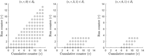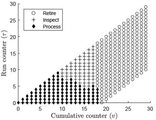Figure 1 (left) illustrates the state space ${\mathcal{S}}_0$ for n_X = 10 and n_H = 4.

Figure 1. State space of the Markov decision process model illustrated for n_X = 10 and n_H = 4.

Case u = 1: The tool is last observed in the defective phase

It is important to note that the set of variables $(v,\tau ,u)$ is not sufficient to capture the production and inspection history of a tool for u = 1, as illustrated in the example below.

Example 1. Suppose that $(v,\tau ,u)=(9,0,1)$ and this state is reached via an inspection at state $(v,\tau ,u)=(9,8,0).$ Then, it can be inferred that $2\le X\le 9.$ However, if the state $(v,\tau ,u)=(9,0,1)$ had been reached via an inspection at state $(v,\tau ,u)=(9,2,0),$ then it could be inferred that $8\le X\le 9.$ That is, the amount of information on X (specifically, the lower bound on the realization of X) is different at state $(v,\tau ,u)=(9,0,1)$ depending on how it is reached.

To capture all the available information in the tool’s history, we introduce an additional state variable w, which we refer to as the inferred lower bound on X. More specifically, if an inspection at cumulative counters v and run counter τ finds the tool in the defective phase, it is possible to infer that $X\ge w$ where $w=v-\tau +1.$ Consequently, the set of states when the tool is last observed in the defective phase (u = 1) is given by (2) $$\begin{array}{c}{\mathcal{S}}_1\triangleq \{(v,\tau ,w,1):v\in \{1,\dots ,n_X+n_H-2\},\\ \tau \in \{\max (v-n_X+1,0),\dots ,\min (v,n_H)-1\},w\in \{1,\dots ,v-\tau \}\}.\end{array}$$(2)

The cumulative counter v starts from one because u = 1 is only possible after an inspection, and v must be at least one for an inspection to be permitted. Also, v can be at most $n_X+n_H-2.$ This is because an inspection could take place latest at cumulative counter $n_X-1,$ and the tool could process at most $n_H-1$ more products before transiting to $\nabla .$ Regarding the possible values of the run counter τ in Equation (2)(2) $$\begin{array}{c}{\mathcal{S}}_1\triangleq \{(v,\tau ,w,1):v\in \{1,\dots ,n_X+n_H-2\},\\ \tau \in \{\max (v-n_X+1,0),\dots ,\min (v,n_H)-1\},w\in \{1,\dots ,v-\tau \}\}.\end{array}$$(2) , we first note that τ must be strictly less than v because $\tau =v$ would mean the tool has never been inspected (which is not possible for u = 1). Also, τ can be at most $n_H-1$ because the tool could process at most $n_H-1$ more products (after identifying the tool as defective in an inspection) before transiting to $\nabla .$ Thus, the run counter τ is at most $\min (v,n_H)-1.$ Finally, we note in Equation (2)(2) $$\begin{array}{c}{\mathcal{S}}_1\triangleq \{(v,\tau ,w,1):v\in \{1,\dots ,n_X+n_H-2\},\\ \tau \in \{\max (v-n_X+1,0),\dots ,\min (v,n_H)-1\},w\in \{1,\dots ,v-\tau \}\}.\end{array}$$(2) that the state variable w never exceeds $v-\tau .$ This is because, when an inspection is performed at cumulative counter v and the tool is found defective, the maximum value of w is the cumulative counter value v itself (when the inspection is performed at run counter 1), and the value of w remains equal to the difference between the cumulative and run counters as the tool continues production in the defective phase. This is illustrated in an example below.

Example 2. Suppose that $(v,\tau ,u)=(9,1,0)$ and an inspection reveals that the tool is defective. Then, it is inferred that X = 9, and therefore, w is updated as the value of v (i.e., w = 9). This is the maximum value of w possible when an inspection is performed at v = 9 and the tool is found defective. Upon finding the tool defective, the state moves from ${\mathcal{S}}_0$ to ${\mathcal{S}}_1$ and it becomes $(v,\tau ,w,u)=(9,0,9,1).$ Subsequently, the state transits to $(v,\tau ,w,u)=(9+i,i,9,1)$ after processing i more products in the defective state, where w remains equal to $v-\tau .$ That is, for u = 1, at any particular value of v and τ, w can be at most $v-\tau .$

Actions, state transitions and rewards. We let $\mu (·)$ denote a function that maps a state into an action. In particular, $\mu (\mathbf{s})\in \{P,I,R\}$ for $\mathbf{s}\in \{(v,\tau ,0)\in {\mathcal{S}}_0:v<n_X,0<\tau \}.$ Since inspection is not permitted if the degradation phase of the tool is known with certainty, it follows that $\mu (\mathbf{s})\in \{P,R\}$ for $\mathbf{s}\in {\mathcal{S}}_1\cup \{(v,\tau ,0)\in {\mathcal{S}}_0:v\ge n_X \mathrm{or} \tau =0\}.$ Let s_k denote the state of the Markov Decision Process (MDP) at the kth decision epoch, $k\in \{0,1,\dots \}.$ In Table 1, we present the state transitions under each possible action with corresponding probabilities and rewards, and further explain them below.

Table 1. Summary of the state transitions with associated probabilities and rewards.

sk	$\mu ({\mathbf{s}}_k)$	${\mathbf{s}}_{k+1}$	$\mathbb{P}({\mathbf{s}}_{k+1}|{\mathbf{s}}_k,\mu ({\mathbf{s}}_k))$	Reward
$(v,\tau ,0)$	I	$(v,0,v-\tau +1,1)$	${\pi }_d(v,\tau )$	$-C_i$
		$(v,0,0)$	$1-{\pi }_d(v,\tau )$	$-C_i$
$(v,\tau ,0)$	P	$(v+1,\tau +1,0)$	$1-{\pi }_{f,0}(v,\tau )$	$m-C_d {\pi }_d(v+1,\tau +1)$
		$\nabla$	${\pi }_{f,0}(v,\tau )$	0
$(v,\tau ,w,1)$	P	$(v+1,\tau +1,w,1)$	$1-{\pi }_{f,1}(v,\tau ,w)$	$m-C_d$
		$\nabla$	${\pi }_{f,1}(v,\tau ,w)$	0
$(v,\tau ,0)$	R	$\nabla$	1	Cr
$(v,\tau ,w,1)$

Suppose that an inspection is done at state $(v,\tau ,0).$ If the tool is found defective, which occurs with the conditional probability: $${\pi }_d(v,\tau )\triangleq \mathbb{P}(X\le v|X>v-\tau ,X+H>v),$$ the state is updated as $(v,0,v-\tau +1,1),$ i.e., this was also seen in Example 2. Otherwise, the state is updated as $(v,0,0).$ Our model allows that the inspection can be immediately followed by the retire-the-tool action if desired.

If the process action is taken at state $(v,\tau ,0),$ the tool fails with the conditional probability: $${\pi }_{f,0}(v,\tau )\triangleq \mathbb{P}(X+H=v+1|X>v-\tau ,X+H>v),$$ and the end-of-life state $\nabla$ is reached. If no failure occurs, the state moves to $(v+1,\tau +1,0)$ and two scenarios are possible: If the tool is still in the normal phase at the completion of the $(v+1)$th product, which occurs with probability: $$\begin{array}{c}\mathbb{P}(X>v+1,X+H>v+1|X>v-\tau ,X+H>v)\\ =\mathbb{P}(X>v+1|X>v-\tau ,X+H>v+1)\mathbb{P}(X+H>v+1|X>v-\tau ,X+H>v)\\ =(1-{\pi }_d(v+1,\tau +1))(1-{\pi }_{f,0}(v,\tau )),\end{array}$$ then the reward m is obtained. On the other hand, if the tool is defective at the $(v+1)$th product, which occurs with probability ${\pi }_d(v+1,\tau +1)(1-{\pi }_{f,0}(v,\tau )),$ the reward $m-C_d$ is obtained. Consequently, the reward is given by $m-C_d {\pi }_d(v+1,\tau +1)$ if the tool does not fail. If the process action is taken at state $(v,\tau ,w,1),$ then the tool fails with conditional probability: $${\pi }_{f,1}(v,\tau ,w)\triangleq \mathbb{P}(X+H=v+1|w\le X\le v-\tau ,X+H>v),$$ and the end-of-life state $\nabla$ is reached. Otherwise, the production reward $m-C_d$ is gained and the state is updated as $(v+1,\tau +1,w,1).$

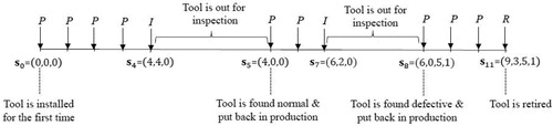
If the retire action is taken, the reward C_r is collected and the end-of-life state $\nabla$ is reached. Figure 2 illustrates a sample path with actions that eventually lead to retiring the tool before its failure. The end-of-life state $\nabla$ is absorbing; i.e., it is a state that, once entered, cannot be left.

Figure 2. Illustration of state transitions where the tool is retired before it fails.

Lifetime value of a tool. Let π be a tool usage policy characterized by taking action $\mu (·)$ every time a decision needs to be made. The expected total reward under this policy when starting in state $\mathbf{s}\in {\mathcal{S}}_0\cup {\mathcal{S}}_1\cup \{\nabla \}$ is given by $$V^{\pi }(\mathbf{s})=\underset{N\to \infty }{\lim }\mathbb{E}\left(\sum _{k=0}^N{g}_{\mu }({\mathbf{s}}_k)|{\mathbf{s}}_0=\mathbf{s}\right),$$ where $g_{\mu }({\mathbf{s}}_k)$ is given by $$g_{\mu }({\mathbf{s}}_k)\mathrm{ }=\{\begin{array}{cc}(1-{\pi }_{f,0}(v,\tau ))(m-{\pi }_d(v+1,\tau +1)C_d)\hfill & \text{for}\mathrm{ }\mu ({\mathbf{s}}_k)=P\mathrm{ }\text{and}\mathrm{ }\mathcal{U}({\mathbf{s}}_k)=0\hfill \\ (1-{\pi }_{f,1}(v,\tau ,w))(m-C_d)\hfill & \text{for}\mathrm{ }\mu ({\mathbf{s}}_k)=P\mathrm{ }\text{and}\mathrm{ }\mathcal{U}({\mathbf{s}}_k)=1\hfill \\ -C_i\hfill & \text{for}\mathrm{ }\mu ({\mathbf{s}}_k)=\mathrm{I}\hfill \\ C_r\hfill & \text{for}\mathrm{ }\mu ({\mathbf{s}}_k)=R\hfill \\ 0\hfill & \text{for}\mathrm{ }{\mathbf{s}}_k=\nabla \hfill \end{array}$$ with $\mathcal{U}({\mathbf{s}}_k)$ denoting the value of the state variable u in ${\mathbf{s}}_k.$ We also refer to $V^{\pi }(\mathbf{s})$ as the lifetime value of a tool at state $\mathbf{s}$ under the policy π; e.g., $V^{\pi }(0,0,0)$ is the lifetime value of a new tool under policy π. Notice that the absorbing end-of-life state must be reached after a finite number of decisions. Therefore, the value function $V^{\pi }(·)$ is guaranteed to be finite. For notational convenience, we let $V(\mathbf{s})$ denote $V^{{\pi }^{*}}(\mathbf{s})$ for ${\pi }^{*}\triangleq \arg {\max }_{\pi }{V}^{\pi }(\mathbf{s}),$ and refer to it as the maximum lifetime value of a tool at state $\mathbf{s}.$ Since the expected total reward of any policy with initial state $\nabla$ is equal to zero, we omit $\nabla$ from the state space of the Markov decision model.

Bellman optimality equations. It can be shown that the maximum lifetime value $V(·)$ satisfies the Bellman optimality equations (Proposition 7.2.1(a) in Bertsekas (2005)): $$V(v,\tau ,w,1)=\max \{V_P(v,\tau ,w,1),C_r\}\forall (v,\tau ,w,1)\in {\mathcal{S}}_1,$$ where $V_P(v,\tau ,w,1)$ is the expected total reward if we take the process action at state $(v,\tau ,w,1)$ and follow the optimal policy thereafter: $$V_P(v,\tau ,w,1)=(1-{\pi }_{f,1}(v,\tau ,w))\left(m-C_d+V(v+1,\tau +1,w,1)\right).$$

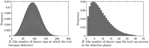
Figure 7. The best-fit probability distributions for the random variables X and H.

Furthermore, the following holds:

$$V(v,\tau ,0)=\{\begin{array}{cc}\max \{V_P(v,\tau ,0),C_r\}\hfill & \forall (v,\tau ,0)\in \{(v,\tau ,0)\in {\mathcal{S}}_0:v<n_X,0<\tau \}\hfill \\ \max \{V_P(v,\tau ,0),V_I(v,\tau ),C_r\}\hfill & \forall (v,\tau ,0)\in \{(v,\tau ,0)\in {\mathcal{S}}_0:v\ge n_X\mathrm{o}r\tau =0\},\hfill \end{array}$$ where $V_P(v,\tau ,0)$ is the expected total reward if we take the process action at state $(v,\tau ,0)$ and follow the optimal policy afterwards; that is to say $$V_P(v,\tau ,0)=(1-{\pi }_{f,0}(v,\tau ))\left(m-{\pi }_d(v+1,\tau +1)C_d+V(v+1,\tau +1,0)\right),$$ and $V_I(v,\tau )$ represents the expected total reward if we take the inspection action at state $(v,\tau ,0)$ and follow the optimal policy afterwards; that is to say $$V_I(v,\tau )=-C_i+{\pi }_d(v,\tau )V(v,0,v-\tau +1,1)+(1-{\pi }_d(v,\tau ))V(v,0,0).$$

We note that there is a special structure of the MDP model that allows us to recursively solve the Bellman equations by making a single pass through the state space at a specific order. Algorithm 1 outlines the details in Section 8.

4. Analysis

4.1. Properties of the probability of being defective and the probability of failure

In this section, we establish the monotonicity properties of the transition probabilities in the MDP model by considering the distributional properties of the random variables X and H. Specifically, Lemma 1 characterizes the probability of being defective and establishes the conditions that guarantee its monotonicity with respect to the cumulative counter.

Lemma 1.

1. The probability of being in the defective phase ${\pi }_d(v,\tau )$ is given by (3) $${\pi }_d(v,\tau )=\frac{\sum _{x=v-\tau +1}^v{f}_X(x){\overline{F}}_H(v-x+1)}{\sum _{x=v-\tau +1}^v{f}_X(x){\overline{F}}_H(v-x+1)+{\overline{F}}_X(v+1)}\forall (v,\tau ,0)\in {\mathcal{S}}_0,$$(3) where the summation is zero for τ = 0.

2. ${\pi }_d(v,\tau )$ is nondecreasing in τ.

3. Let ${\lambda }_X(x)=f_X(x)/{\overline{F}}_X(x)$ for $x\in \{1,\dots ,n_X\}$. If ${\lambda }_X(·)$ is nondecreasing and the property (4) $$\frac{f_X(2)}{f_X(1)}\ge \frac{f_X(3)}{f_X(2)}\ge \dots \ge \frac{f_X(n_X)}{f_X(n_X-1)},$$(4) holds, then ${\pi }_d(v,\tau )$ is nondecreasing in v.

Notice that ${\pi }_d(v,\tau )$ is equal to one for $v\ge n_X$ in Equation (3)(3) $${\pi }_d(v,\tau )=\frac{\sum _{x=v-\tau +1}^v{f}_X(x){\overline{F}}_H(v-x+1)}{\sum _{x=v-\tau +1}^v{f}_X(x){\overline{F}}_H(v-x+1)+{\overline{F}}_X(v+1)}\forall (v,\tau ,0)\in {\mathcal{S}}_0,$$(3) . In Lemma 1(iii), ${\lambda }_X(·)$ is the hazard rate of X; i.e., the conditional probability of defect arrival at the xth product given that the tool has processed x – 1 products in its normal phase. The condition in Equation (4)(4) $$\frac{f_X(2)}{f_X(1)}\ge \frac{f_X(3)}{f_X(2)}\ge \dots \ge \frac{f_X(n_X)}{f_X(n_X-1)},$$(4) is satisfied by many practical distributions such as the discrete uniform distribution, truncated geometric distribution, and truncated discrete Weibull distribution (Nakagawa and Osaki, 1975) with nondecreasing hazard rate. In Lemma 2, we characterize the probability of failure when the tool is last observed as normal, and establish the conditions that guarantee its monotonicity with respect to the run and cumulative counters.

Lemma 2.

1. The probability of failure ${\pi }_{f,0}(v,\tau )$ is given by (5) $${\pi }_{f,0}(v,\tau )=\frac{\sum _{i=0}^{\tau }{f}_X(v+1-i)f_H(i)}{\sum _{i=0}^{\tau }{\overline{F}}_X(v+1-i)f_H(i)+{\overline{F}}_X(v+1-\tau ){\overline{F}}_H(\tau +1)}\forall (v,\tau ,0)\in {\mathcal{S}}_0.$$(5)

2. Let ${\lambda }_H(h)=f_H(h)/{\overline{F}}_H(h)$ for $h\in \{0,1,\dots ,n_H\}$. If ${\lambda }_H(·)$ is nondecreasing, then ${\pi }_{f,0}(v,\tau )$ is nondecreasing in τ.

3. If ${\lambda }_X(·),{\lambda }_H(·)$ and $f_H(·)$ are nondecreasing, and the property in Equation (4)(4) $$\frac{f_X(2)}{f_X(1)}\ge \frac{f_X(3)}{f_X(2)}\ge \dots \ge \frac{f_X(n_X)}{f_X(n_X-1)},$$(4) and the property (6) $$\frac{f_H(1)}{f_H(0)}\ge \frac{f_H(2)}{f_H(1)}\ge \dots \ge \frac{f_H(n_H)}{f_H(n_H-1)},$$(6) hold, then ${\pi }_{f,0}(v,\tau )$ is nondecreasing in v.

In Lemma 2(ii), ${\lambda }_H(h)$ represents the hazard rate of H; i.e., the conditional probability of processing h products in the defective phase given that at least h products have been processed in the defective phase. The condition in Equation (6)(6) $$\frac{f_H(1)}{f_H(0)}\ge \frac{f_H(2)}{f_H(1)}\ge \dots \ge \frac{f_H(n_H)}{f_H(n_H-1)},$$(6) is the counterpart of condition (4) for the random variable of H, and it is satisfied by many of the practical distributions mentioned above. Lemma 2(iii) requires the pmf $f_H(·)$ to be nonincreasing. In practice, a nondecreasing pmf for the random variable H is not uncommon (e.g., when the number of products the tool processes in the defective phase is roughly constant with a uniformly distributed error).

In Lemma 3, we characterize the probability of failure when the tool is last observed as defective, and establish the conditions that guarantee its monotonicity.

Lemma 3.

1. The probability of failure ${\pi }_{f,1}(v,\tau ,w)$ is given by (7) $${\pi }_{f,1}(v,\tau ,w)=\frac{\sum _{x=w}^{v-\tau }{f}_X(x)f_H(v+1-x)}{\sum _{x=w}^{v-\tau }{f}_X(x){\overline{F}}_H(v+1-x)}\forall (v,\tau ,w,1)\in {\mathcal{S}}_1.$$(7)

2. If ${\lambda }_H(·)$ is nondecreasing, then the following results hold: ${\pi }_{f,1}(v,\tau ,w)$ is nondecreasing in τ and nonincreasing in w, and ${\pi }_{f,1}(v,\tau ,w)\ge {\pi }_{f,0}(v,\tau )$ for all $(v,\tau ,w,1)\in {\mathcal{S}}_1.$

3. If ${\lambda }_H(·)$ is nondecreasing and the property in Equation (4)(4) $$\frac{f_X(2)}{f_X(1)}\ge \frac{f_X(3)}{f_X(2)}\ge \dots \ge \frac{f_X(n_X)}{f_X(n_X-1)},$$(4) is satisfied, then ${\pi }_{f,1}(v,\tau ,w)$ is nondecreasing in v.

In the case of dependence between X and H, the closed-form characterizations in Equations (3)(3) $${\pi }_d(v,\tau )=\frac{\sum _{x=v-\tau +1}^v{f}_X(x){\overline{F}}_H(v-x+1)}{\sum _{x=v-\tau +1}^v{f}_X(x){\overline{F}}_H(v-x+1)+{\overline{F}}_X(v+1)}\forall (v,\tau ,0)\in {\mathcal{S}}_0,$$(3) , (5)(5) $${\pi }_{f,0}(v,\tau )=\frac{\sum _{i=0}^{\tau }{f}_X(v+1-i)f_H(i)}{\sum _{i=0}^{\tau }{\overline{F}}_X(v+1-i)f_H(i)+{\overline{F}}_X(v+1-\tau ){\overline{F}}_H(\tau +1)}\forall (v,\tau ,0)\in {\mathcal{S}}_0.$$(5) and (7)(7) $${\pi }_{f,1}(v,\tau ,w)=\frac{\sum _{x=w}^{v-\tau }{f}_X(x)f_H(v+1-x)}{\sum _{x=w}^{v-\tau }{f}_X(x){\overline{F}}_H(v+1-x)}\forall (v,\tau ,w,1)\in {\mathcal{S}}_1.$$(7) can be rewritten by replacing ${\overline{F}}_H(·)$ with ${\overline{F}}_{H|X}(·)$ and by replacing $f_H(·)$ with $f_{H|X}(·),$ which represent the reliability function and pmf of H, respectively, conditional on the realization of X. Finally, it is worth noting that Lemmas 1 to 3 include the sufficient conditions for the monotonicity of the probabilities ${\pi }_d(v,\tau ),{\pi }_{f,0}(v,\tau ),$ and ${\pi }_{f,1}(v,\tau ,w).$ For the analysis of the optimal-policy structure, we will assume that these monotonicity properties hold in Section 4.2 (see Assumptions 1 and 2).

4.2. Structural results on the optimal policy

We separately analyze the structure of the optimal policy for the two cases: when the tool is last observed as being defective (Section 4.2.1) and when the tool is last observed as being normal (Section 4.2.2).

4.2.1. Tool is last observed as being defective (u = 1)

Proposition 1 characterizes the monotonicity properties of the maximum lifetime value of the tool under the following assumption:

Assumption 1.

1. ${\pi }_{f,1}(v,\tau ,w)$ is a nondecreasing function of v.

2. ${\pi }_{f,1}(v,\tau ,w)$ is a nondecreasing function of τ.

3. ${\pi }_{f,1}(v,\tau ,w)$ is a nonincreasing function of w.

Assumption 1 argues that the tool becomes more likely to fail as the product counters increase and the lower bound on X decreases.

Proposition 1.

The maximum lifetime value of a tool has the following properties:

1. $V(v,\tau ,w,1)$ is a nonincreasing function of v and a nonincreasing function of τ.

2. $V(v,\tau ,w,1)$ is a nondecreasing function of w.

Proposition 1 shows that the maximum lifetime value of a tool, which is last observed in a defective phase, gets lower as the cumulative counter increases. This is intuitive, as then fewer products can be processed until the tool failure. Similarly, a higher run counter increases the risks of working with a defective tool and tool failure, reducing the maximum lifetime value. Finally, the higher the inferred lower bound on the realization of X, the higher the maximum lifetime value of the tool. A tool that enters the defective phase later has more potential.

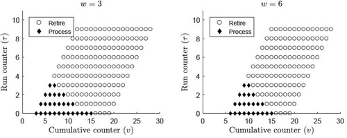
Theorem 1 shows that a threshold-type policy is optimal on each 45° line within the state space ${\mathcal{S}}_1$ at a fixed w. In Figure 3, we visualize the optimal policy when the random variables X and H are uniformly distributed with n_X = 20 and n_H = 10 (i.e., all the conditions of Lemmas 1 to 3 are satisfied). Figure 3 (right) illustrates ${\mathcal{S}}_1$ for w = 6, consisting of 14 (i.e., $n_X-w$) 45° lines. Notice that the difference $v-\tau$ is fixed on each 45° line. It is practically appealing to have a threshold-type policy at a fixed $v-\tau ,$ as then the optimal policy can be viewed in terms of the number of products to process with a defective tool. For the 45° line with $v-\tau =t$ and lower bound w on X, we let $i^{*}(t,w)$ denote the critical threshold that represents the optimal number of products to process with a tool that is just detected as defective.

Figure 3. Optimal policy for u = 1, m = 2, C_r = 10, $C_i=0.5,$ and $C_d=0.1.$

Theorem 1.

Suppose that the last inspection has revealed that the tool is defective.

1. At states $(t+i,i,w,1)\in {\mathcal{S}}_1$, the ‘‘process’’ action is optimal for $i\in \{0,\dots ,i^{*}(t,w)-1\}$ and the ‘‘retire-the-tool’’ action is optimal for $i\in \{i^{*}(t,w),\dots ,n_H-1\}$, where: $$i^{*}(t,w)=\min \{i\in \{0,\dots ,n_H-1\}:{\pi }_{f,1}(t+i,i,w)\ge \frac{m-C_d}{m-C_d+C_r}\},$$ for $t\in \{w,\dots ,n_X-1\}$ and $w\in \{1,\dots ,n_X-1\}.$

2. The critical threshold $i^{*}(t,w)$ is nonincreasing in t and nondecreasing in w.

As an example, notice in Figure 3 (left) that $i^{*}(5,3)=3;$ i.e., it is optimal to take the process action at states $(5+i,i,3,1)$ for i = 0, 1, 2 and it is optimal to take the retire action at states $(5+i,i,3,1)$ for $i=3,4,\dots ,9.$ In Proposition 2, we characterize the maximum lifetime value of a tool that is just found defective; i.e., $V(v,0,w,1).$

Proposition 2.

The maximum lifetime value $V(v,0,w,1)$ of a tool, which has processed at least w products in the normal phase and just been detected as defective by an inspection at cumulative counter v, is given by $$(m-C_d)\sum _{i=1}^{i^{*}(v,w)}\prod _{j=1}^i(1-{\pi }_{f,1}(v+j-1,j-1,w))+C_r\prod _{j=1}^{i^{*}(v,w)}(1-{\pi }_{f,1}(v+j-1,j-1,w)).$$

if $i^{*}(v,w)>0$ and C_r if $i^{*}(v,w)=0.$

The characterization of $V(v,0,w,1)$ in Proposition 2 is in closed form and can easily be calculated after identifying the critical threshold $i^{*}(v,w)$ via Theorem 1. For brevity, we let g(v, w) denote the closed-form characterization of $V(v,0,w,1).$ It will be used in Section 4.2.2 in establishing the conditions for a threshold-type optimal policy structure when the tool is last observed as normal.

4.2.2. Tool is last observed as normal (u = 0)

We start our analysis by characterizing the monotonicity properties of the maximum lifetime value of the tool under the following assumption:

Assumption 2.

1. ${\pi }_{f,0}(v,\tau )$ and ${\pi }_d(v,\tau )$ are nondecreasing functions of v.

2. ${\pi }_{f,0}(v,\tau )$ and ${\pi }_d(v,\tau )$ are nondecreasing functions of τ.

3. ${\pi }_{f,1}(v,\tau ,w)\ge {\pi }_{f,0}(v,\tau )$ for all $(v,\tau ,w,1)\in {\mathcal{S}}_1.$

4. ${\pi }_{f,1}(v+i,0,w+i)$ is nondecreasing in i at a given v and w.

Assumptions 2(i)-(iii) state that the tool becomes more likely to be defective and to fail as the product counters increase, and the probability of tool failure is higher if its last observed phase is defective compared with being normal. Assumption 2(iv) holds if the increase in ${\pi }_{f,1}(v,0,w)$ with a unit increment in v is larger than the increase in ${\pi }_{f,1}(v+1,0,w+1)$ with a unit decrement in w; i.e., ${\pi }_{f,1}(v+1,0,w)-{\pi }_{f,1}(v,0,w)\ge {\pi }_{f,1}(v+1,0,w)-{\pi }_{f,1}(v+1,0,w+1).$

Proposition 3.

The maximum lifetime value of a tool has the following properties:

1. $V(v,\tau ,0)$ is a nonincreasing function of v and a nonincreasing function of τ.

2. $V(v,\tau ,0)\ge V(v,\tau ,w,1)$ for all $(v,\tau ,w,1)\in {\mathcal{S}}_1.$

3. $V(v+i,\tau ,w+i,1)$ is nonincreasing in i.

Propositions 3(i)-(iii) show that the maximum lifetime value of a tool, which is last observed as being normal, gets smaller as the number of products processed by the tool and the number of products since its last inspection increase. Furthermore, it cannot be less than the maximum lifetime value of a tool which is last observed as defective at any cumulative and run counter value. Proposition 3(iii) is implied when the maximum lifetime value of a tool, which is last observed as being defective, is more affected by a unit increase in the cumulative counter than a unit decrease in the lower bound on X.

Similar to Section 4.2.1, we study the structure of the optimal policy on each 45° line within the state space. There is a total of n_X 45° lines in ${\mathcal{S}}_0,$ as illustrated in Figure 4 where n_X = 20. Theorem 2 shows that the optimal policy can be characterized with two critical thresholds on each 45° line within the state space ${\mathcal{S}}_0.$ Specifically, for the 45° line with $v-\tau =t,$ where the possible states are $(t+i,i,0)$ for $i\in \{0,1,\dots ,n_X+n_H-1-t\},$ the optimal action is as follows: process the next product if $i<{\mathcal{\ell }}^{*}(t),$ inspect the tool if ${\mathcal{\ell }}^{*}(t)\le i<u^{*}(t),$ and retire the tool if $i\ge u^{*}(t).$ Notice that ${\mathcal{\ell }}^{*}(t)$ also represents the optimal number of products to process with a tool that is just inspected and found to be normal.

Figure 4. Optimal policy for u = 0 considering the same instance as in Figure 3 with C_r = 20.

Theorem 2.

Let $$r(v)\triangleq m (\mathbb{E}(X|X>v)-v-1)+(\mathbb{E}(H)+1)(m-C_d)$$ for

$$v\in \{0,\dots ,n_X-1\},{\Delta }_d(v,\tau ;a,b)\triangleq {\pi }_d(v,\tau )-{\pi }_d(v-a,\tau -b),$$

and $${\Delta }_f(v,\tau ;a,b)\triangleq {\pi }_{f,0}(v,\tau )-{\pi }_{f,0}(v-a,\tau -b).$$

Suppose that the last inspection has revealed that the tool is in the normal phase:

1. For $t\in \{0,\dots ,n_X-1\}$, there exists a critical threshold $u^{*}(t)$ such that the ‘‘retire-the-tool’’ action is optimal at states $(t+i,i,0)\in {\mathcal{S}}_0$ for $i\in \{u^{*}(t),\dots ,n_X+n_H-1-t\}.$

2. There exists a critical threshold ${\mathcal{\ell }}^{*}(t)$ such that the ‘‘process’’ action is optimal at states $(t+i,i,0)\in {\mathcal{S}}_0$ for $i\in \{0,\dots ,{\mathcal{\ell }}^{*}(t)-1\}$ assuming that the condition: (8) $$\begin{array}{c}{C}_i+{\Delta }_f(n_X,n_X-t;1,1)(m-C_d+C_r)+C_r{\pi }_d(n_X-1,n_X-t-1)\\ \ge {\pi }_d(n_X-1,n_X-t-1)g(n_X-1,t+1)+(1-{\pi }_d(n_X-1,n_X-t-1))r(n_X-1)\end{array}$$(8)

holds if $t\in \{0,\dots ,n_X-2\}$ and the condition: (9) $$\begin{array}{c}{\Delta }_f(v,\tau ;1,1)(C_r+m)+({\pi }_d(v-1,\tau -1)+{\Delta }_d(v+1,\tau +1;1,1)+{\pi }_{f,0}(v-1,\tau -1){\pi }_d(v,\tau ))C_d\\ \ge {\Delta }_d(v,\tau ;1,1)(r(v)+C_r-g(v,v-\tau +1))+m+{\pi }_{f,0}(v,\tau ){\pi }_d(v+1,\tau +1)C_d\end{array}$$(9)

holds for all $(v,\tau )\in \{(t+i,i):i=1,\dots ,n_X-1-t\}$ if $t\in \{0,\dots ,n_X-3\}$. For $t=n_X-1,{\mathcal{\ell }}^{*}(t)$ is equal to $u^{*}(t).$

The condition (8(8) $$\begin{array}{c}{C}_i+{\Delta }_f(n_X,n_X-t;1,1)(m-C_d+C_r)+C_r{\pi }_d(n_X-1,n_X-t-1)\\ \ge {\pi }_d(n_X-1,n_X-t-1)g(n_X-1,t+1)+(1-{\pi }_d(n_X-1,n_X-t-1))r(n_X-1)\end{array}$$(8) ) guarantees if the process action is optimal at state $(n_X,\tau ,0)$ then it is also optimal at state $(n_X-1,\tau -1,0).$ Similarly, the condition (9(9) $$\begin{array}{c}{\Delta }_f(v,\tau ;1,1)(C_r+m)+({\pi }_d(v-1,\tau -1)+{\Delta }_d(v+1,\tau +1;1,1)+{\pi }_{f,0}(v-1,\tau -1){\pi }_d(v,\tau ))C_d\\ \ge {\Delta }_d(v,\tau ;1,1)(r(v)+C_r-g(v,v-\tau +1))+m+{\pi }_{f,0}(v,\tau ){\pi }_d(v+1,\tau +1)C_d\end{array}$$(9) ) guarantees that if the process action is optimal at state $(v,\tau ,0)$ then it is also optimal at state $(v-1,\tau -1,0)$ for $v<n_X.$ These conditions relate the economic parameters with the rate of increase in the probability of failure and the probability of being defective. In our numerical experiments, the conditions (8(8) $$\begin{array}{c}{C}_i+{\Delta }_f(n_X,n_X-t;1,1)(m-C_d+C_r)+C_r{\pi }_d(n_X-1,n_X-t-1)\\ \ge {\pi }_d(n_X-1,n_X-t-1)g(n_X-1,t+1)+(1-{\pi }_d(n_X-1,n_X-t-1))r(n_X-1)\end{array}$$(8) ) and (9(9) $$\begin{array}{c}{\Delta }_f(v,\tau ;1,1)(C_r+m)+({\pi }_d(v-1,\tau -1)+{\Delta }_d(v+1,\tau +1;1,1)+{\pi }_{f,0}(v-1,\tau -1){\pi }_d(v,\tau ))C_d\\ \ge {\Delta }_d(v,\tau ;1,1)(r(v)+C_r-g(v,v-\tau +1))+m+{\pi }_{f,0}(v,\tau ){\pi }_d(v+1,\tau +1)C_d\end{array}$$(9) ) are always satisfied for the probability distributions of X and H estimated from real-world data and under realistic cost parameters, and hence, we consider them as mild sufficient conditions. Figure 4 illustrates the critical thresholds ${\mathcal{\ell }}^{*}(t)$ and $u^{*}(t)$ for $t=0,\dots ,n_X-1;$ e.g., ${\mathcal{\ell }}^{*}(0)=10$ and $u^{*}(0)=18,$ or ${\mathcal{\ell }}^{*}(17)=u^{*}(17)=2.$ Next, we establish the monotonicity of the critical thresholds.

Theorem 3.

For $t\in \{0,\dots ,n_X-2\}$, the following results hold: (i) $u^{*}(t)\ge u^{*}(t+1).$

(ii) ${\mathcal{\ell }}^{*}(t)\ge {\mathcal{\ell }}^{*}(t+1)$ if (10) $$\begin{array}{c}{C}_i+{\Delta }_f(n_X,n_X-t-1;1,0)(m-C_d+C_r)+C_r{\pi }_d(n_X-1,n_X-t-1)\\ \ge {\pi }_d(n_X-1,n_X-t-1)g(n_X-1,t+1)+(1-{\pi }_d(n_X-1,n_X-t-1))r(n_X-1)\end{array}$$(10) and the condition: (11) $$\begin{array}{c}{\Delta }_f(v,\tau ;1,0)(C_r+m)+({\pi }_d(v-1,\tau )+{\Delta }_d(v+1,\tau +1;1,0)+{\pi }_{f,0}(v-1,\tau ){\pi }_d(v,\tau +1))C_d\\ \ge {\Delta }_d(v,\tau ;1,0)(r(v)+C_r-g(v,v-\tau +1))+m+{\pi }_{f,0}(v,\tau ){\pi }_d(v+1,\tau +1)C_d\end{array}$$(11) is satisfied for all $(v,\tau )\in \{(n_X-i,n_X-t-i-1):i=1,\dots ,n_X-2-t\}.$

Theorem 3(i) shows that the critical threshold $u^{*}(t)$ never increases as t increases. However, it is not always the case for ${\mathcal{\ell }}^{*}(t)$ (see Figure 4). Theorem 3(ii) establishes the conditions under which the critical threshold ${\mathcal{\ell }}^{*}(t)$ is guaranteed to be nonincreasing in t. The condition (10(10) $$\begin{array}{c}{C}_i+{\Delta }_f(n_X,n_X-t-1;1,0)(m-C_d+C_r)+C_r{\pi }_d(n_X-1,n_X-t-1)\\ \ge {\pi }_d(n_X-1,n_X-t-1)g(n_X-1,t+1)+(1-{\pi }_d(n_X-1,n_X-t-1))r(n_X-1)\end{array}$$(10) ) is the counterpart of condition (8(8) $$\begin{array}{c}{C}_i+{\Delta }_f(n_X,n_X-t;1,1)(m-C_d+C_r)+C_r{\pi }_d(n_X-1,n_X-t-1)\\ \ge {\pi }_d(n_X-1,n_X-t-1)g(n_X-1,t+1)+(1-{\pi }_d(n_X-1,n_X-t-1))r(n_X-1)\end{array}$$(8) ), and ensures that if the process action is optimal at state ($n_X,\tau ,0$) then it is also optimal at state $(n_X-1,\tau ,0).$ Similarly, the condition (11(11) $$\begin{array}{c}{\Delta }_f(v,\tau ;1,0)(C_r+m)+({\pi }_d(v-1,\tau )+{\Delta }_d(v+1,\tau +1;1,0)+{\pi }_{f,0}(v-1,\tau ){\pi }_d(v,\tau +1))C_d\\ \ge {\Delta }_d(v,\tau ;1,0)(r(v)+C_r-g(v,v-\tau +1))+m+{\pi }_{f,0}(v,\tau ){\pi }_d(v+1,\tau +1)C_d\end{array}$$(11) ) is the counterpart of condition (9(9) $$\begin{array}{c}{\Delta }_f(v,\tau ;1,1)(C_r+m)+({\pi }_d(v-1,\tau -1)+{\Delta }_d(v+1,\tau +1;1,1)+{\pi }_{f,0}(v-1,\tau -1){\pi }_d(v,\tau ))C_d\\ \ge {\Delta }_d(v,\tau ;1,1)(r(v)+C_r-g(v,v-\tau +1))+m+{\pi }_{f,0}(v,\tau ){\pi }_d(v+1,\tau +1)C_d\end{array}$$(9) ) for $v<n_X,$ and ensures that if the process action is optimal at state $(v,\tau ,0)$ then it is also optimal at state $(v-1,\tau ,0).$

5. Numerical analysis

The objective of this section is to provide managerial insights on: (i) how the maximum lifetime value of a new tool is affected by various economic and degradation-related parameters; (ii) the benefit of the optimal tool-usage policy compared with the fixed-threshold policy, i.e., the benchmark policy from practice; and (iii) what portion of this benefit come from postponing the retirement of a defective tool. We let m be equal to one and consider various values for each cost parameter. We consider that X is uniformly distributed on $\{1,\dots ,n_X\};$ i.e., $f_X(x)=1/n_X$ for $x=1,\dots ,n_X.$ This distribution implies that the tool enters at the defective phase at any product from one to n_X with equal probability. In the remainder of this section, we let n_X = 32. The random variable H is uniformly distributed on $\{n_H-\delta +1,\dots ,n_H\};$ i.e., $f_H(n_H+1-i)=1/\delta$ if $i=1,\dots ,\delta$ and $f_H(i)=0,$ otherwise. That is, the number of product the tool processes in the defective phase has varying levels of uncertainty controlled by parameter δ. We let $n_H\in \{8,16,32\}$ and consider three cases: The distribution H1 has δ = 1, the distribution H2 has $\delta =n_H/2,$ and the distribution H3 has $\delta =n_H.$ The distribution H1 represents that a defective tool processes a constant number of products. As we go from distribution H1 to H3, the mean decreases and the variability increases. Although we focus on stylized distribution functions in this section, we will consider the more flexible discrete Weibull distribution in Section 6 and estimate its parameters from real-world maintenance logs as described in Section EC.3.

5.1. The impact of cost parameters on the maximum lifetime value

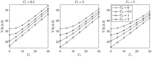
Figure 5 illustrates the increase in the maximum lifetime value of a new tool as the salvage reward C_r increases. We make three key observations. First, the distinction between the cases with different C_d values becomes more visible for lower C_r. At high C_r values, it is tempting not to use a defective tool at all, and the value of C_d has no effect. Second, as C_r increases, the rate of increase in maximum lifetime value increases and then stabilizes. This means, $V(0,0,0)-C_r$ (which represents the production value of a tool) decreases at a diminishing rate as C_r increases. In theory, if C_r approaches a very large number, then the production value of the tool would be zero (because then it would be optimal to retire the tool immediately without taking any risk of failure). Third, C_i influences the maximum lifetime value when C_r is sufficiently high. This is intuitive because if C_r is sufficiently high, then it makes sense to use the tool only if we know it is not close to failure, and in this situation, inspection is instrumental under the optimal policy.

Figure 5. Maximum lifetime value of a new tool for the distribution H2 with n_H = 16.

5.2. Comparison with the optimal fixed-threshold policy

We let V_ft denote the lifetime value of a new tool under the optimal fixed-threshold policy; see Section 1 for details on the fixed-threshold policy. In Tables 2 to 4, we let n_H = 32 and compare the values of V_ft with $V(0,0,0)$ under various cost parameters and the distributions H1, H2, and H3. To make the comparison easier, we also report Δ_ft, which is the relative improvement over the optimal fixed threshold policy; i.e., ${\Delta }_{ft}=(V(0,0,0)-V_{ft})/V_{ft}.$ We observe that the difference between the lifetime values of a new tool under the optimal tool-usage policy and the optimal fixed-threshold policy can be substantial. For example, when C_r = 10, C_i = 1, and C_d = 0, the percentage improvement Δ_ft is equal to 38.2% for the distribution H1 (Table 2), and it is equal to 18.8% and 8.4% for the distributions H2 and H3, respectively (Tables 3 and 4).

Table 2. Comparison of the lifetime values of a new tool for the distribution H1 with n_H = 32.

		Cr = 5				Cr = 10				Cr = 20
$C_i/C_r$	Cd	Vft	Vnp	$V(0,0,0)$	Δft (%)	Vft	Vnp	$V(0,0,0)$	Δft (%)	Vft	Vnp	$V(0,0,0)$	Δft (%)
0.05	0	35.8	37.0	52.8	47.8	40.5	42.0	56.6	39.6	50.0	52.0	64.8	29.6
	0.5	30.6	31.3	38.2	25.1	35.3	36.3	42.4	20.0	44.8	46.3	51.2	14.3
	1	25.4	25.7	25.7	1.0	30.2	30.7	30.7	1.7	39.7	40.7	40.7	2.5
	2	21.2	21.8	21.8	2.7	25.3	26.1	26.1	3.3	33.8	35.1	35.1	3.8
0.1	0	35.5	37.0	52.5	47.9	40.0	42.0	55.3	38.2	49.0	52.0	62.6	27.8
	0.5	30.3	31.3	37.7	24.4	34.8	36.3	41.4	19.0	43.8	46.3	49.8	13.6
	1	25.2	25.7	25.7	2.0	29.7	30.7	30.7	3.4	38.7	40.7	40.7	5.2
	2	20.3	21.1	21.1	4.1	23.8	25.1	25.1	5.4	32.2	34.3	34.3	6.8
0.2	0	35.0	37.0	52.5	50.0	39.0	42.0	54.4	39.5	47.0	52.0	60.4	28.4
	0.5	29.8	31.3	37.5	25.8	33.8	36.3	40.5	19.8	41.8	46.3	48.6	16.1
	1	24.7	25.7	25.7	4.1	28.7	30.7	30.7	7.0	36.7	40.7	40.7	10.9
	2	18.8	20.1	20.1	6.8	22.2	24.3	24.3	9.8	30.2	34.3	34.3	13.9

Table 3. Comparison of the lifetime values of a new tool for the distribution H2 with n_H = 32.

		Cr = 5				Cr = 10				Cr = 20
$C_i/C_r$	Cd	Vft	Vnp	$V(0,0,0)$	Δft (%)	Vft	Vnp	$V(0,0,0)$	Δft (%)	Vft	Vnp	$V(0,0,0)$	Δft (%)
0.05	0	35.0	36.1	44.5	27.2	39.4	40.6	46.2	17.4	48.1	49.6	53.0	10.2
	0.5	30.0	30.6	33.4	11.4	34.4	35.1	36.7	6.8	43.1	44.2	45.1	4.5
	1	25.2	25.3	25.3	0.4	29.9	29.9	29.9	0.1	39.4	39.4	39.4	0.1
	2	21.2	21.8	21.8	2.7	25.3	26.1	26.1	3.3	33.8	35.1	35.1	3.8
0.1	0	34.8	36.1	44.5	28.0	38.9	40.6	46.2	18.8	47.2	49.6	52.1	10.4
	0.5	29.8	30.6	33.4	12.3	33.9	35.1	36.4	7.2	42.2	44.2	44.3	4.9
	1	24.9	25.3	25.3	1.4	29.4	29.9	29.9	1.8	38.4	39.4	39.4	2.7
	2	20.3	21.1	21.1	4.1	23.8	25.1	25.1	5.4	32.1	34.2	34.2	6.6
0.2	0	34.3	36.1	44.5	29.7	38.0	40.6	46.2	21.7	45.3	49.6	52.1	14.9
	0.5	29.3	30.6	33.4	14.0	33.0	35.1	36.4	10.2	40.4	44.2	44.3	9.7
	1	24.4	25.3	25.3	3.4	28.4	29.9	29.9	5.4	36.4	39.4	39.4	8.4
	2	18.8	20.1	20.1	6.8	22.1	24.3	24.3	9.7	30.1	34.2	34.2	13.7

Table 4. Comparison of the lifetime values of a new tool for the distribution H3 with n_H = 32.

		Cr = 5				Cr = 10				Cr = 20
$C_i/C_r$	Cd	Vft	Vnp	$V(0,0,0)$	Δft (%)	Vft	Vnp	$V(0,0,0)$	Δft (%)	Vft	Vnp	$V(0,0,0)$	Δft (%)
0.05	0	31.5	32.1	36.3	15.5	34.7	35.4	37.2	7.3	41.1	41.8	41.8	1.7
	0.5	27.7	28.0	28.9	4.6	30.9	31.2	31.2	1.1	38.3	38.4	38.4	0.4
	1	24.3	24.4	24.4	0.4	28.1	28.3	28.3	1.0	35.6	36.5	36.5	2.4
	2	21.1	21.7	21.7	3.0	24.7	25.7	25.7	4.0	32.1	33.9	33.9	5.6
0.1	0	31.3	32.1	36.3	16.1	34.3	35.4	37.2	8.4	40.4	41.8	41.8	3.4
	0.5	27.5	28.0	28.9	5.2	30.6	31.2	31.2	2.3	37.4	38.4	38.4	2.7
	1	24.1	24.2	24.2	0.4	27.6	27.9	27.9	1.0	34.8	36.0	36.0	3.5
	2	20.1	21.0	21.0	4.5	23.2	24.7	24.7	6.6	29.7	32.9	32.9	10.6
0.2	0	31.0	32.1	36.3	17.4	33.7	35.4	37.2	10.6	39.1	41.8	41.8	7.0
	0.5	27.2	28.0	28.9	6.5	29.9	31.2	31.2	4.6	35.7	38.4	38.4	7.6
	1	23.6	24.2	24.2	2.2	26.8	27.9	27.9	4.3	33.0	36.0	36.0	9.0
	2	18.8	20.1	20.1	7.2	21.4	23.9	23.9	11.4	27.7	32.9	32.9	18.7

We make two observations regarding the sensitivity of the percentage improvement Δ_ft. First, how Δ_ft changes with C_r depends on the value of C_d. To be specific, we note that Δ_ft decreases in C_r for low values of C_d. As C_r increases, it becomes less important to postpone the retirement of a defective tool (because the optimal policy tends to retire the tool earlier to save the high salvage reward). Also, if C_d is low, it matters less whether to inspect the tool at fixed or adaptive thresholds. Thus, the two advantages of the optimal tool-usage policy over the fixed-threshold policy disappear, and we observe that Δ_ft decreases in C_r for lower values of C_d. On the other hand, when C_d is high enough, optimally timing the inspection moments becomes also important, and Δ_ft does not necessarily decrease in C_r. Second, we observe that Δ_ft increases as C_i increases for sufficiently high values of C_d. This is the situation in which working with a defective tool is costly and inspections are therefore important. As the cost of inspection increases, it becomes critical to adaptively plan what triggers an inspection, and hence, the improvement potential of the optimal tool usage policy is larger.

5.3. The value of postponing the tool replacement in the defective phase

In order to assess the value of postponing the retire-the-tool action in the defective phase, we further compare the maximum lifetime value under the optimal tool-usage policy with the lifetime value under the same policy except with one difference: the retire-the-tool action is taken as soon as an inspection finds the tool defective. We denote the lifetime value of a new tool under this no-postponement policy with V_np. The difference $V_{np}-V_{ft}$ can be interpreted as the value of optimally timing the inspection moments, and the difference $V(0,0,0)-V_{np}$ can be interpreted as the value of postponing the retire action for a defective tool. We observe in Tables 2 to 4 that the difference $V(0,0,0)-V_{np}$ is the most noticeable for lower C_d and C_r values.

5.4. The impact of the distribution of H on the maximum lifetime value

The expected number of defective products processed with a defective tool is the highest for the distribution H1 (Table 2) and the lowest for the distribution H3 (Table 4). This explains why the maximum lifetime values are the highest in Table 2 and lowest in Table 4. The results for the distribution H3 with n_H = 16 and for the distribution H1 with n_H = 8 are reported in Table 5(a) and Table 5(b), respectively. Notice that the mean values of these two distributions are very close to each other, with the former having a larger variability than the latter. The decrease in the lifetime values under all the policies can be attributable to the higher variability in the distribution of H3.

Table 5. Comparison of the lifetime values of a new tool under different policies for C_r = 20:

(a) The distribution H3.

		Cr = 5				Cr = 10				Cr = 20
$C_i/C_r$	Cd	Vft	Vnp	$V(0,0,0)$	Δft (%)	Vft	Vnp	$V(0,0,0)$	Δft (%)	Vft	Vnp	$V(0,0,0)$	Δft (%)
8	0	31.6	33.6	33.6	6.5	29.6	32.7	32.7	10.6	28.6	32.7	32.7	14.2
	0.5	30.7	33.0	33.0	7.6	28.2	32.1	32.1	13.8	27.3	32.1	32.1	17.7
	1	29.8	32.4	32.4	8.8	26.8	31.5	31.5	17.5	25.9	31.5	31.5	21.7
	2	28.0	31.4	31.4	12.0	24.2	30.6	30.6	26.1	23.2	30.6	30.6	31.7
16	0	36.4	37.0	37.0	1.8	35.4	36.1	36.1	2.0	34.0	36.1	36.1	6.3
	0.5	34.7	35.8	35.8	3.2	33.3	34.8	34.8	4.5	31.8	34.7	34.7	9.0
	1	33.1	34.7	34.7	4.7	31.1	33.6	33.6	7.9	29.7	33.5	33.5	13.0
	2	30.6	32.9	32.9	7.6	27.8	31.8	31.8	14.5	25.4	31.7	31.7	24.7

(b) The distribution H1.

		$C_i/C_r=0.05$				$C_i/C_r=0.1$				$C_i/C_r=0.2$
nH	Cd	Vft	Vnp	$V(0,0,0)$	Δft (%)	Vft	Vnp	$V(0,0,0)$	Δft (%)	Vft	Vnp	$V(0,0,0)$	Δft (%)
8	0	40.1	41.0	41.1	2.6	37.5	38.9	38.9	3.8	36.1	36.6	36.6	1.1
	0.5	38.5	39.2	39.2	1.8	35.3	37.1	37.1	5.2	33.8	34.9	34.9	3.4
	1	36.9	37.5	37.5	1.5	33.7	35.5	35.5	5.5	31.4	33.7	33.7	7.3
	2	33.7	34.7	34.7	2.8	30.5	32.9	32.9	7.6	26.6	31.7	31.7	19.1

6. Case study: Managing ECM tools at Philips Consumer Lifestyle

The case study was conducted at the manufacturing plant of Philips Consumer Lifestyle (PCL) in Drachten, the Netherlands. The plant in Drachten produces highly-precise shaver caps (Figure 6, right) for electric shavers by using a micro-machining process called ECM. The ECM process (Figure 6, left) requires expensive machine tools that have an intricate surface to mirror the required geometrics of the shaver cap. The objective of our collaboration with PCL is to design an improved tool-usage policy that maximizes the economic potential of each ECM tool. The current tool-usage strategy at PCL is based on the fixed-threshold policy as described in Section 1. When the wear on the tool surface is less than a specific value, the tool is regarded as being healthy. However, if the tool wear exceeds this specific value, then the tool is still operational but produces faulty products, and hence, it is regarded as defective. The defective state of the tool can only be detected with an inspection performed by specialized equipment and technicians. If a defective tool continues production, it eventually fails, due to the accumulation of wear. A failure substantially reduces the economic value of the tool.

Figure 6. Illustration of the ECM process.

After analyzing the maintenance logs between January 2015 and February 2017, we identify 49 tools for further analysis based on the availability and similar characteristics of their data. In Table 6, we provide a sample of the maintenance logs. The data include the run counter and cumulative counter values of an individual tool after each production run, as well as the reason for removing the tool from a machine and the follow-up maintenance activity. The maintenance logs do not keep track of the wear level on the tool surface.

Table 6. Example of the maintenance logs on ECM tools (note that the format in this table is day-month-year).

Tool ID	Machine	Time the tool is put on	Time the tool is taken off	Run counter	Cumulative counter	Reason the tool is taken off	Maintenance activity
Y889	GE1C	13-12-16 21:36	22-12-16 19:55	16 863	159 610	NDEF	ELST
Y948	GE1E	3-08-15 9:09	22-08-15 10:24	36 903	154 980	VGL3	ELST
Y934	GE1F	13-01-17 12:22	7-02-17 20:02	49 912	158 564	MASB	ELST
Y933	GE1A	18-12-16 9:07	18-12-16 11:44	5013	64 814	H134	ELSL
Y894	GE1G	13-11-15 16:36	19-11-15 0:39	6107	14 158	K264	EL2X
Y932	GE1B	8-02-15 8:10	15-02-15 0:58	14 342	23 056	VGL3	ELBE
…	…	…	…	…	…	…	…

By tracking the reason why a tool has been taken off the production and the subsequent maintenance activity, we categorize each tool in one of the following four groups:

1. The tool is found normal in the last inspection, and it has not failed yet by the time it is retired.

2. The tool is found normal in the last inspection, and it has failed afterwards.

3. The tool is found defective in the last inspection, and it has not failed yet by the time it is retired.

4. The tool is found defective in the last inspection and it has failed afterwards. Specifically, if a tool’s last inspection has resulted in a maintenance activity that includes just cleaning the tool, the tool is regarded as ‘‘last observed as healthy’’, corresponding to groups 1 and 2.

By matching the reason the tool is last taken off the production with the four-digid error code that represents the tool failure, we conclude that 24 tools are in group 1 and 14 tools are in group 2. On the other hand, if a tool’s last inspection has resulted in more than just cleaning the tool, we regard them as ‘‘last observed as defective.’’ After matching the reason the tool is last taken off the production with the failure code, we find that seven tools are in group 3 and 4 tools are in group 4.

In Section EC.3, we provide the details on how we combine the data belonging to each group to estimate the probability distributions of the random variables X and H in our model. For ease in computations, we divide the run counter and cumulative counter by 1000, and then round them to the nearest integer. We assume that the random variables X and H both follow a discrete Weibull distribution (Nakagawa and Osaki, 1975), and estimate the scale parameter of X as $5.52\times {10}^{-7}$ and the shape parameter of X as 3.1056. We estimate the scale and shape parameters of H as 0.0453 and 1.3833, respectively. The resulting distributional shapes of the random variables X and H are illustrated in Figure 7.

Finally, we compare the maximum lifetime value of a new ECM tool under the optimal tool usage policy (i.e., $V(0,0,0)$) to the lifetime value under the optimal fixed-threshold policy (i.e., V_ft), and report their percentage difference Δ_ft in Table 7. Since the fixed-threshold policy used in practice is not necessarily the optimal one, our comparison can be considered as a lower bound on the economic benefit of the optimal tool usage policy in practice. For confidentiality, we do not disclose the economic parameters but run our experiments with a large set of representative cost values. We also do not specify the fixed-threshold policy parameters used by PCL. Table 7 shows that, depending on the cost parameters, the percentage improvement over the optimal fixed-threshold policy can take values from 5.2% to 20.7%.

Table 7. The values of Δ_ft (unit: %) calculated for a new ECM tool.

$C_d/m$	$C_i=1\%$ of Cr	$C_i=5\%$ of Cr	$C_i=10\%$ of Cr	$C_i=20\%$ of Cr
0.00	5.2	8.5	7.8	9.6
0.25	5.7	9.6	8.8	10.7
0.50	6.2	10.5	9.9	11.8
0.75	6.8	11.0	11.1	13.1
1.00	7.4	11.6	12.3	14.4
1.25	8.0	12.2	13.6	15.8
1.50	8.7	12.8	15.1	17.4
1.75	9.4	13.4	16.5	19.0
2.00	10.1	14.2	18.1	20.7

7. Conclusion

We study the inspection and retirement decisions for machine tools that go through a hidden defective phase that can only be detected via costly inspections. In particular, we identify the right moment to inspect and retire the tool such that the net expected production reward obtained from a specific tool is maximized. The products processed by a defective tool do not necessarily generate the same reward obtained from a normal tool and a tool failure can be very costly. We establish the structural properties of the optimal policy as a function of practical product counters, the last observed degradation phase of the tool and an inferred lower bound on the numbers of products the tool has processed in its normal phase. The structural properties depend on mild conditions on economic parameters as well as the probability distributions of the number of products the machine tool processes in the normal and defective phases. Therefore, the existence of structural properties can easily be verified in practice after estimating these probability distributions. The implementation of our model by using the real-world maintenance logs at PCL shows that the value of the optimal tool usage policy can be substantial compared with the current alternative. A future research direction is to develop the optimal tool usage policy that takes the advantage of coordinating the inspection decisions for multiple tools in order to maximize their total lifetime value. Another potential research direction is to jointly optimize the usage policy of the tools and the procurement decisions of the spare tools on the production line.

Acknowledgments

The authors would like to thank Bas Tijsma from Philips Consumer Lifestyle for his valuable input in model development and data analysis.

Additional information

Funding

The authors gratefully acknowledge the financial support by European Commission H2020-ECSEL Project MANTIS-662189.

Notes on contributors

Alp Akcay

Alp Akcay is an assistant professor in the Department of Industrial Engineering and Innovation Sciences at Eindhoven University of Technology. He received his Ph.D. in Operations Management from the Tepper School of Business at Carnegie Mellon University. His research interests include statistical decision making under uncertainty, simulation design and analysis, and approximate dynamic programming with applications such as planning and control of manufacturing systems and predictive maintenance for capital goods.

Engin Topan

Engin Topan is an assistant professor of reliability, maintenance, and service logistics at the University of Twente. He received his Ph.D. from the Middle East Technical University, Turkey, in 2010. He worked at different positions at Cankaya University, Turkish Military Academy, Erasmus University Rotterdam, and Eindhoven University of Technology. He took part in several projects on after sales service logistics and maintenance planning for capital goods. His research interests include spare parts and service logistics, and maintenance panning.

Geert-Jan van Houtum

Geert-Jan van Houtum is a professor of maintenance and reliability at the Department of Industrial Engineering and Innovation Sciences, Eindhoven University of Technology. His research is focused on predictive maintenance, availability management of capital goods, spare parts management, and the effect of design decisions on the total cost of ownership of capital goods. Much of his research is based on a close collaboration with e.g. ASML, Dutch Railways, Philips, and the Royal Airforce. He is associate editor of Manufacturing and Service Operations Management and area editor at Service Science.

References

- Arts, J. and Basten, R. (2018) Design of multi-component periodic maintenance programs with single-component models. IISE Transactions, 50, 606–615.
- Barlow, R.E., Hunter, L.C. and Proschan, F. (1963) Optimum checking procedures. Journal of the Society for Industrial and Applied Mathematics, 11, 1078–1095.
- Berrade, M.D., Scarf, P.A. and Cavalcante, C.A.V. (2017) A study of postponed replacement in a delay time model. Reliability Engineering & System Safety, 168, 70–79.
- Bertsekas, D.P. (2005) Dynamic Programming and Optimal Control, vol. 1. 4th ed. Athena Scientific, Belmont, MA.
- Bertsekas, D.P. and Tsitsiklis, J.N. (1991) An analysis of stochastic shortest path problems. Mathematics of Operations Research, 16, 580–595.
- Christer, A.H. (1982) Modelling inspection policies for building maintenance. Journal of the Operational Research Society, 33, 723–732.
- Christer, A.H. and Wang, W. (1995) A simple condition monitoring model for a direct monitoring process. European Journal of Operational Research, 82, 258–269.
- de Jonge, B. and Scarf, P.A. (2019) A review on maintenance optimization. European Journal of Operational Research. doi:10.1016/j.ejor.2019.09.047.
- Duan, C., Makis, V. and Deng, C. (2019) Optimal Bayesian early fault detection for CNC equipment using hidden semi-Markov process. Mechanical Systems and Signal Processing, 122, 290–306.
- Groover, M.P. (2017) Groover’s principles of modern manufacturing: materials, processes, and systems, John Wiley & Sons, Inc., Hoboken, NJ.
- Jiang, R. (2017) An efficient quasi-periodic inspection scheme for a one-component system. IMA Journal of Management Mathematics, 28, 373–386.
- Kaio, N. and Osaki, S. (1984) Some remarks on optimum inspection policies. IEEE Transactions on Reliability, 33, 277–279.
- Khojandi, A., Maillart, L.M. and Prokopyev, O.A. (2014) Optimal planning of life-depleting maintenance activities. IIE Transactions, 46, 636–652.
- Kim, M.J. and Makis, V. (2013) Joint optimization of sampling and control of partially observable failing systems. Operations Research, 61, 777–790.
- Leung, F.K. (2001) Inspection schedules when the lifetime distribution of a single-unit system is completely unknown. European Journal of Operational Research, 132, 106–115.
- MacPherson, A.J. and Glazebrook, K.D. (2011) A dynamic programming policy improvement approach to the development of maintenance policies for 2-phase systems with aging. IEEE Transactions on Reliability, 60, 448–459.
- Maillart, L.M., (2006) Maintenance policies for systems with condition monitoring and obvious failures. IIE Transactions, 38, 463–475.
- Maillart, L.M. and Pollock, S.M. (2002) Cost-optimal condition-monitoring for predictive maintenance of 2-phase systems. IEEE Transactions on Reliability, 51, 322–330.
- Makis, V. and Jiang, X. (2003) Optimal replacement under partial observations. Mathematics of Operations Research, 28, 382–394.
- Moghaddass, R. and Ertekin, S. (2018) Joint optimization of ordering and maintenance with condition monitoring data. Annals of Operations Research, 263, 271–310.
- Nakagawa, T. and Osaki, S. (1975) The discrete Weibull distribution. IEEE Transactions on Reliability, 24, 300–301.
- Ohnishi, M., Kawai, H. and Mine, H. (1986) An optimal inspection and replacement policy for a deteriorating system. Journal of Applied Probability, 23, 973–988.
- Ozekici, S. and Pliska, S.R. (1991) Optimal scheduling of inspections: A delayed Markov model with false positives and negatives. Operations Research, 36, 261–273.
- Parmigiani, G. (1996) Optimal scheduling of fallible inspections. Operations Research, 44, 360–367.
- Probst, E. (2015) 6 factors maximize profitability in high-precision machining. www.mmsonline.com/articles/6-factors-help-maximize-profitability-in-high-precision-machining. Accessed July 15, 2018.
- Scarf, P.A., Cavalcante, C., Dwight, R.A. and Gordon, P. (2009) An age-based inspection and replacement policy for heterogeneous components. IEEE Transactions on Reliability, 58, 641–648.
- Sengupta, B. (1980) Inspection procedures when failure symptoms are delayed. Operations Research, 28, 768–776.
- Van Oosterom, C.D., Elwany, A.H., Çelebi, D. and van Houtum, G. (2014) Optimal policies for a delay time model with postponed replacement. European Journal of Operational Research, 232, 186–197.
- Wang, W. (2012) An overview of the recent advances in delay-time-based maintenance modelling. Reliability Engineering and System Safety, 106, 165–178.
- Wang, W. and Christer, A.H. (2003) Solution algorithms for a nonhomogeneous multi-component inspection model. Computers and Operations Research, 30, 19–34.
- Yang, L., Ma, X., Zhai, Q. and Zhao, Y. (2016) A delay time model for a mission-based system subject to periodic and random inspection and postponed replacement. Reliability Engineering & System Safety, 150, 96–104.
- Yang, L., Ye, Z.S., Lee, C.G., Yang, S.F. and Peng, R. (2019) A two-phase preventive maintenance policy considering imperfect repair and postponed replacement. European Journal of Operational Research, 274, 966–977.