Optimal production decisions in biopharmaceutical fill-and-finish operations

Abstract

Fill-and-finish is among the most commonly outsourced operations in biopharmaceutical manufacturing and involves several challenges. For example, fill-operations have a random production yield, as biopharmaceutical drugs might lose their quality or stability during these operations. In addition, biopharmaceuticals are fragile molecules that need specialized equipment with limited capacity, and the associated production quantities are often strictly regulated. The non-stationary nature of the biopharmaceutical demand and limitations in forecasts add another layer of challenge in production planning. Furthermore, most companies tend to “freeze” their production decisions for a limited period of time, in which they do not react to changes in the manufacturing system. Using such freeze periods helps to improve stability in planning, but comes at a price of reduced flexibility. To address these challenges, we develop a finite-horizon, discounted-cost Markov decision model, and optimize the production decisions in biopharmaceutical fill-and-finish operations. We characterize the structural properties of optimal cost and policies, and propose a new, zone-based decision-making approach for these operations. More specifically, we show that the state space can be partitioned into decision zones that provide guidelines for optimal production policies. We illustrate the use of the model with an industry case study.

Keywords:

• Random yield
• biomanufacturing
• dynamic programming; freeze period

1. Introduction

Biopharmaceuticals are complex molecules that are extracted from, or produced by, living systems, such as a virus or bacterium. Typically, these drugs are proteins, antibodies or vaccines, and are referred to as next-generation drugs produced by biomanufacturing technologies. Production and handling of biopharmaceuticals is often more challenging than chemically synthesized (traditional) drugs, due to their inherent biological complexity. For example, biopharmaceuticals consist of large, fragile, and pressure-sensitive molecules that need specialized equipment and handling to preserve their biological activity.

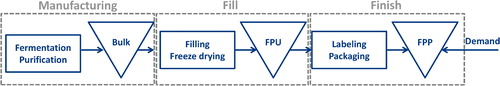
Figure 1 provides a high-level overview of production steps in biomanufacturing. First, biopharmaceuticals are manufactured through a series of fermentation and purification operations. This often results in active pharmaceutical ingredients or antigens, depending on the specific application context. During manufacturing, most of the large scale industry applications use big vessels such as 1000 liter bioreactors. Therefore, the resulting product is called bulk material, and is stored in large quantities for further processing. Next, the bulk material is filled into smaller vials or other forms of packaging during fill-operations. This step typically consists of filling the bulk material into vials and capping them. However, most biopharmaceuticals contain live active ingredients (e.g., antigens), and hence vials often need to be freeze dried. Freeze-drying removes all the liquid from the filled product, such that only a so called “cookie” remains in the vial. Freeze-drying helps to maintain product stability and quality, especially during storage and shipment. The resulting product is called Finished Product Unpacked (FPU). Then, the process continues with finish-operations, where FPUs are labelled and packaged along with a leaflet of medical information. The resulting product is called Final Product Packed (FPP), as shown in Figure 1.

Figure 1. High-level process map of biomanufacturing operations.

The scope of this article is fill-and-finish operations, which are among the most commonly outsourced operations in biomanufacturing. As such, it is estimated that up to 74% of biomanufacturers outsource their fill-and-finish operations (Langer, 2016). This is mainly due to the point that biopharmaceutical fill-and-finish operations require specialized handling and expertise to preserve drug quality. In addition, managing fill-and-finish operations can be often challenging in practice due to several factors:

1. Yield uncertainty in fill-operations: Biopharmaceutical fill-operations involve yield uncertainty. In particular, the freeze-drying process involves complex biological and chemical dynamics that might interfere with the inherent stability of these molecules. For example, the biological activity might not be preserved during freeze-drying, dirt or liquid could remain in the vial after freeze-drying, vials might break during the process, etc. In contrast, finish-operations correspond to labeling and packaging of vials, in which the state-of-the-art technologies often provide reliable production yields.

2. Capacity limitations: As part of regulations, fill-and-finish operations need to comply with predetermined restrictions on the number of vials that can be processed at a time.

3. High holding and shortage costs: Storing and handling of biopharmaceuticals require expensive resources in terms of labor, space and environmental conditions (e.g., cold storage). Furthermore, failure to meet the demand can have critical implications in terms of the cost of disappointing clients and its impact on future orders.

4. Random and non-stationary demand: Demand in the biopharmaceutical industry is often random and non-stationary in the biopharmaceutical industry, i.e., the probability distribution of the demand changes over time as a consequence of the complex dynamics of the biopharmaceutical market. Subsequently, this leads to limitations in forecasts. For example, most biopharmaceutical companies often consider a planning horizon of 1 or 2 years, and forecasting longer periods is often challenging, due to the dynamic and non-stationary nature of the market.

A possible approach to address these challenges is to adjust the production plans frequently. However, this might cause instability in planning. To ensure stability, most biomanufacturers choose to freeze their production decisions for a limited period of time (e.g., 2 months). This implies that the production decisions are made upfront, and do not change in response to the system dynamics during the freeze period. In practice, using freeze periods provides significant visibility in terms of planning and manufacturing, but comes at a price of reduced flexibility. For example, the biomanufacturer cannot respond to yield and demand uncertainty during the freeze period. Therefore, using freeze periods leads to a complex trade-off between reduced flexibility and improved planning stability, and hence adds another layer of challenge in practice.

To address these challenges, we develop a finite-horizon, discounted-cost Markov decision model, and answer the following research questions: How can biomanufacturers manage challenges related to yield uncertainty and freeze periods in biopharmaceutical fill-and-finish operations? What are the optimal production and inventory decisions for fill-and-finish operations? Can we generate guidelines that are easy to implement in practice and yet deliver optimal policies? How can we model and analyze the impact of freeze periods on the expected total cost in this setting? What is the additional cost of freezing production schedules, and how does this cost change with the length of freeze periods? By answering these questions using an optimization framework, we believe that biomanufacturers can significantly reduce costs in fill-and-finish operations.

This work provides several contributions to theory and practice: We analyze the structural characteristics of optimal policies, and propose a zone-based decision-making approach for biopharmaceutical fill-and-finish operations. More specifically, we show that the state space can be partitioned into distinct decision zones that provide rule-of-thumb options for optimal production decisions. These decision zones do not require any restrictive conditions on system parameters, and provide managerial insights that are easy to implement in practice. To the best of our knowledge, this is one of the first studies that builds a stochastic optimization model to address challenges related to yield uncertainty, demand non-stationarity and freeze periods in biopharmaceutical fill-and-finish operations. In addition, the model provides a rigorous basis for communicating mid-term planning challenges within a company, and yields insights related to the cost of using freeze periods in production planning. We also provide an industry case study to illustrate the use of the optimization model.

This research has been conducted in close collaboration with Merck Sharp & Dohme Animal Health (MSD AH) in Boxmeer, Netherlands. MSD AH is one of the top pharmaceutical companies in animal health. Their facility in Boxmeer is a large biomanufacturing center that supplies a wide range of vaccines, anti-infective and anti-parasitic drugs. The research outcomes have also been shared with a larger biomanufacturing community through working group sessions (Nederlandse Biotechnologische Vereniging, 2018). Industry feedback indicates that most biomanufacturers rely on expert opinion and material resource planning calculations that have limited ability to incorporate the manufacturing challenges into decision-making. Therefore, these is a strong need for a rigorous decision-making framework in biopharmaceutical fill-and-finish operations.

The remainder of this article is organized as follows. Relevant literature is reviewed in Section 2. The model is presented in Section 3, and structural results are characterized in Section 4. Freeze periods are modelled in Section 5. An industry case study is presented in Section 6, and concluding remarks are provided in Section 7.

2. Relevant literature

We categorize the relevant literature into two groups: (i) inventory optimization under random yield, and (ii) modelling and analysis of biopharmaceutical fill-and-finish operations.

The literature on random yield has a rich background. We focus on papers that are directly related to our research, and refer the reader to Yano and Lee (1995) for a comprehensive review on random yield models in inventory management. Relevant studies on random yield can be divided into two subcategories: single-period and multi-period models. Karlin (1958) was the first to model a single-period inventory model with random yield and stochastic demand. Among many others, this was followed by Noori and Keller (1986) and Ehrhardt and Taube (1987) who derived an analytical expression for the optimal order quantity when demand was uniformly or exponentially distributed. These results were generalized in Henig and Gerchak (1990) by showing that the optimal order quantity was decreasing in the amount of inventory, and was greater than, or equal to the difference between the critical order point and the current inventory amount. These results have also been extended to single-period, multi-station settings with yield uncertainty (Hwang and Singh (1998), Kogan and Lou (2003), Papachristos and Katsaros (2008)). To improve computational challenges, several heuristics have been developed to optimize inventory decisions (Bollopragada and Morton (1999), Inderfurth (2004), Rekik et al. (2007), Käki et al. (2015)).

Existing literature on multi-period models with random yield often focuses on single-station systems. For example, Mazzola et al. (1987) studied a multi-period problem where demand is deterministic and the yield rate follows a discrete distribution. The authors used dynamic programming to optimally solve the problem when the yield rate is assumed to follow a binomial distribution. In Henig and Gerchak (1990), a multi-period setting is also modeled as a dynamic programming problem under stochastic proportional yields. The authors showed that it is optimal to order when the inventory amout is below a certain critical order point. From this finding, Yano and Lee (1995) derived that it can be beneficial to produce further ahead in the random yield case compared with problems without random yield. Note that the aforementioned studies focus on single-station systems. However, our problem context involves a multi-period, multi-station setting with random yield. Relatively less research has been carried out for such systems, as their analysis is acknowledged as a complex problem (Schmitt and Snyder (2012)). According to Hwang and Singh (1998), such settings are unlikely to produce structurally simple policies. This is also underlined in Tang (1990), where the author approximated the production quantities with a simple rule. A robust optimization model was developed by Zanjani Ait-kadi and Nourelfath, (2010) to manage a real world multi-period, multi-station problem facing yield uncertainty. The authors investigated service levels, and compared the results obtained from the robust optimization model with a stochastic programming model. Similarly, Zanjani Nourelfath and Ait-kadi (2010) developed a multi-stage stochastic programming problem, and combined the information on yield and demand uncertainty into a hybrid decision tree used in the stochastic program.

Our work is closely related to studies on multi-period, multi-echelon inventory systems. When there is no capacity restrictions, it is well known that the optimal policy is an echelon order-up-to policy (Clark and Scarf, 1960). However, when capacity constraints are present, then the structure of the optimal policy is not known in general. Parker and Kapuscinski (2004) and Janakiraman and Muckstadt (2009) derived the optimal policy structure for such systems, but under the assumption that the capacity limits at all stages are identical. Huh and Janakiraman (2010) relaxed this assumption and showed the monotonicity of the optimal policy. However, none of the studies above consider uncertainty in inventory supply. We contribute to this stream of research by analyzing a capacitated system with random production yield. More specifically, our structural analysis of the optimal policy in the fill-and-finish operations extends the work of Huh and Janakiraman (2010) when the most upstream station (namely, the fill station in our setting) also has a capacity restriction and random production yield. In the context of multi-period production planning with random yield, Han et al. (2012) developed a stochastic dynamic program to optimize the finite-horizon expected profit in a two-stage make-to-stock system. Different from Han et al. (2012), we focus on a system with production capacity and provide a structural analysis of the optimal policy.

A vast majority of studies on fill-and-finish operations focus on analyzing the manufacturing and planning challenges encountered in practice. For example, Patro et al. (2002) provided a detailed discussion on factors that lead to random yield in fill-finish, and reviewed the critical process parameters and configurations to maintain drug safety and efficacy during fill-finish. Several studies overview the current trends and challenges in biopharmaceutical fill-finish, especially in freeze-drying process (McLeod et al. (2011), Rios (2012), Scott and Rios (2015), Gutka and Prasad (2015)). On the other hand, there are only a few studies that model the risks and uncertainties in fill-and-finish operations. In this context, we observe that existing studies largely focus on simulation modeling and statistical analysis of biomanufacturing operations. For example, Petrides et al. (2011) developed a simulation model for fill-finish facilities, and used a scheduling tool to reduce cycle times and costs. Khairuddin et al. (2016) developed a simulation model to evaluate layout design options at a fill-finish facility. Jiang et al. (2011) used statistical regression to help decision makers with estimating and optimizing viscosity and filter capacity during fill-finish. A case study on quality risk management during fill-finish was described by Miller (2009). Simulation models have also been used to assess capacity in biomanufacturing (Robinson et al. (2017)). However, existing simulation studies are not equipped to answer the research questions defined in Section 1, especially to those related to determining optimal policies.

3. Model formulation

We develop a discrete-time, finite-horizon, discounted-cost Markov decision model to optimize production decisions in biopharmaceutical fill-and-finish operations. First, we describe the notation used to build the model.

Decision epochs: We consider a discrete-time problem where the planning horizon is equally divided into T decision epochs, such that $\mathcal{T}=\{t:0,1,\dots ,T-1\}$ represents the set of all decision epochs. Time between two decision epochs is referred to as a period; i.e., the tth decision epoch represents the beginning of period t + 1. In our problem setting in practice, each period typically corresponds to a month, and the planning horizon is often 1 to 2 years.

States: Let i = 1, 2 represent the production station for fill- and finish-operations, respectively. The state space is defined as $\mathcal{S}\equiv {\mathcal{S}}_1\times {\mathcal{S}}_2$ where ${\mathcal{S}}_1\in {\mathbb{R}}_{+}$ and ${\mathcal{S}}_2\in \mathbb{R}.$ The state $s_{i,t}\in {\mathcal{S}}_i$ represents the inventory level at production station $i\in \{1,2\}$ and decision epoch $t\in \mathcal{T}.$ We let $s_{1,t}\ge 0$ as a system requirement to generate feasible production plans. Note that $s_{2,t}$ can be negative to indicate the amount of backlog in the finish-operations at decision epoch t. Raw material for fill-operations is assumed to be ample. This aligns with current practice where raw materials are available in large vessels at bulk quantities.

Actions: The action space is defined as $\mathcal{U}\equiv {\mathcal{U}}_1\times {\mathcal{U}}_2.$ The action $u_{i,t}\in {\mathcal{U}}_i$ represents the number of vials to be produced in production station $i\in \{1,2\}$ at decision epoch $t\in \mathcal{T}.$ Due to regulatory requirements, the biomanufacturer needs to comply with a predetermined batch size b_i at production station i. In addition, each production station has a limited capacity during a period. Therefore, the inclusion of limited capacity and fixed batch size truncates the action space to ${\mathcal{U}}_i=\{u_{i,t}:0,b_i,2b_i,3b_i,\dots ,m_i{b}_i\}$ for i = 1, 2 at $t\in \mathcal{T},$ where the parameter $m_i{b}_i$ denotes the maximum number of vials that can be processed at production station i during a period. For convenience, the structural analysis in Section 4 assumes continuous batch sizing with $u_{i,t}\in [0,m_i{b}_i].$ Note that the amount of work-in-progress inventory in the fill-operations constrains the production quantity at the finish-operations, i.e., $s_{1,t}\ge u_{2,t}$ at $t\in \mathcal{T}.$

State transitions: To determine the state transition probabilities, we first focus on the random and often non-stationary demand for biopharmaceutical drugs. Let the non-negative random variable D_t represent the demand in period t with probability density function $g_t(·)$ and realization d_t, $t\in \{1,\dots ,T\}.$ Note that $g_t(·)$ is a function of t due to demand non-stationarity. Next, we focus on modeling the yield uncertainty in fill-operations. The amount obtained at fill is a random fraction R of the planned production quantity $u_{1,t}$ at $t\in \mathcal{T}.$ The random fraction R has probability distribution $f(·)$ with realization r on the interval $[0,1].$ Therefore, the future state $(s_{1,t+1},s_{2,t+1})$ at $t+1\in \mathcal{T}$ is determined by the current state $(s_{1,t},s_{2,t}),$ action $(u_{1,t},u_{2,t}),$ realization of the yield fraction (r), and demand realization d_t at $t\in \mathcal{T},$ i.e., (1) $$s_{i,t+1}=\{\begin{array}{cc}{s}_{1,t}-u_{2,t}+(u_{1,t}\times r)\hfill & \text{for} i=1,\hfill \\ s_{2,t}-d_t+u_{2,t}\hfill & \text{for} i=2.\hfill \end{array}$$(1)

It follows from Equation (1)(1) $$s_{i,t+1}=\{\begin{array}{cc}{s}_{1,t}-u_{2,t}+(u_{1,t}\times r)\hfill & \text{for} i=1,\hfill \\ s_{2,t}-d_t+u_{2,t}\hfill & \text{for} i=2.\hfill \end{array}$$(1) that the demand d_t is observed at finish-operations (i = 2), and work-in-progress inventory is pulled from fill-operations (i = 1) based on the production amount $u_{2,t}$ at the finish-operations. Equation (1)(1) $$s_{i,t+1}=\{\begin{array}{cc}{s}_{1,t}-u_{2,t}+(u_{1,t}\times r)\hfill & \text{for} i=1,\hfill \\ s_{2,t}-d_t+u_{2,t}\hfill & \text{for} i=2.\hfill \end{array}$$(1) indicates that the production amount $u_{i,t}$ is available at the beginning of decision epoch t + 1. In addition, we note that Equation (1)(1) $$s_{i,t+1}=\{\begin{array}{cc}{s}_{1,t}-u_{2,t}+(u_{1,t}\times r)\hfill & \text{for} i=1,\hfill \\ s_{2,t}-d_t+u_{2,t}\hfill & \text{for} i=2.\hfill \end{array}$$(1) assumes a proportional random yield model, which was validated using 2 years of production data (i.e., the data provided a normalized ratio of the total amount of yield obtained from the freeze-drying process to the total amount of input that goes into the freeze-drying process). In compliance with standard industry practice, we focus on the modeling and analysis of yield uncertainty in fill-operations. Nevertheless, our model formulation is flexible to capture yield uncertainty in finish-operations, and would result in similar insights.

Costs: Costs depend on the state $(s_{1,t},s_{2,t})$ at decision epoch $t\in \mathcal{T}.$ When inventory is held, cost h_i is incurred per unit of inventory at production station i. A penalty cost of shortage, p₂, has to be paid for each unit short in finish-operations. This leads to incurring the cost (2) $$c(s_{1,t},s_{2,t})=(h_1\times s_{1,t})+(h_2\times {\left[s_{2,t}\right]}^{+}+p_2\times {[-s_{2,t}]}^{+}),$$(2) in period t, where ${[z]}^{+}=\max \{0,z\}.$

The value function: At the end of the planning horizon t = T, the terminal value is (3) $$V_T(s_{1,T},s_{2,T})=c(s_{1,T},s_{2,T}),$$(3) and the value function $V_t(s_{1,t},s_{2,t})$ for all $t\in \{0,1,\dots ,T-1\}$ is (4) $$V_t(s_{1,t},s_{2,t})=\underset{(u_{1,t},u_{2,t})\in \mathcal{U}}{\min }\{c(s_{1,t},s_{2,t})+\gamma ·\mathbb{E}[V_{t+1}(S_{1,t+1},S_{2,t+1})|s_{1,t},s_{2,t},u_{1,t},u_{2,t}]\},$$(4) where the expected value $\mathbb{E}[V_{t+1}(S_{1,t+1},S_{2,t+1})|s_{1,t},s_{2,t},u_{1,t},u_{2,t}]$ is given by (5) $$\begin{array}{c}\mathbb{E}[V_{t+1}(S_{1,t+1},S_{2,t+1})|s_{1,t},s_{2,t},u_{1,t},u_{2,t}]\hfill \\ \hspace{1em}={\int }_{r=0}^1{\int }_{d_t=0}^{\infty }{V}_{t+1}(s_{1,t}-u_{2,t}+u_{1,t}\times r_1,s_{2,t}-d_t+u_{2,t})\times f(r)\times g_t(d_t) \mathsf{d}{d}_t \mathsf{d}r.\hfill \end{array}$$(5)

The parameter γ indicates the discount factor such that $0\le \gamma \le 1.$ In Equations (3)(3) $$V_T(s_{1,T},s_{2,T})=c(s_{1,T},s_{2,T}),$$(3) and (4)(4) $$V_t(s_{1,t},s_{2,t})=\underset{(u_{1,t},u_{2,t})\in \mathcal{U}}{\min }\{c(s_{1,t},s_{2,t})+\gamma ·\mathbb{E}[V_{t+1}(S_{1,t+1},S_{2,t+1})|s_{1,t},s_{2,t},u_{1,t},u_{2,t}]\},$$(4) , the objective is to minimize the total discounted cost by optimizing the production decisions $(u_{1,t},u_{2,t})\in \mathcal{U}.$ Then, $V_t(s_{1,t},s_{2,t})$ expresses the minimum total discounted cost over the periods $t,t+1,\dots ,T$ given that the state at time t is $(s_{1,t},s_{2,t}).$ Note that the expectation in Equation (5)(5) $$\begin{array}{c}\mathbb{E}[V_{t+1}(S_{1,t+1},S_{2,t+1})|s_{1,t},s_{2,t},u_{1,t},u_{2,t}]\hfill \\ \hspace{1em}={\int }_{r=0}^1{\int }_{d_t=0}^{\infty }{V}_{t+1}(s_{1,t}-u_{2,t}+u_{1,t}\times r_1,s_{2,t}-d_t+u_{2,t})\times f(r)\times g_t(d_t) \mathsf{d}{d}_t \mathsf{d}r.\hfill \end{array}$$(5) is taken with respect to the probability distribution of the uncertain yield $f(·)$ and the time-dependent demand $g_t(·).$ We let $u_{i,t}^{*}(s_{1,t},s_{2,t})$ denote an optimal production amount at production station i when the system state is $(s_{1,t},s_{2,t})$ at time $t\in \mathcal{T},$ and ${\pi }_t^{*}$ denote an optimal policy (i.e., function that maps a system state into an optimal action) at time t until the end of planning horizon T. Hereinafter, we call the model presented in this section the base model.

The base model is developed as a finite-horizon model for multiple reasons. First, in practice, biopharmaceutical companies often optimize their operations by considering the foreseeable future, and set their business strategies for a fixed planning horizon accordingly. For example, at MSD AH, production planners consider a planning window of typically 1 year but no longer than 2 years. This is mainly because of the uncertainties in the market (e.g., more effective drugs can enter the market, and product lines, as well as production processes, evolve over time). Second, products that we consider at MSD AH have nonstationary demand, for which forecasts are available only for the next 12 to 24 months. At MSD AH, sales organizations generate such forecasts to serve as direct input to our finite-horizon model (in Section 5, we present an approach that relies on solving the long-run business problem by using our base model through a rolling-horizon mechanism over time). Furthermore, at MSD AH, the Material Resource Planning (MRP) activities are conducted every month based on a finite planning horizon of 1 or 2 years. The decisions considered in this article are mid-term planning decisions that are part of such MRP activities. Finally, in principle, a finite-horizon model can approximate an infinite-horizon model given that the number of decision epochs is sufficiently large.

4. Structural analysis

We start our analysis by summarizing and developing some preliminary technical results in Section 4.1. Then, we analyze the structural properties of optimal policies for the fill-operations and finish-operations in Sections 4.2 and 4.3, respectively. All proofs are available in the Appendix.

4.1. Preliminaries

Our analysis relies on the notion of $L^{♮}$-convexity (see, e.g., Simchi-Levi et al., 2014). To be able to define $L^{♮}$-convexity, we first introduce the concept of submodularity. Let $\mathcal{V}\subseteq {\mathbb{R}}^n$ be a polyhedron that forms a lattice (i.e., for any x, $\mathbf{x}\prime \in \mathcal{V},$ it is known that $\mathbf{x}\wedge \mathbf{x}\prime ,\mathbf{x}\vee \mathbf{x}\prime \in \mathcal{V},$ where $\wedge$ and $\vee$ are component-wise minimum and component-wise maximum operators, respectively). A function $f:\mathcal{V}\to \mathbb{R}$ is submodular on the set $\mathcal{V}$ if, for any x, $\mathbf{x}\prime \in \mathcal{V},$ the inequality $f(\mathbf{x})+f(\mathbf{x}\prime )\ge f(\mathbf{x}\wedge \mathbf{x}\prime )+f(\mathbf{x}\vee \mathbf{x}\prime )$ holds. For a twice-differentiable f, it follows that f is submodular if and only if ${\partial }^{2}f(\mathbf{x})/\partial x_i\partial x_j\le 0$ for any distinct indexes i and j and for any $\mathbf{x}\in \mathcal{V}.$

Following Zipkin (2008), we say that the function $f:\mathcal{V}\to \mathbb{R}$ is $L^{♮}$-convex if the function $\psi (\mathbf{v},\xi )=f(\mathbf{v}-\xi \mathbf{e})$ is submodular on $\mathcal{V}\times {\mathbb{R}}_{-}$ where $\mathbf{v}\in \mathcal{V},$ e is the n-dimensional all-ones vector, and $\xi \le 0.$ $L^{♮}$-convexity of a function implies that the function has the convexity, submodularity, and diagonal-dominance properties (Gong and Chao, 2013), which are desirable properties for the analysis of optimal policy structures.

Next, we extend Lemma 1 in Zipkin (2008) and introduce a property of $L^{♮}$-convexity that will be useful for our analysis under random yield in fill-operations.

Lemma 1.

Suppose that $f:\mathcal{V}\stackrel{}{\to }\mathbb{R}$ is an $L^{♮}$-convex function and $r\ge 0$. In this case, the function $g:\mathcal{V}\times {\mathbb{R}}_{-}\to \mathbb{R}$, which is defined as $g(\mathbf{v},\xi )=f(\mathbf{v}-\xi r\mathbf{e})$, is also $L^{♮}$-convex.

Similar to Zipkin (2008) and Huh and Janakiraman (2010), the core of our analysis includes a transformation of the state variables of the Markov decision process model. To be specific, our objective is to obtain $L^{♮}$-convex value functions after transformation and exploit the properties of $L^{♮}$-convexity in our analysis, although the value functions (i.e., Equations (3)(3) $$V_T(s_{1,T},s_{2,T})=c(s_{1,T},s_{2,T}),$$(3) and (4)(4) $$V_t(s_{1,t},s_{2,t})=\underset{(u_{1,t},u_{2,t})\in \mathcal{U}}{\min }\{c(s_{1,t},s_{2,t})+\gamma ·\mathbb{E}[V_{t+1}(S_{1,t+1},S_{2,t+1})|s_{1,t},s_{2,t},u_{1,t},u_{2,t}]\},$$(4) ) are not $L^{♮}$-convex in the original state variables. Intuitively, the role of state transformation is to ensure that the state variables have complementary relationships, and hence, the $L^{♮}$-convexity of the value functions is preserved under minimization (see Topkis (1998) for details on complementarity and Li and Yu (2014) for its role in the structural analysis of dynamic inventory problems).

4.2. Fill operations

For notational convenience, we drop the subscript t from the state and action variables when possible in the remainder of the analysis. Let w₁ = s₁ and $w_2=s_1+s_2.$ Notice that the transformed state variables $(w_1,w_2)\in \mathbb{R}\times \mathbb{R},$ and the corresponding state space is a lattice. Let $u_j\ge 0$ denote the production decision of production station $j\in \{1,2\};$ i.e., u₁ and u₂ are the number of vials produced in the fill-operations and finish-operations, respectively. Let ${\overline{w}}_1=w_1-u_2$ and $\xi =-u_1.$ For $t\in \mathcal{T},$ the value functions for the transformed problem can be written as (6) $$J_t(w_1,w_2)=c(w_1,w_2-w_1)+\gamma f_{t+1}(w_1,w_2),$$(6) where (7) $$\begin{array}{c}{f}_{t+1}(w_1,w_2)=\underset{\xi ,{\overline{w}}_1}{\text{min}}\mathbb{E}\left[J_{t+1}({\overline{w}}_1-\xi R,w_2-\xi R-D_t)\right],\\ \mathrm{s}.\mathrm{t}.-m_1{b}_1\le \xi \le 0,\\ -m_2{b}_2\le {\overline{w}}_1-w_1\le 0,\\ 0\le {\overline{w}}_1.\end{array}$$(7) with the terminal value function given by $J_T(w_1,w_2)=c(w_1,w_2-w_1).$

In Theorem 1(i), we show that the value function in each period is an $L^{♮}$-convex function after the transformation of the state variables. This will enable us to show in Theorem 1(ii) that the optimal policy in the fill-operations is a monotone function of the inventory levels in the fill and finish operations.

Theorem 1.

(i) The value functions $J_t(w_1,w_2)$ are $L^{♮}$-convex in w₁ and w₂ for $t=1,2,\dots ,T$. (ii) The optimal number of vials produced in the fill-operations $u_{1,t}^{*}(s_1,s_2)$ is nonincreasing in s₁ and $s_2$ for $t\in \mathcal{T}.$

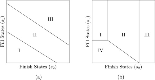
It immediately follows from Theorem 1(ii) that the state space can be partitioned into decision zones for fill-operations, as summarized in Corollary 1.

Corollary 1

(Decision zones for Fill). At time $t\in \mathcal{T}$, optimal policy for fill-operations has the following characteristics:

1. If $u_{1,t}^{*}({\widehat{s}}_1,{\widehat{s}}_2)=m_1{b}_1$ for $({\widehat{s}}_1,{\widehat{s}}_2)\in \mathcal{S}$, then $u_{1,t}^{*}(s_1,s_2)=m_1{b}_1$ for any $(s_1,s_2)$ with $s_1\le {\widehat{s}}_1$ and $s_2\le {\widehat{s}}_2.$

2. If $u_{1,t}^{*}({\check{s}}_1,{\check{s}}_2)=0$ for $({\check{s}}_1,{\check{s}}_2)\in \mathcal{S}$, then $u_{1,t}^{*}(s_1,s_2)=0$ for any $(s_1,s_2)$ with $s_1\ge {\check{s}}_1$ and $s_2\ge {\check{s}}_2.$

Consequently, it follows that optimal decisions for fill-operations can be divided into Zones I, II, III, where Zone I includes all states $(s_1,s_2)\in \mathcal{S}$ in which $u_{1,t}^{*}(s_1,s_2)=m_1{b}_1,$ Zone II in which $0<u_{1,t}^{*}(s_1,s_2)<m_1{b}_1,$ and Zone III in which $u_{1,t}^{*}(s_1,s_2)=0.$ For practitioners, these decision zones provide important managerial insights on optimal policies, and are easy to implement in practice. For example, if the state of the system is an element of Zone I at time t, then optimal policy for the fill-operations requires to produce at maximum capacity. In contrast, when the system state belongs to Zone III, then it is optimal to not produce anything in the fill-operations. In the case where the system state is within Zone II, then optimal policy for fill-operations has a control-limit-type structure, and these control-limits are nonincreasing in the inventory levels in each production station. A visual representation of the decision zones is provided in Figure 2. For simplicity, zones in Figure 2 are separated with straight lines, however, we note that these lines can be curvy (in the form of a more general switching curves) and the zones may have a variety of forms in theory.

Figure 2. An illustration of possible decision zones for (a) fill and (b) finish operations.

4.3. Finish operations

In this section, the objective is to study the monotonicity of optimal production decisions in the finish-operations. Recall that the intuition behind the state transformation in Section 4.2 was to make sure that the state in the next decision epoch has a special form, where a term proportional to ξ (i.e., the decision of the fill station) is subtracted from each state component; see the objective function in Equation (7)(7) $$\begin{array}{c}{f}_{t+1}(w_1,w_2)=\underset{\xi ,{\overline{w}}_1}{\text{min}}\mathbb{E}\left[J_{t+1}({\overline{w}}_1-\xi R,w_2-\xi R-D_t)\right],\\ \mathrm{s}.\mathrm{t}.-m_1{b}_1\le \xi \le 0,\\ -m_2{b}_2\le {\overline{w}}_1-w_1\le 0,\\ 0\le {\overline{w}}_1.\end{array}$$(7) . In this way, $L^{♮}$-convexity is preserved after the minimization. However, the same state transformation does not lead to the preservation of $L^{♮}$-convexity when the finish decision is considered. Therefore, in this section, we adopt an alternative transformation of the state variables based on Huh and Janakiraman (2010). Different from Section 4.2, we now let $w_1=-s_1$ and w₂ = s₂. Notice that $(w_1,w_2)\in {\mathbb{R}}_{-}\times \mathbb{R},$ and the corresponding state space is a lattice. Furthermore, we now let ${\overline{w}}_1=w_1-u_1$ and $\xi =-u_2.$ For $t\in \mathcal{T},$ the value functions for the transformed problem can be written as (8) $$J_t(w_1,w_2)=c(-w_1,w_2)+\gamma f_{t+1}(w_1,w_2),$$(8) where (9) $$\begin{array}{c}{f}_{t+1}(w_1,w_2)=\underset{\xi ,{\overline{w}}_1}{\text{min}}\mathbb{E}\left[J_{t+1}(R{\overline{w}}_1+(1-R)w_1-\xi ,w_2-\xi -D_t)\right],\\ \mathrm{s}.\mathrm{t}.-m_2{b}_2\le \xi \le 0,\\ w_1-\xi \le 0,\\ w_1-{\overline{w}}_1\le m_1{b}_1.\end{array}$$(9) with the terminal value function given by $J_T(w_1,w_2)=c(-w_1,w_2).$ For a general distribution for the yield random variable R, the value function $J_t(w_1,w_2)$ in Equation (8)(8) $$J_t(w_1,w_2)=c(-w_1,w_2)+\gamma f_{t+1}(w_1,w_2),$$(8) is not necessarily $L^{♮}$-convex in w₁ and w₂. This is because the $L^{♮}$-convexity of the function $J_{t+1}(w_1,w_2)$ in w₁ and w₂ does not guarantee the $L^{♮}$-convexity of the function $J_{t+1}(r{\overline{w}}_1+(1-r)w_1-\xi ,w_2-\xi -d_t)$ in w₁, ${\overline{w}}_1,$ w₂ and ξ for $r\in (0,1),$ where r and d_t denote the realizations of the random variables R and D_t, respectively. Therefore, the objective function in Equation (9)(9) $$\begin{array}{c}{f}_{t+1}(w_1,w_2)=\underset{\xi ,{\overline{w}}_1}{\text{min}}\mathbb{E}\left[J_{t+1}(R{\overline{w}}_1+(1-R)w_1-\xi ,w_2-\xi -D_t)\right],\\ \mathrm{s}.\mathrm{t}.-m_2{b}_2\le \xi \le 0,\\ w_1-\xi \le 0,\\ w_1-{\overline{w}}_1\le m_1{b}_1.\end{array}$$(9) is not necessarily $L^{♮}$-convex in ${\overline{w}}_1,$ w₁, w₂ and ξ. Thus, different from Section 4.2, the $L^{♮}$-convexity of the function $f_{t+1}(w_1,w_2)$ and subsequently the $L^{♮}$-convexity of the value function $J_t(w_1,w_2)$ in Equation (8)(8) $$J_t(w_1,w_2)=c(-w_1,w_2)+\gamma f_{t+1}(w_1,w_2),$$(8) do not necessarily hold for a general distribution for the yield random variable R. In Theorem 2(i), we show that the value function $J_t(w_1,w_2)$ is $L^{♮}$-convex for the following special types of production yield in the fill-operations: (i) Deterministic yield: R = r with probability 1; (ii) All-or-nothing yield: R = 1 with probability r and R = 0 with probability $1-r.$ All-or-nothing type of yield is especially relevant in biomanufacturing due to random shocks that can affect the entire production (see, e.g., Tomlin (2009), Martagan et al. (2016)). For example, during the freeze-drying process, physico-chemical process parameters (i.e., temperature, moisture, pH, etc.) might deviate from their pre-specified control ranges due to bacterial contamination, human errors or equipment failure. In such cases, the whole batch needs to be scrapped to comply with regulatory requirements.

Theorem 2.

Suppose that the production yield in fill-operations is deterministic or has all-or-nothing type of yield uncertainty. (i) The value functions $J_t(w_1,w_2)$ is $L^{♮}$-convex in w₁ and w₂ for $t=1,2,\dots ,T$. (ii) The optimal number of vials produced in the finish-operations $u_{2,t}^{*}(s_1,s_2)$ is nondecreasing in s₁ and nonincreasing in $s_2$ for $t=1,2,\dots ,T-1.$

The monotonicity of optimal policies in finish-operations, as described in Theorem 2, leads to specific decision zones for the finish station (when the production yield in fill-operations is deterministic or has all-or-nothing type of uncertainty). This is summarized in Corollary 2.

Corollary 2

(Decision zones for Finish). At time $t\in \mathcal{T}$, optimal policy for finish-operations has the following characteristics:

1. If $u_{2,t}^{*}({\widehat{s}}_1,{\widehat{s}}_2)=m_2{b}_2$ for $({\widehat{s}}_1,{\widehat{s}}_2)\in \mathcal{S}$, then $u_{2,t}^{*}(s_1,s_2)=m_2{b}_2$ for any $(s_1,s_2)$ with $s_1\ge {\widehat{s}}_1$ and $s_2\le {\widehat{s}}_2.$

2. If $u_{2,t}^{*}({\check{s}}_1,{\check{s}}_2)=0$ for $({\check{s}}_1,{\check{s}}_2)\in \mathcal{S}$, then $u_{2,t}^{*}(s_1,s_2)=0$ for any $(s_1,s_2)$ with $s_1\le {\check{s}}_1$ and $s_2\ge {\check{s}}_2.$

3. If $u_{2,t}^{*}({\overline{s}}_1,{\overline{s}}_2)={\overline{s}}_1$ for $({\overline{s}}_1,{\overline{s}}_2)\in \mathcal{S}$, then $u_{2,t}^{*}({\overline{s}}_1,s_2)={\overline{s}}_1$ for any $({\overline{s}}_1,s_2)$ with $s_2\le {\overline{s}}_2.$

It is important to note that we prove the monotonicity of the optimal policy in fill-operations (Theorem 1) under any general probability distribution for the yield in the fill station. On the other hand, we are able to analytically prove the monotonicity of the optimal policy in finish-operations only when the yield in the fill station is deterministic or has all-or-nothing type of uncertainty. Nevertheless, in our case study with industry data in Section 6, we observe that the monotonicity of optimal policies in the finish station continues to hold (under uniformly distributed yield random variable and a finite action space). In our additional numerical experiments with right-skewed, left-skewed and symmetric density functions for the yield random variable, we continue to observe that the optimal production quantity at the finish station still shows monotonicity. In such cases, the decisions for finish-operations can be divided into four zones, where Zone I includes all states $(s_1,s_2)\in \mathcal{S}$ in which $u_{2,t}^{*}(s_1,s_2)=m_2{b}_2$ (i.e., produce at maximum finish capacity), Zone III in which $u_{2,t}^{*}(s_1,s_2)=0$ (i.e., do nothing), Zone IV in which $u_{2,t}^{*}(s_1,s_2)=s_1$ (i.e., produce at maximum fill inventory capacity), and Zone II as the remaining states. Figure 2(b) illustrates a possible layout of the decision zones in finish-operations.

The zone-based decision-making presented in our work provides a new, rigorous approach for decision-making in biopharmaceutical fill-and-finish operations. From a practical point of view, these decision zones are easy to adopt and implement in current practice. The case study presented in Section 6 uses industry data from MSD AH to illustrate how these decision zones can be generated and used in practice.

5. Planning with freeze periods

We expand the base model presented in Section 3 to incorporate freeze periods into production plans. First, we describe how MSD AH works with freeze periods in practice, and then introduce a formal description of the model to incorporate freeze periods into decision-making.

5.1. Current practice

There are several different ways of freezing the production plans in practice. In this article, we focus on the current practice at MSD AH, where production planners conduct a planning activity at the beginning of every period in order to generate a production plan for the next T periods. The length T of a planning horizon is often 1 or 2 years, due to the highly dynamic and non-stationary nature of the biopharmaceutical market. The length of a period is typically a month, as the periodic planning activities are part of monthly aggregate planning activities (i.e., in compliance with MRP activities).

Every time a planning activity is conducted, it generates a production plan for the upcoming T periods. Once a production plan is generated, the plan for the first L periods is communicated to the manufacturing team, and cannot be further changed. Thus, this is referred to as a freeze period. In Figure 3, we illustrate this mechanism for a planning horizon of T = 12 months and a freeze period of length L = 2 months. In this example, the first planning activity is conducted at the beginning of January 2019, and generates a monthly production plan until the end of December 2019. In this production plan, the first 2 months (January and February) are frozen, as represented with dashed boxes in Figure 3. The next planning activity is conducted at the beginning of February 2019 and generates a monthly production plan until the end of January 2020. However, this production plan assumes that the production decisions of February 2019 are fixed (because it was part of the freeze period at the previous planning activity). That is, the frozen decisions are carried forward to the next planning activities. At each planning activity, the company works with the most recent demand forecasts for the next T periods to determine the production plans that minimize the total expected cost in a planning window of T periods. In this sense, the company adopts a rolling-horizon approach, in which the base model is repeatedly solved every period with updated demand forecasts. These forecasts are generated by a separate department in the company, referred as Sales Organizations, specialized on market analysis.

Figure 3. Freeze periods over a rolling horizon.

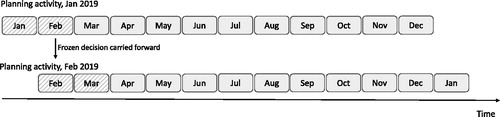
In practice, MSD AH typically uses a freeze period of length L = 2 months, as illustrated in Figure 3. The motivation of the company for using freeze periods is to ensure that, at all times, they have full visibility of their production activities in the next L periods. An alternative policy could be to generate a new production plan for the next T periods at every L periods. Although such a policy might potentially perform better, it is not preferred in practice because it does not always provide full visibility on the production activities of the next L periods.

5.2. Modeling of freeze periods

The objective of this section is to formally describe how we model the dynamics of the freeze periods explained in Section 5.1. We let $\omega \in \{1,2,\dots \}$ denote the index of the planning activity, where each planning activity ω generates a production plan for the upcoming T periods. Let L denote the length of the freeze period (also note that $L\le T$). Each planning activity uses the latest available demand forecasts (for the next T periods). We model this by assuming that a collection of the probability distribution functions ${\widehat{g}}_{\omega }\triangleq \{{\widehat{g}}_{t,\omega }(·):t=\omega ,\omega +1,\omega +T-1\}$ is available at the time of the planning activity ω, where ${\widehat{g}}_{t,\omega }(·)$ denotes an estimate of the demand density function $g_t(·)$ available at planning activity w. We consider that demand forecasts are provided exogenously as an input to the model and assume that there is no demand learning mechanism in the model. The pseudo-code in Algorithm 1 outlines how the base model is used in practice in a rolling horizon basis in the presence freeze periods.

Let ${\pi }_{\omega }$ denote the T-period production plan generated by the planning activity ω (${\pi }_{\omega }$ is defined as an arbitrary policy for ω = 1). Algorithm 1 takes ${\pi }_{\omega -1},$ the production plan generated in planning activity $\omega -1,$ as input for the planning activity ω. We let ${\pi }^{*}=({\pi }_0,\dots ,{\pi }_{T-1})$ denote the optimal policy obtained by solving the base model in Section 3 via backward induction for all $t\in \{0,\dots ,T-1\};$ i.e., ${\pi }_t=(u_{1,t}^{*}(s_1,s_2),u_{2,t}^{*}(s_1,s_2))$ for all $(s_1,s_2)\in \mathcal{S}.$ In Step 3 of Algorithm 1, notice that the collection of the demand distributions (for the next T periods) available at planning activity ω is used as input in the base model. We note that both ${\pi }_{\omega }$ and ${\pi }^{*}$ consist of T elements, where each element is a pair of vectors representing a production policy (i.e., a function that maps a system state into a production decision) for the fill and finish operations. Let ${\pi }_{\omega }(i)$ denote the ith element of ${\pi }_{\omega },$ and ${\pi }^{*}(i)$ denote the ith element of ${\pi }^{*}.$ For the first planning activity (i.e., ω = 1), clearly, the solution from the base model is the output (step 6). Otherwise, we note that the output of the ωth planning activity is a T-period production plan, where the first L – 1 elements are the second to Lth elements of the previous production plan ${\pi }_{\omega -1}$ and the remaining $T-L+1$ elements are the ones coming from the solution of the base model under new demand distributions (step 8).

Algorithm 1. Procedure for the planning activity ω with freeze periods

1: Inputs: L, $h_1,h_2,p_2,f(·),{\widehat{g}}_{\omega },$ and ${\pi }_{\omega -1}$

2: Output: ${\pi }_{\omega }$

Require: $L\ge 2$ ⊳ L = 1 implies having no freeze period

3: Set $g_{t-\omega +1}(·)={\widehat{g}}_{t,\omega }(·)$ for $t=\omega ,\omega +1,\dots ,\omega +T-1.$

4: Let ${\pi }^{*}=({\pi }_0,\dots ,{\pi }_{T-1})$ where ${\pi }_t=(u_{1,t}^{*}(s_1,s_2),u_{2,t}^{*}(s_1,s_2))$ for all $(s_1,s_2)\in \mathcal{S}.$

5: if ω = 1 then

6:  ${\pi }_{\omega }={\pi }^{*},$

7: else

8:  ${\pi }_{\omega }=({\pi }_{\omega -1}(2),\dots ,{\pi }_{\omega -1}(L),{\pi }^{*}(L),\dots {\pi }^{*}(T).$

9: end if

6. Numerical analysis: An industry case study

We present a case study from MSD AH in Boxmeer, Netherlands. The case study involves fill-and-finish operations of a specific type of antigen filled and sold in form of vials. Name and characteristics of this antigen are not disclosed to protect confidentiality. First, we introduce the problem setting (Section 6.1), and then analyze the financial implications of yield uncertainty (Section 6.2) and freeze periods (Section 6.3).

6.1. Problem setting

Fill-and-finish operations have a fixed batch size of 0.25 million vials (mln VL). Fill-operations have a maximum production capacity of 6 mln VL per month, and hence this leads to the action space ${\mathcal{U}}_1=\{0,0.25,0.5,\dots ,6\}$ mln VL. Finish-operations have a maximum production capacity of 8 mln VL per month with the action space ${\mathcal{U}}_2=\{0,0.25,0.5,\dots ,8\}$ mln VL. As an operational policy, the company does not store more than 15 mln VL, which sets an upper bound on the state space.

To protect confidentiality, we use representative values for model inputs. Holding cost is $h_1=\$0.5$ per vial in fill-operations, and $h_2=\$0.8$ per vial in finish-operations. Penalty cost of shortage is $p_2=\$6.2$ per vial, and includes the cost of internal planning and scheduling efforts to meet backorders, cost of disappointing clients and its impact on future orders, etc. Statistical analysis of monthly sales data over the last 2 years and forecast information for the upcoming 2 years indicate that monthly demand can be modelled with a normal distribution (see the supplement files for the parameters of demand distribution used in the numerical analysis).

Analysis of two years of production data showed that the random yield fraction was uniformly distributed for fill-operations in the interval $[0.70,0.90].$ Therefore, we obtain the mean $\mathbb{E}[R]=0.80$ and coefficient of variation $CV[R]=0.07.$ In compliance with industry standards, data analysis showed that no significant yield losses were encountered in finish-operations.

In alignment with the current production planning strategy of MSD AH, we consider a planning horizon of T = 24 months, where each decision epoch corresponds to the beginning of a month. In practice, MSD AH’s planning horizon is often 1 or 2 years. This is mainly because the biopharmaceutical market is highly dynamic and non-stationary, and hence it is often challenging to generate reliable policies for a period longer than 1 or 2 years (see Sections 3 and 5.1 for further details). To check the robustness of optimal actions to different lengths of planning horizon, we conducted additional numerical experiments. We concluded that the effect of the length of the planning horizon on optimal production decisions at the beginning of the planning horizon decreases as T approaches 24 months. Nevertheless, the rolling horizon approach presented in Section 5.2 (and numerically evaluated in Section 6.3) enables us to plan for the foreseeable future in practice. All numerical experiments use a discount factor of $\gamma =0.99.$ This problem setting is referred as the base case in our numerical analysis. We solve the problem with backward induction, and use a discretization scheme of the state space based on the minimum allowed batch size. We also tested the sensitivity to finer discretization schemes, and concluded that optimal cost and policies were robust to finer discretization levels.

6.2. Insights on yield uncertainty

The main aim of this section is to help operations managers understand the impact of yield uncertainty on optimal costs and decision zones. For this purpose, we focus on the following characteristics of the yield random variable R: (i) average yield, and (ii) variability in yield. In compliance with industry data, we use uniform distribution for the fraction R, and define the following scenarios: Base case ($\mathbb{E}[R]=0.80$ and $CV[R]=0.07$), no yield loss (deterministic R = 1), lower yield loss ($\mathbb{E}[R]=0.90$ and $CV[R]=0.07$), higher yield loss ($\mathbb{E}[R]=0.70$ and $CV[R]=0.07$), no variability (deterministic R = 0.8), higher variability ($\mathbb{E}[R]=0.80$ and $CV[R]=0.14$), and all-or-nothing yield ($\mathbb{E}[R]=0.80$ and $CV[R]=0.50;$ i.e., R = 1 with probability 0.8 and R = 0 with probability 0.2). These scenarios are defined based on input from practitioners to represent a variety of cases from the industry. The scenarios no yield loss, lower yield loss and higher yield loss enable us to study the impact of average yield, whereas the scenarios no variability, higher variability, and all-or-nothing yield enable us to study the impact of yield variability on operational performance.

6.2.1. Financial implications of yield uncertainty in fill-operations

Our objective is to assess the financial implications of yield uncertainty. For this purpose, Table 1 and Table 2 report the optimal value function $V_0(s_{1,0},s_{2,0})$ under different scenarios defined above. For brevity, we report the optimal value function at representative states $(s_{1,0},s_{2,0})$ in the first planning activity (i.e., at the zeroth decision epoch). For completeness, the optimal value function associated with other states are reported in the electronic companion. The zone to which a selected state belongs to may be different in each scenario. For brevity, Table 1 and Table 2 show the specific decision zones associated with selected states under the base case setting (at t = 0). For each state, the column labelled “$\%\Delta$“denotes the percentage difference in the value function of a given scenario compared with that of the base case (i.e., a positive value represents a cost reduction with respect to the base case, whereas a negative value denotes an increase in costs).

Table 1. Sensitivity of $V_0(s_{1,0},s_{2,0})$ to the average yield in fill-operations.

				No		Lower		Higher
$s_{1,0}$	$s_{2,0}$	Base Case	Zone	yield losses	$\%\Delta$	yield losses	$\%\Delta$	yield losses	$\%\Delta$
0	−2	314	I	140	55	173	45	781	−149
3	−2	173	I	99	43	119	31	648	−274
6	−2	128	II	80	37	96	25	508	−296
9	−2	129	II	82	37	97	25	420	−224
0	0	196	I	97	50	120	39	691	−252
3	0	121	I	70	42	86	29	531	−341
6	0	116	II	68	41	83	28	437	−278
9	0	117	III	70	41	85	27	345	−195
0	2	136	I	77	43	95	30	580	−327
3	2	116	II	68	41	84	28	466	−303
6	2	117	II	69	41	85	27	376	−221
9	2	119	III	72	40	88	27	295	−147
0	4	116	II	68	41	84	28	495	−327
3	4	117	II	70	41	85	27	407	−247
6	4	119	III	72	40	87	27	319	−168
9	4	122	III	75	38	91	26	259	−112

Table 2. Sensitivity of $V_0(s_{1,0},s_{2,0})$ to yield variability in fill-operations.

				No		Higher
$s_{1,0}$	$s_{2,0}$	Base Case	Zone	variability	$\%\Delta$	variability	$\%\Delta$	All-or-Nothing	$\%\Delta$
0	−2	314	I	198	37	352	−12	414	−32
3	−2	173	I	127	27	211	−22	322	−86
6	−2	128	II	102	20	147	−14	257	−100
9	−2	129	II	104	20	144	−11	231	−78
0	0	196	I	130	34	240	−22	338	−72
3	0	121	I	92	24	145	−20	260	−116
6	0	116	II	90	22	130	−13	224	−94
9	0	117	III	91	22	131	−12	209	−79
0	2	136	I	102	25	167	−23	283	−108
3	2	116	II	90	22	131	−13	233	−102
6	2	117	II	91	22	132	−12	213	−82
9	2	119	III	94	21	133	−11	207	−73
0	4	116	II	90	22	134	−16	245	−111
3	4	117	II	91	22	132	−12	218	−86
6	4	119	III	94	21	133	−12	209	−75
9	4	122	III	97	20	135	−11	207	−69

First, we compare the performance of the base case against the scenario with no yield losses in Table 1. This comparison helps quantify the maximum cost reduction that could be achieved in practice by eliminating the production loss in fill-operations (i.e., it provides a benchmark for the maximum room for improvement). Comparing the optimal value functions of these two scenarios in Table 1, we observe that a 38% to 55% improvement in cost could be achieved in practice (i.e., the room for improvement ranges between 20 and 60% including all other states that are not presented in Table 1). Nevertheless, analysis of the scenario with a lower yield loss continues to show a large room for improvement (i.e., 25% to 45% improvement) in practice, by increasing the average yield $\mathbb{E}[R]$ from 0.80 to 0.90. In addition, we see that the percentage differences between the value functions of the base case and the case with higher yield losses are higher than those of the base case and the case with lower yield losses. For practitioners, this can be interpreted as a diminishing improvement in expected costs, as the average yield increases (while the coefficient of variation remains the same). For practitioners, understanding this behavior might have important implications, as completely eliminating the yield losses could be challenging (or infeasible), due to of the complex biological dynamics and limitations in the underlying freeze-drying technologies.

To gain further insights, we analyze the impact of yield variability in fill-operations. First, we compare the performance of the base case against the scenario with no variability in Table 2. Note that both of these scenario assume the same average yield, $\mathbb{E}[R]=0.80.$ Therefore, this comparison allows us to assess the financial implications of having no yield variability in practice. In Table 2, we observe that the percentage difference between the optimal value functions of these two scenarios ranges between 20 and 37% (a range of 10% to 40% improvement is observed based on all states on the state space). For operations managers, this indicates that controlling the yield variability can lead to a large room for improvement in current practice. This observation is further substantiated by comparing the base case against the scenario with higher variability. Note that both of these scenarios have the same mean, but the coefficient of variation is twice as big in the higher variability case. In this setting, yield variability continues to exert a high impact on costs (i.e., the expected cost increases by 11% to 23% as the coefficient of variation doubles in Table 2. The room for improvement remains the same for other states that are not presented in Table 2). Nevertheless, the case with all-or-nothing exerts the highest increase in costs, as it involves the highest variability among scenarios considered in this analysis. These results indicate that controlling the yield variability can be a critical aspect for biopharmaceutical process improvement projects.

In addition, we compare the scenario with no yield losses (Table 1) against the one with no variability (Table 2). Note that both of these scenarios assume zero variability, but do vary in terms of their yield losses (i.e., R = 1 for no yield losses case and R = 0.8 for no variability case). This comparison indicates that a 11% to 34% improvement in the optimal value function can be achieved (including states that are not covered in the tables) by eliminating the yield losses. This indicates that controlling the average yield losses can be critical for practitioners.

From a practical perspective, controlling the mean and variability of yield uncertainty could be challenging, due to of the complex biological and chemical dynamics of the underlying freeze-drying processes. However, these processes can be partly controlled and improved using the guidelines for Quality-by-Design and Process Analytical Technology (Rathore and Mhatre, 2011). These guidelines help to standardize and optimize some of the controllable input parameters of bio-processes, and are especially known to help control batch-to-batch variability. In Tables 1 and 2, the corresponding financial figures from real-world data are not disclosed for confidentiality. However, in a typical large-scale biopharmaceutical production setting, such a room for improvement might indicate a six-figure reduction in the expected costs. Overall, our analysis provides a quantitative approach for evaluating the financial implications of yield uncertainty in fill-operations, and indicates a large room for improvement in current practice.

6.2.2. Analysis of decision zones

A visual representation of the decision zones obtained under the base case is provided in Figure 4. To gain further insights, our main objective in this section is to understand how the decision zones expand or shrink as a response to yield uncertainty in fill-operations. For this purpose, we define the measure fraction of state space (Θ) in the truncated state space of numerical experiments (i.e., $s_{1,0}\in [0,15]$ mln VL and $s_{2,0}\in [-8,8]$ mln VL). This measure denotes the ratio of the number of states belonging to a specific decision-zone to the total number of states in the state space. Therefore, the measure Θ helps to quantify the relative size of a decision zone. Table 3 summarizes the results.

Figure 4. Decision zones and optimal actions under the base case (color online) (a) fill-operations and (b) finish-operations.

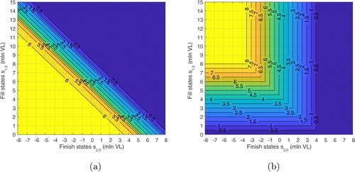
Table 3. Size of decision zones in response to yield uncertainty in fill-operations (in Θ).

		No	Lower	Higher	No	Higher
	Base Case	yield losses	yield losses	yield losses	variability	variability	All-or-Nothing
Fill zones
Zone I	0.35	0.28	0.30	0.91	0.33	0.46	0.78
Zone II	0.27	0.31	0.30	0.08	0.26	0.26	0.16
Zone III	0.38	0.41	0.41	0.01	0.41	0.28	0.06
Finish zones
Zone I	0.18	0.18	0.18	0.15	0.18	0.17	0.18
Zone II	0.25	0.24	0.24	0.29	0.27	0.25	0.25
Zone III	0.37	0.29	0.30	0.39	0.31	0.38	0.34
Zone IV	0.21	0.28	0.28	0.17	0.24	0.20	0.23

In Table 3, we observe that Zone I expands whereas Zone III shrinks as the yield uncertainty becomes higher in the system (i.e., as the average yield losses or process variability increase). This indicates that the fill-operation tends to buffer against uncertainty by increasing its production amounts. In contrast, finish zones exert a different response to yield uncertainty. For example, Zone I of finish-operations tend to shrink whereas Zone III expands as the average yield losses or yield variability increases. This implies that a finish-operation responds to the yield uncertainty of fill-operations by reducing its production amounts. The underlying intuition can be associated with several factors. For example, the cost of holding inventory in the finish station is more expensive than the cost of holding inventory in the fill station. In addition, note that the system already buffers against yield uncertainty of fill-operations by increasing the production amounts of fill-operations (i.e., Zone I of fill expands in Table 3 as the yield uncertainly increases).

6.3. Insights on freeze periods

To understand the impact of freeze period on costs and policies, the base case is solved with a freeze period of length $L\in \{2,3,4,5\}.$ Note that freeze periods with $L\ge 6$ are not considered in the numerical analysis, as they are not practical in our specific production setting. Currently, MSD AH uses a freeze period of L = 2. We consider planning activities for a year, i.e., $\omega \in \{1,\dots ,12\}.$ However, we also tested the sensitivity of optimal costs to longer planning activities and concluded that our insights are similar for a longer horizon of planning activities. At each planning activity, the biomanufacturer uses the most recent forecasts and generates a production plan for a planning horizon of 2 years, T = 24 (i.e., in alignment with Sections 6.1 and 6.2). To assess the impact of freeze periods at MSD AH, we used historical sales data and their corresponding forecast files (see the electronic companion for further details on the demand distribution). For example, the forecast file of January 2016 is used in the first planning activity ω = 1, whereas the forecast file of December 2016 is used in the last planning activity ω = 12. Our main objective is to quantify the financial impact of freezing the production decisions, and help practitioners to have a better understanding on the trade-off between planning stability and flexibility.

To quantify the impact of freeze periods, we use the percentage change in the (T-period) expected cost in a particular planning activity as a key performance metric. More specifically, for a given freeze period of length L, Table 4 shows the percentage increase in the (24-period) expected cost compared with the base case with no freeze periods at state ($s_1,s_2)$ in the first decision epoch of the planning activity ω = 6 (we consider this particular planning activity as an example that reflects a situation halfway in the series of monthly re-planning activities considered in the case study). First, we focus on the current practice, and assess the financial implications of using a freeze period of length L = 2. Table 4 shows that the percentage increase in the optimal cost (compared with the base case) can be up to 11.3% under a freeze period of length L = 2. Further analysis shows that this increase can be up to 20% considering all other states that are not covered in Table 4. In addition, we see that the percentage increases under L = 3 are at least 1.5 times higher compared with those under L = 2. Therefore, financial implications of the freeze period become more pronounced as the freeze period increases from 2 to 3 months.

Table 4. Percentage increase in the value function under different lengths L of freeze period.

s1	s2	L = 2	L = 3	L = 4	L = 5
0	−2	0.0	1.4	4.0	5.6
3	−2	1.0	10.6	12.2	19.6
6	−2	6.1	11.9	18.2	27.0
9	−2	7.3	12.9	21.0	30.0
0	0	0.7	6.8	9.7	15.3
3	0	4.6	8.2	12.6	19.5
6	0	7.8	18.5	29.5	42.0
9	0	1.8	18.6	26.7	36.3
0	2	5.9	11.9	18.5	29.9
3	2	11.3	18.7	29.0	39.7
6	2	4.4	34.8	31.2	45.2
9	2	2.2	19.0	27.3	34.8
0	4	8.2	16.0	24.6	36.4
3	4	9.8	17.2	28.1	40.2
6	4	2.0	16.8	30.6	43.9
9	4	1.8	14.4	22.1	25.8

Table 4 indicates that the percentage increase in costs gets higher in L for a fixed system state, however, no specific trends were observed regarding the behavior of the percentage increase as a function of the system state under a fixed L. On the other hand, at L = 2, we see that the highest percentage increase is often attained in a system state where the net inventory is around 5 to 7 mln VL– which often corresponds to states within Zone II. This behavior indicates that the demand information plays a more critical role in adjusting the production amounts in Zone II. When the production schedule is frozen in advance, decisions are made based on older demand information and can not be adjusted.

Results in Table 4 help operations managers understand the financial implications of the flexibility loss due to freeze periods. In practice, biomanufacturers often deal with a complex trade-off between planning flexibility and planning stability, and our analysis indicates that the current strategy of adopting a 2-month freeze period can lead up to a 20% increase in the expected cost of fill-and-finish operations considered in our specific case study. For practitioners, these results provide a rigorous and quantitative approach for assessing the impact of freezing production schedules, and enables an easier communication of planning strategies within the company.

7. Conclusions

Fill-and-finish operations include activities related to formulation, freeze-drying, filling, and sealing an active ingredient into its final form. State-of-the-art technologies can deliver consistent production yields in finish-operations. However, fill-operations remain a critical challenge in practice, as it relies on complex and unpredictable biological processes, such as freeze-drying. This leads to yield uncertainty in fill-operations. In addition, fill-and-finish operations are labor- and cost-intensive, and require specialized handling with strict limitations on batch sizes and capacity. As a response to these challenges, most biopharmaceutical companies tend to freeze their production decisions for a predefined period of time. This allows companies to improve their visibility and stability in manufacturing processes. However, using such freeze periods adds another level of challenge, as it reduces planning flexibility.

To address these problems, we develop a finite-horizon, discounted-cost Markov decision model that optimizes the production decisions at biopharmaceutical fill-and-finish operations. The model is then extended to optimize decision-making under freeze periods. We analyze the structural properties of the optimal costs and policies, and show that the state space can be partitioned into decision zones. More specifically, we show that optimal production decisions can be classified into three decision zones for fill-operations, and four decision zones for finish-operations. These decision zones provide guidelines on optimal policies, and are easy to implement in practice.

We present an industry case study, and focus on evaluating the impact of yield uncertainty on optimal costs and policies. In our specific case study, numerical experiments indicate that fully eliminating the yield uncertainty in fill-operations can provide 20% to 60% improvement (depending on the current inventory levels) in the expected cost of fill-and-finish operations. In a typical large scale biopharmaceutical setting, such room for improvement could often lead to a six figure reduction in costs. We note that companies can adopt new technologies to reduce yield uncertainty, but fully eliminating the yield uncertainty might not necessarily be feasible, due to of technological limitations. Nevertheless, our results provide a quantified business case to encourage further development in this field. We also conclude that the financial implications of controlling the yield variability can be as critical as controlling the mean yield losses themselves. In addition, numerical experiments reveal insights related to the cost of freezing the production decisions. In our specific case study, we observe that the current practice of adopting a 2-month freeze period could lead up to 20% increase in the expected costs of fill-and-finish operations.

This research has been conducted in close collaboration with MSD AH in the Netherlands. However, the true impact of this work extends beyond their operations, as it addresses common industry challenges and trade-offs. Insights obtained from this research have also been shared with a larger biotech community through working group sessions. Industry feedback indicates that most biomanufacturers rely on expert opinion and MRP calculations that have limited ability in incorporating the manufacturing challenges (e.g., yield and demand uncertainty) into decision-making. Therefore, we believe that the optimization framework presented in this article will help to improve decision-making in practice.

The application of Operations Research (OR) methodologies to the biomanufacturing industry is still in its infancy. However, biomanufacturers are realizing that they need to undergo a data-driven, OR-based transformation to fully realize the benefits of bioscience research. Future work could consider production and scheduling decisions for multiple products and/or multiple biomanufacturing activities (i.e., fermentation, chromatography, filtration, and fill-finish). In addition, the model can be extended to incorporate inventory spoilage into decision-making. We note that freeze-dried products (such as those considered in this article) have long shelf lives. However, several biopharmaceuticals, especially those in human health, might have limited shelf lives. Another potential research stream could combine demand learning mechanisms with production planning decisions for fill-and-finish operations.

Acknowledgments

We are grateful to the Department Editor, the Associate Editor, and two anonymous reviewers for their constructive comments on an earlier version of this article.

Additional information

Funding

This research has been funded by the Dutch Science Foundation, NWO-VENI Talent Scheme.

Notes on contributors

Tugce Martagan

Tugce Martagan is an assistant professor in the Department of Industrial Engineering and Innovation Sciences at Eindhoven University of Technology. She received her PhD in Industrial Engineering from the University of Wisconsin-Madison. Her research interests include healthcare operations, and design and optimization of biomanufacturing systems.

Alp Akcay

Alp Akcay is an assistant professor in the Department of Industrial Engineering and Innovation Sciences at Eindhoven University of Technology. He received his PhD in operations management from the Tepper School of Business at Carnegie Mellon University. His research interests include decision making under uncertainty in applications such as planning and control of manufacturing systems and predictive maintenance for capital goods.

Maarten Koek

Maarten Koek is a planning lead at MSD Pharm Ops in the Netherlands. He received his BSc in industrial engineering and MSc in operations management and logistics from Eindhoven University of Technology. His research interests include stochastic modeling and specifically Markov decision processes. His projects focus on applying theoretically proven concepts to problems faced by professionals within the bio-pharmaceutical industry.

Ivo Adan

Ivo Adan is a professor at the Department of Industrial Engineering of the Eindhoven University of Technology. His current research interests are in modeling, design and control of manufacturing systems, warehousing systems and transportation systems, and more specifically, in the analysis of multi-dimensional Markov processes and queueing models.

Appendix:

Proofs

Proof of Lemma 1.

Notice that the $L^{♮}$-convexity of the function $g(\mathbf{v},\xi )$ is equivalent to the $L^{♮}$-convexity of the function $\psi (\mathbf{v},\xi r)$ in v and ξ. It follows from the definition of $L^{♮}$-convexity that the latter is the case if (10) $$\psi \left(\left[\begin{array}{c}{v}_1-\epsilon \\ \dots \\ v_n-\epsilon \\ \xi r-\epsilon \end{array}\right]\right)=f\left(\left[\begin{array}{c}{v}_1-\epsilon -(\xi r-\epsilon )\\ \dots \\ v_n-\epsilon -(\xi r-\epsilon )\end{array}\right]\right)=f\left(\left[\begin{array}{c}{v}_1-\xi r\\ \dots \\ v_n-\xi r\end{array}\right]\right)$$(10) is submodular in $\mathbf{v}=(v_1,\dots ,v_n)$ and ξ. Let $h(v_1,\dots ,v_n,\xi )$ denote the function $f(v_1-\xi ,\dots ,v_n-\xi ).$ It is known that submodularity is invariant by separable strictly increasing reparameterizations, that is, if $\phi (·)$ is a strictly increasing bijection, the function $h(v_1,\dots ,v_n,\xi )$ is submodular, if and only if, the function $h(v_1,\dots ,v_n,\phi (\xi ))$ is submodular (Bach, 2019). It follows from Lemma 1 of Zipkin (2008) that the function $h(v_1,\dots ,v_n,\xi )$ is submodular, and hence the result follows. □

Proof of Theorem 1.

(i) Notice that the terminal value function $J_T(w_1,w_2)$ is the sum of linear functions and hence is $L^{♮}$-convex. We assume, as the induction hypothesis, that the function $J_{t+1}$ is $L^{♮}$-convex. From Lemma 1, we know that $J_{t+1}({\overline{w}}_1-\xi r,w_2-\xi r)$ is $L^{♮}$-convex in ${\overline{w}}_1,$ w₂, and ξ for $r\ge 0.$ Therefore, the function $J_{t+1}({\overline{w}}_1-\xi r-y,w_2-\xi r-y)$ is submodular in ${\overline{w}}_1,$ w₂, ξ and y. Since submodularity is invariant by separable strictly increasing reparameterizations, it is known that the function $J_{t+1}({\overline{w}}_1-\xi r-y,w_2-\xi r-d-y)$ is also submodular in ${\overline{w}}_1,$ w₂, ξ and y. Thus, it follows from Proposition 3 of Chen (2017) that the function $J_{t+1}({\overline{w}}_1-\xi r,w_2-\xi r-d)$ continues to be $L^{♮}$-convex in ${\overline{w}}_1,$ w₂, and ξ for a constant d. Because the expectation operator preserves $L^{♮}$-convexity, it follows that the objective function in the optimization problem (11) $$\begin{array}{c}{\tilde{J}}_{t+1}(w_1,w_2,\xi )=\underset{{\overline{w}}_1}{\text{min}}\mathbb{E}\left[J_{t+1}({\overline{w}}_1-\xi R,w_2-\xi R-D_t)\right]\\ \mathrm{s}.\mathrm{t}.-m_2{b}_2\le {\overline{w}}_1-w_1\le 0\\ 0\le {\overline{w}}_1\end{array}$$(11) is also $L^{♮}$-convex in $w_1,{\overline{w}}_1,w_2$ and ξ. Consequently, it follows from Lemma 2(b) of Huh and Janakiraman (2010) that the function ${\tilde{J}}_{t+1}(w_1,w_2,\xi )$ is $L^{♮}$-convex in w₁, w₂ and ξ. Furthermore, consider the optimization problem (12) $$\begin{array}{c}{f}_{t+1}(w_1,w_2)=\underset{\xi }{\text{min}}{\tilde{J}}_{t+1}(w_1,w_2,\xi )\\ \mathrm{s}.\mathrm{t}.-m_1{b}_1\le \xi \le 0\end{array}$$(12)

It again follows from Lemma 2(b) of Huh and Janakiraman (2010) that the function $f_{t+1}(w_1,w_2)$ is $L^{♮}$-convex in w₁ and w₂. Consequently, the value function $J_t(w_1,w_2)$ in (6) is the sum of $L^{♮}$-convex functions, and therefore, it is $L^{♮}$-convex, completing the induction.

1. Let ${\xi }_t^{*}(w_1,w_2)$ denote the largest minimizer of the objective function in (12(12) $$\begin{array}{c}{f}_{t+1}(w_1,w_2)=\underset{\xi }{\text{min}}{\tilde{J}}_{t+1}(w_1,w_2,\xi )\\ \mathrm{s}.\mathrm{t}.-m_1{b}_1\le \xi \le 0\end{array}$$(12) ) for some t. Since the objective function in (12(12) $$\begin{array}{c}{f}_{t+1}(w_1,w_2)=\underset{\xi }{\text{min}}{\tilde{J}}_{t+1}(w_1,w_2,\xi )\\ \mathrm{s}.\mathrm{t}.-m_1{b}_1\le \xi \le 0\end{array}$$(12) ) is submodular (due to its $L^{♮}$-convexity) and the feasible region forms a lattice, Topkis’ monotonicity theorem (Theorem 2.8.2, Topkis (1998)) implies that ${\xi }_t^{*}(w_1,w_2)$ is nondecreasing in w₁ for a fixed w₂, and it is nondecreasing in w₂ for a fixed w₁. Let $u_{1,t}^{*}(s_1,s_2)=-{\xi }_t^{*}(w_1,w_2),$ where the relations between $w_1,w_2,s_1$ and s₂ are already defined by the state transformation. Since ${\xi }_t^{*}$ is nondecreasing in w₁, and w₁ is equal to s₁, $u_{1,t}^{*}(s_1,s_2)$ is nonincreasing in s₁. Furthermore, since ${\xi }_t^{*}$ is nondecreasing in w₂, and w₂ is nondecreasing in s₂, $u_{1,t}^{*}(s_1,s_2)$ is nonincreasing in s₂. □

Proof of Theorem 2.

We prove the result first for all-or-nothing type of yield uncertainty and then for deterministic yield.

All-or-nothing yield. (i) The terminal value function $J_T(w_1,w_2)$ is the sum of linear functions and hence is $L^{♮}$-convex. We assume, as induction hypothesis, that the function $J_{t+1}$ is $L^{♮}$-convex. From Lemma 1 (with r = 1), we know that $J_{t+1}({\overline{w}}_1-\xi ,w_2-\xi )$ is $L^{♮}$-convex in ${\overline{w}}_1,$ w₂, and ξ and that $J_{t+1}(w_1-\xi ,w_2-\xi )$ is $L^{♮}$-convex in w₁, w₂, and ξ. As shown in the proof of Theorem 1, for a constant d, the function $J_{t+1}({\overline{w}}_1-\xi ,w_2-\xi -d)$ is $L^{♮}$-convex in ${\overline{w}}_1,$ w₂, and ξ, and the function $J_{t+1}(w_1-\xi ,w_2-\xi -d)$ is $L^{♮}$-convex in w₁, w₂, and ξ. Thus, the function $$q({\overline{w}}_1,w_1,w_2,\xi ;d)\triangleq \mathbb{P}(R=1)J_{t+1}({\overline{w}}_1-\xi ,w_2-\xi -d)+\mathbb{P}(R=0)J_{t+1}(w_1-\xi ,w_2-\xi -d),$$ is $L^{♮}$-convex in ${\overline{w}}_1,$ w₁, w₂, and ξ for a constant d. Because the expectation operator preserves $L^{♮}$-convexity, it follows that the objective function in the optimization problem (13) $$\begin{array}{c}{\tilde{J}}_{t+1}(w_1,w_2,\xi )=\underset{{\overline{w}}_1}{\text{min}}\mathbb{E}\left[q({\overline{w}}_1,w_1,w_2,\xi ;D_t)\right]\\ \mathrm{s}.\mathrm{t}.w_1-{\overline{w}}_1\le m_1{b}_1,\end{array}$$(13) is also $L^{♮}$-convex in $w_1,{\overline{w}}_1,w_2$ and ξ. Consequently, it follows from Lemma 2(b) of Huh and Janakiraman (2010) that the function ${\tilde{J}}_{t+1}(w_1,w_2,\xi )$ is $L^{♮}$-convex in w₁, w₂ and ξ. Furthermore, consider the optimization problem (14) $$\begin{array}{c}{f}_{t+1}(w_1,w_2)=\underset{\xi }{\text{min}}{\tilde{J}}_{t+1}(w_1,w_2,\xi ),\\ \mathrm{s}.\mathrm{t}.-m_2{b}_2\le \xi \le 0,\\ w_1-\xi \le 0.\end{array}$$(14)

It again follows from Lemma 2(b) of Huh and Janakiraman (2010) that the function $f_{t+1}(w_1,w_2)$ is $L^{♮}$-convex in w₁ and w₂. Consequently, the value function $J_t(w_1,w_2)$ in (8(8) $$J_t(w_1,w_2)=c(-w_1,w_2)+\gamma f_{t+1}(w_1,w_2),$$(8) ) is the sum of $L^{♮}$-convex functions, and therefore, it is $L^{♮}$-convex, completing the induction.

(ii) Let ${\xi }_t^{*}(w_1,w_2)$ denote the largest minimizer of the objective function in (14(14) $$\begin{array}{c}{f}_{t+1}(w_1,w_2)=\underset{\xi }{\text{min}}{\tilde{J}}_{t+1}(w_1,w_2,\xi ),\\ \mathrm{s}.\mathrm{t}.-m_2{b}_2\le \xi \le 0,\\ w_1-\xi \le 0.\end{array}$$(14) ) for some t. Since the objective function in (14) is submodular (due to its $L^{♮}$-convexity) and the feasible region forms a lattice, Topkis’ monotonicity theorem (Theorem 2.8.2, Topkis (1998)) implies that ${\xi }_t^{*}(w_1,w_2)$ is nondecreasing in w₁ for a fixed w₂, and it is nondecreasing in w₂ for a fixed w₁. Let $u_{2,t}^{*}(s_1,s_2)=-{\xi }_t^{*}(w_1,w_2),$ where the relations between $w_1,w_2,s_1$ and s₂ are already defined by the state transformation. Since ${\xi }_t^{*}$ is nondecreasing in w₁, and w₁ is equal to $-s_1,u_{2,t}^{*}(s_1,s_2)$ is nondecreasing in s₁. Furthermore, since ${\xi }_t^{*}$ is nondecreasing in w₂, and w₂ is equal to s₂, $u_{2,t}^{*}(s_1,s_2)$ is nonincreasing in s₂. Thus, the result follows.

Deterministic yield. The result immediately follows from the analysis of the full-yield case (i.e., $\mathbb{P}(R=1)=1$ under all-or-nothing yield uncertainty). In the deterministic case, the yield is known upfront, suppose its value is r. The optimal finish policy in the full-yield case, which is solved under the finish capacity $m_2{b}_{2}r,$ can be transformed (by multiplying with $1/r$) to obtain the optimal finish policy of the case with yield r. Since this transformation keeps the monotonicity of the finish policy, and the monotonicity of the finish for the full-yield case is already shown above, the result follows. □

References

- Bach, F. (2019) Submodular functions: from discrete to continuous domains. Mathematical Programming, 175(1-2), 419–459.
- Bollopragada, S. and Morton, T.E. (1999) Myopic heuristics for the random yield problem. Operations Research, 47(5), 713–722.
- Chen, X. (2017) L♮-convexity and its applications in operations. Frontiers of Engineering Management, 2.
- Clark, A.J. and Herbert Scarf, H. (1960) Optimal policies for a multi-echelon inventory problem. Management Science, 6(4), 475–490.
- Ehrhardt, R. and Taube, L. (1987) An inventory model with random replenishment quantities. International Journal of Production Research, 25(12), 1795–1803.
- Gong, X. and Chao, X. (2013) Optimal control policy for capacitated inventory systems with remanufacturing. Operations Research, 61(3), 603–611.
- Gutka, H. and Prasad, K. (2015) Current Trends and Advances in Bulk Crystallization and Freeze-Drying of Biopharmaceuticals. Springer, New York, NY, pp. 299–317.
- Han, G., Dong, M. and Shao, X. (2012) Yield management with downward substitution and uncertainty demand in semiconductor manufacturing. International Journal of Production Research, 50(3), 743–756.
- Henig, M. and Gerchak, Y. (1990) The structure of periodic review policies in the presence of random yield. Operations Research, 38(4), 634–643.
- Huh, W.T. and Janakiraman, G. (2010) On the optimal policy structure in serial inventory systems with lost sales. Operations Research, 58(2), 486–491.
- Hwang, J. and Singh, M.R. (1998) Optimal production policies for multi-stage systems with setup costs and uncertain capacities. Management Science, 44(9), 1279–1294.
- Inderfurth, K. (2004) Analytical solution for a single-period production-inventory problem with uniformly distributed yield and demand. Central European Journal of Operations Research, 12(2), 117–127.
- Janakiraman, G. and Muckstadt, J.A. (2009) A decomposition approach for a class of capacitated serial systems. Operations Research, 57(6), 1384–1393.
- Jiang, G., Thummala, A. and Wadhwa, M.V.S. (2011) Applications of statistical regression and modeling in fill–finish process development of structurally related proteins. Journal of Pharmaceutical Science, 100(2), 464–481.
- Käki, A,. Liesiö, J., Salo, A. and Talluri, S. (2015) Newsvendor decisions under supply uncertainty. International Journal of Production Research, 53(3), 1544–1560.
- Karlin, S. (1958) One stage inventory models with uncertainty. In S. Karlin K. J. Arrow and H. Scarf (ed.), Studies in the Mathematical Theory and Inventory and Production, Stanford University Press, Stanford, CA, pp. 109–134.
- Khairuddin, N.L., Norliza Abd Rahman, N.A. and Kamarudin, N.S. (2016) Design of fill and finish facility for active pharmaceutical ingredients (api). Journal of Engineering Science and Technology, 11(8), 1135–1154.
- Kogan, K. and Lou, S. (2003) Multi-stage newsboy problem: A dynamic model. European Journal of Operational Research, 149(2), 448–458.
- Langer, E. (2016) Fill/finish outsourcing. Pharmaceutical Technology, 40(10), 74–77.
- Li, Q. and Yu, P. (2014) Multimodularity and its applications in three stochastic dynamic inventory problems. Manufacturing & Service Operations Management, 16(3), 455–463.
- Martagan, T., Krishnamurthy, A. and Maravelias, C.T. (2016) Optimal condition-based harvesting policies for biomanufacturing operations with failure risks. IIE Transactions, 48(5), 440–461.
- Mazzola, J.B., McCroy, W.F. and Wagner, H.M. (1987) Algorithms and heuristics for variable-yield lot sizing. Naval Research Logistics, 34, 67–86.
- McLeod, L.D., Montgomery, S.A. and Scott, C. (2011) Fill and finish for biologics. http://www.bioprocessintl.com/manufacturing/fill-finish/fill-and-finish-for-biologics-316516/?pageNum=2. Accessed July 8, 2018.
- Miller, M. (2009) Quality risk management and the economics of implementing rapid microbiological methods. European Pharmaceutical Review, 2, 66–73.
- Nederlandse Biotechnologische Vereniging. (2018) Computers and bioprocess development. https://nbv.kncv.nl/en/activities/nbv-detail-page/411/computers-bioprocess-development/about. Accessed March, 28 2018.
- Noori, H. and Keller, G. (1986) One-period order quantity strategy with uncertain match between the amount received and quantity requisitioned. INFOR: Information Systems and Operational Research, 24(1), 1–11.
- Papachristos, S. and Katsaros, A. (2008) A periodic-review inventory model in a fluctuating environment. IIE Transactions, 40(3), 356–366.
- Parker, R. and Kapuscinski, R. (2004) Optimal policies for a capacitated two-echelon inventory system. Operations Research, 52(5), 739–755.
- Patro, S.Y., Freund, E. and Chang, B.S. (2002) Protein formulation and fill-finish operations. Biotechnology Annual Review, 8, 55–84.
- Petrides, D., Siletti, C., Jiménez, J., Psathas, P. and Mannion, Y. (2011) Optimizing the design of operation of fill-finish facilities using process simulation and scheduling tools. Pharmaceutical Engineering, 31(2), 1–10.
- Rathore, A.S. and Mhatre, R. (2011) Quality by Design for Biopharmaceuticals: Principles and Case Studies, vol. 1. John Wiley & Sons, Hoboken, NJ.
- Rekik, Y., Sahin, E. and Dallery, Y. (2007) A comprehensive analysis of the newsvendor model with unreliable supply. OR Spectrum, 29(2), 207–233.
- Rios, M. (2012) A decade of fill–finish and packaging solutions. BioProcess International, 10(6), 54–56.
- Robinson, J., Miller, S., Baxter, L.T., Hunt, S., Todd, B. and Pekny, J.F. (2017) Using simulation to address capacity limitations. Biopharm International, 30(9), 18–22.
- Schmitt, A.J. and Snyder, L.V. (2012) Infinite-horizon models for inventory control under yield uncertainty and disruptions. Computers and Operation Research, 39(4), 850–862.
- Scott, C. and Rios, M. (2015) Bioprocess theater: Formulation, fill and finish. http://www.bioprocessintl.com/2015/may-2015-supplement/bioprocess-theater-formulation-fill-and-finish/ Accessed August 24, 2018.
- Simchi-Levi, D., Xin Chen, X. and Bramel, J. (2014) Convexity and supermodularity, in The Logic of Logistics. Springer, New York, NY, pp.15–44.
- Tang, C.S. (1990) The impact of uncertainty on a production line. Management Science, 36(12), 1518–1531.
- Tomlin, B. (2009) Impact of supply learning when suppliers are unreliable. Manufacturing & Service Operations Management, 11(2), 192–209.
- Topkis, D.M. (1998) Supermodularity and Complementarity, Princeton University Press, Princeton, NJ.
- Yano, C.A. and Lee, H.A. (1995) Lot sizing with random yield: A review. Operations Research, 43(2), 311–334.
- Zanjani, M.K., Ait-kadi, D. and Nourelfath, M. (2010) Robust production planning in a manufacturing environment with random yield: A case in sawmill production planning. European Journal of Operational Research, 201(3), 882–891.
- Zanjani, M.K., Nourelfath, M. and Ait-kadi, D. (2010) A multi-stage stochastic programming approach for production planning with uncertainty in the quality of raw materials and demand. International Journal of Production Research, 48(16), 4701–4723.
- Zipkin, P. (2008) On the structure of lost-sales inventory models. Operations Research, 56(4), 937–944.