Reducing risks in spare parts service contracts with a long downtime constraint

Abstract

This article investigates spare parts service contracts for capital goods. We consider a single-item, single-location inventory system that serves one customer with multiple machines. During the contract execution phase, the true demand rate is observed. It can differ from the estimated demand rate because of two factors: increased demand variation in finite horizon settings and a shift in the mean utilization of the machines by the user during the contract. When the true demand rate is higher than the estimated demand rate, the Original Equipment Manufacturer (OEM) is faced with higher-than-expected costs for the execution of the contract, and the asset user is generally faced with a higher number of extreme long downtime events. Therefore, we introduce the flexible-time contract, which ends after a predetermined number of demands. Using a Markov decision process, we prove that a state-dependent base stock policy is optimal under a flexible-time contract. Using simulation, we compare the flexible-time contract with the standard fixed-time contract. Our results show that the flexible-time contract reduces the costs for the OEM by up to 35% and prevents not meeting the agreed-on service level. We obtain similar results in a multi-item setting.

Keywords:

• Spare parts service contracts
• spare parts inventory
• optimal policy
• multimodularity
• costs variation

1. Introduction

Users of capital goods rely on diverse equipment from Original Equipment Manufacturers (OEMs) to deliver their products or services. For example, industrial companies need manufacturing equipment, and hospitals need diagnostic, life support and laboratory equipment. With capital goods becoming more and more complex, their maintenance and supporting spare parts supply chains are increasingly being outsourced (Pascual et al., 2016). Drawing on our observations in the practice of ASML, a supplier of photo-lithography equipment for the semiconductor industry, we identify four challenges faced by OEMs and their customers.

First, maintenance and enabling service supply chains should work to prevent long interruptions. Most users require stable operations, and long infrequent interruptions are more harmful than short frequent ones (Hopp and Spearman, 2011). The commonly used spare parts service measures are Aggregate Fill Rate (AFR), aggregate mean waiting time, and variants of them. In the semiconductor industry, for example, DownTime Waiting for Parts (DTWP) has been the standard for more than a decade and is a variant of the aggregate mean waiting time. Under AFR, there is no commitment from the OEM on how long the customer needs to wait in the case where the component is not delivered directly from stock. Under DTWP, the commitment is on the mean, so the OEM can compensate a slow delivery with multiple fast deliveries. In this article, we consider a spare parts service contract under an extreme Long Downtime (XLD) service constraint. This constraint, which was introduced by Lamghari-Idrissi, Basten and van Houtum (2020), limits the number of times during the contract period that the system downtime is longer than an agreed-on threshold. The asset user and the OEM set a downtime duration threshold and the maximum number of times the threshold can be exceeded during the contract period. Should the threshold be exceeded more than the agreed-on number of times, the service provider pays a penalty for every new downtime exceeding the threshold. Lamghari-Idrissi, Basten and van Houtum (2020) derive the structure of the optimal policy in a finite time horizon setting. To determine the benefits of the XLD service constraint, Lamghari-Idrissi, Basten, Dellaert and van Houtum (2020) compare the XLD service measure with AFR and DTWP. As an XLD constraint is the only service constraint that sets a limit on how often the time to repair can exceed an agreed-on threshold, it decreases the coefficient of variation of the time to repair by up to 35%, resulting in a lower cycle time and work-in-progress inventory in the factory of the asset user (Lamghari-Idrissi, Basten, Dellaert and van Houtum 2020).

Second, demand rates are typically underestimated in the contracting phase. Before a service contract is signed, the OEM receives from the asset user an estimated utilization level of the machines over the agreed-on contract duration. Estimating this level is difficult, because the semiconductor market is highly cyclical. The start of a cycle, its duration, and its magnitude can be very challenging to predict. In addition, chip manufacturers often go through bidding processes to secure new sales volumes, adding to the difficulty of estimating a utilization level (Geng and Jiang, 2009; Mönch et al., 2018), and they tend to be conservative in the contracting phase when estimating the expected utilization level of the systems (Hyvönen and Järvinen, 2006; Koch et al., 2009). As it is based on the estimated utilization level from the asset user, the expected spare parts demand rate the OEM uses in the contracting phase is often lower than the true spare parts demand rate during the execution phase of the contract. In a literature review of quantitative models for supply chain risks, Fahimnia et al. (2015) show that the difficulty in estimating the demand rate is a leading source of risk in contracting; yet it has received limited attention in the literature (Van Der Auweraer et al., 2019; Song et al., 2020). When the demand rate is underestimated, the OEM potentially keeps a relatively low spare parts stock at the site of the customer and may be faced with high penalties because the agreed-on service level is not met. For the asset user, exceeding the number of XLDs can have a devastating impact on its operations, which is typically more costly than the penalties paid out by the OEM. In a modern front-end wafer fab, for example, it takes approximately 3 weeks for the production to recover from a 24-hour unscheduled downtime. Hishamuddin et al. (2012) show that the recovery costs increase exponentially as a function of the disruption duration for a single-stage production-inventory system. Front-end wafer fabs are multi-stage production-inventory systems with re-entrant flows, reinforcing these results. As penalty costs represent only a fraction of the real customer impact, underestimating the utilization levels of the systems by the asset user and, thus, the spare parts demand rate by the OEM is a joint problem for the parties involved. This is in line with the findings of Gebauer et al. (2017) for cost-plus contracts and Visnjic et al. (2017) for performance-based contracts.

Third, service contracts are always defined over a finite horizon. Spare parts inventory control in a finite horizon setting has received less attention in the literature than inventory control in the infinite horizon setting (Hu et al., 2018). In a finite horizon setting, the achieved performance is a random variable. This is an additional challenge that arises even when the demand rate estimate is accurate and this can heavily influence the costs of a contract (Cohen and Agrawal, 1999; Kim and Park, 2008). Tan et al. (2017) prove that in order to meet the same target fill rate level, the inventory level increases as the performance review horizon decreases.

The fourth challenge is building proper incentive structures in service contracts. In the semiconductor industry, this challenge is exacerbated by the high reliability of the systems (Kim et al., 2010). With highly reliable high-tech systems, the probability of failure of a component is extremely low, resulting in high demand uncertainty. Risk pooling is an established practice to help temper the effects of demand uncertainty (Mak and Shen, 2012). Gerchak and He (2003) show analytically that the benefits of risk pooling increase as the demand uncertainty increases.

To mitigate the four challenges described, we investigate an alternative form of contracts using the XLD service measure. Instead of defining the contract over a pre-agreed-on period (as for fixed-time contracts), we propose defining a spare parts service contract over a pre-agreed-on spare parts demand, resulting in a variable time duration. The primary objective of our proposed flexible-time contract is to reduce the mean costs associated with delivering a spare parts service contract. A secondary objective is to reduce the mean number of XLDs. By defining the contract over a pre-defined number of spare parts demand, determining the expected costs is more directly linked to the service being provided. This should help reduce the risks for the OEMs in terms of costs and for the asset user in terms of performance.

We consider a periodic review inventory model in a single-item, single-location stockpoint setting serving multiple systems. The demand per period for all systems together follows a binomial distribution. Should the stockpoint be out of stock when the demand arrives, it can be satisfied from an emergency warehouse, against additional costs. The emergency warehouse is assumed to have ample stock.

To the best of our knowledge, flexible-time contracts have not been investigated in the literature. We aim to answer the following questions:

1. What is the structure of the optimal inventory policy under a flexible-time contract?

2. How does the flexible-time contract perform compared with the traditional fixed-time contract under an accurate demand rate estimate?

3. How do flexible-time and fixed-time contracts perform when the demand rate is underestimated?

4. What is the impact of updating the demand rate forecast on the performance of the two contracts? And

5. How do the results extend to a multi-item setting?

Our contribution is five-fold. First, we derive the optimal policy for a flexible-time contract with an XLD service constraint. We prove the optimality of a state-dependent base stock policy, in which the state is given by the remaining allowed number of long downtimes and the remaining length of the contract period (expressed in remaining total spare parts demand). Second, using simulation, we compare the costs of fixed-time and flexible-time contracts under an accurate demand rate estimate. We show that the costs under a flexible-time contract are lower than the costs under a fixed-time contract, though not considerably. Third, we compare the costs of the contracts for the case when the true demand rate is higher than the estimated demand rate (i.e., when the asset user has underestimated the utilization level). Our results show that when the true demand rate is 25% higher than the expected demand rate, the mean costs and mean number of XLDs under a flexible-time contract are up to 35% and 20% lower, respectively, than those under a fixed-time contract. Fourth, during the contract execution phase and depending on the observed demand rate, the OEM can adjust the inventory level. Therefore, in a separate numerical experiment, we extend our simulation to a setting in which the demand rate is updated. We observe that the mean costs for both contract types decrease, but the costs differences between the two contract types remain similar (i.e., also in this setting, flexible-time contracts are much less expensive). Fifth, we examine the effect of moving to a multi-item setting. We calculate the optimal stocking policy for a multi-item XLD model for both the fixed-time and flexible-time contracts. Our results show that the costs differences between the two contract types remain similar.

This article proceeds as follows: In Section 2, we introduce our model and formulate it as a Markov Decision Process (MDP). We derive the optimal policy structure in Section 3. In Section 4, we numerically show the improved performance of the flexible-time contract under an accurate demand rate estimate. In Section 5, we compare the flexible-time and fixed-time contracts when the demand rate has been underestimated. Section 6 analyses the impact of updating the demand rate forecast during the contract. In Section 7, we extend our results to a multi-item setting. We conclude in Section 8. Supplementary materials containing the proofs and the multi-item formulation are available for this article.

2. Model

2.1. Description and assumptions

We consider a single-item stockpoint that fulfills demand from an installed base of N ($\in {\mathbb{Z}}^{+}$) systems in the field. All systems are of the same type and all belong to the same customer. A contract is closed with this customer and applies to the total demand of the N systems. The contract covers a critical module or component of the system, meaning that upon failure, the system comes to a halt until the defective component is swapped for a functioning one. We use the XLD constraint, introduced by Lamghari-Idrissi, Basten and van Houtum (2020), to set the service level. The XLD service constraint limits the number of outliers in the time to repair. We assume that the diagnostic, swap, and recovery times are deterministic, in line with the spare parts focus of this article. Time is divided into periods of equal length and replenishment decisions can be taken at the beginning of each period. Between two decision epochs, the total demand can be higher than one. We define the total number of orders received over the contract duration as the “number of demands”. The contract allows for a maximum number of demands $K^{\text{obj}}\in {\mathbb{Z}}^{+}$ to be fulfilled later than a predefined time threshold (e.g., 12 hours) over an agreed-on number of spare parts demands called contract coverage. The contract coverage is denoted by F (e.g., 50 demands). Let $\mathrm{F}=\{0,1,\dots ,F\}.$ Should the limit for the XLDs be exceeded, penalty costs, $c^{\mathrm{p}},$ are incurred for every XLD above the target.

The stockpoint is replenished by a regional or central stockpoint of the OEM. The replenishment lead time is significantly shorter than the time between two decision epochs. As a consequence, we consider the replenishment lead time to be equal to zero. The stockpoint is close enough to the customer to neglect the shipment time from the stockpoint to the systems of the customer. When a demand is fulfilled by the local stockpoint, the failed system is operational again within the agreed-on time threshold. When the demand cannot be fulfilled by the local stockpoint, it is a lost sale for the local stockpoint and gets fulfilled by an emergency shipment from another location against additional costs $c^{\mathrm{e}}.$ We assume that every emergency shipment is a late delivery and therefore results in an XLD. The emergency shipment costs are typically low in comparison with the penalty costs. This is in line with practice in which XLDs have a devastating impact on the asset users’ operations.

We keep track of the number of demands remaining until the end of the contract, $U\in \mathrm{F}.$ We assume that each period is much shorter than the total contract duration. In a real-life setting, a period may be a week. We also assume low failure rates, which is a common assumption for capital goods. Therefore, we assume that each system can fail only once per period with probability p and will be repaired within the same period. This means that, during a period, the demand cannot exceed the number of systems in the installed base.

At the beginning of each period, the level to which the inventory is increased, S, is reassessed on the basis of three parameters: the remaining amount of demand until the contract stops, U; the current contract performance, K (i.e., the number of late deliveries still allowed for the remaining contract duration); and the current on-hand stock, I. As the replenishment lead time is equal to zero, it is never optimal for the stock level at the start of the period, S, to be higher than the minimum of N and U. Further, S cannot be lower than I. Let $c^{\mathrm{h}}$ denote the holding costs comprising storage costs, insurance costs, and the costs of tied-up capital. The holding costs are paid at the end of each period on the remaining on-hand inventory.

Let X be the number of system failures in a period (i.e., the observed demand for the stockpoint). X is a binomially distributed random variable with parameters N and p: $$\mathbb{P}\left\{X=x\right\}=\frac{N!}{(N-x)!x!}{p}^x{(1-p)}^{N-x}.$$

During each period, the demand covered by the contract will be equal to the actual observed demand until the period in which the number of remaining failures covered by the contract becomes smaller than the installed base. From that period onward, the demand covered by the contract will be equal to the actual observed demand or the remaining contract coverage. We define X_U as the demand that is covered by the scope of the contract: $$X_U=\{\begin{array}{cc}\min \{X,U\},\hfill & U=1,2,\dots ,N-1;\hfill \\ X,\hfill & U\ge N.\hfill \end{array}$$

When U < N, we have $\mathbb{P}\left\{X_U=x\right\}=0$ for $x=U+1,\dots ,N,$ and $\mathbb{P}\left\{X_U=U\right\}={\sum }_{x=U}^N\mathbb{P}\left\{X=x\right\}.$

The sequence of events in each period is as follows:

• The state, consisting of U, K, and I, is observed.

• Spare parts are ordered and received.

• Demand during the period is observed and fulfilled:

  • - The total demand is fulfilled from stock if $X_U\le I;$

  • - In case $X_U>I,$ I demands are fulfilled from stock, while the other demands are fulfilled by an emergency shipment (lost sale to the stockpoint);

• All costs are incurred.

Our objective is to derive the optimal inventory control policy.

2.2. MDP formulation

Our optimization problem can be formulated as a finite-state, discrete-time MDP. Let $\mathrm{K}=\{0,1,\dots ,K^{\text{obj}}\}$ be the set of allowed late deliveries and let $\mathrm{S}=\{0,1,\dots ,N\}$ be the set of possible stock levels. We define the lattice $\mathrm{L}=\mathrm{K}\times \mathrm{S}.$ Let $V(U,K,I)$ be the optimal remaining costs until the end of the contract when the system is in state (U, K, I) at the start of a period. After the OEM orders up to S, the direct expected costs in the period are: $$C(U,K,S)=\sum _{x=0}^N\mathbb{P}\left\{X_U=x\right\}c(K,S,x),U\in \mathrm{F}\backslash \left\{0\right\},(K,S)\in \mathcal{L},$$ where $c(K,S,x)=c^{\mathrm{h}}{(S-x)}^{+}+c^{\mathrm{e}}{(x-S)}^{+}+c^{\mathrm{p}}{(x-S-K)}^{+}.$

We define, for $U\in \mathrm{F}\backslash \left\{0\right\}$ and $(K,S)\in \mathrm{L}:$ (1) $$\tilde{V}(U,K,S)=C(U,K,S)+\sum _{x=0}^N\mathbb{P}\left\{X_U=x\right\}V(U-x,{(K-{(x-S)}^{+})}^{+},{(S-x)}^{+}).$$(1)

The Bellman equation for our optimization problem is given by: (2) $$\begin{array}{c}V(U,K,I)=\underset{S\in \{I,\dots ,N\}}{\min }\tilde{V}(U,K,S),U\in \mathrm{F}\backslash \left\{0\right\},(K,I)\in \mathrm{L},\\ V(0,K,I)=0,(K,I)\in \mathrm{L}.\end{array}$$(2)

The total expected costs over the contract are given by $V(F,K^{\text{obj}},0).$

2.3. Reformulation of the Bellman equation

In this section, we make use of the structure of our problem to reformulate $\tilde{V}(U,K,S).$ This reformulation allows us to reduce the computational complexity of the optimal policy. Another limitation of the current Bellman equation is that it has four transitions to the same state, in the case of zero demand between two decisions epochs. As a consequence, proceeding by induction to prove the structure of the optimal policy is not possible. The reformulation of this section allows us to prove the properties of Section 3.

As $U\in \mathrm{F},K\in \mathrm{K},$ and $I\in \mathrm{S},$ we have a finite state space. In addition, the action space is finite because $S\in \{I,\dots ,N\}\subseteq \mathrm{S}.$ For all states for which U = 0, $V(U,K,I)=0.$ For $U\in \mathrm{F}\backslash \left\{0\right\},$ let $S^{*}(U,K,I)$ denote the smallest optimal action in state (U, K, I).

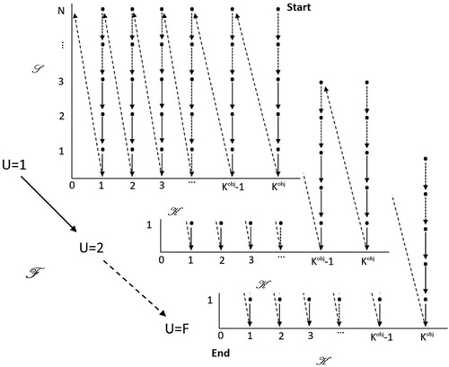
As Figure 1 illustrates, for $U\in \mathrm{F}\backslash \left\{0\right\},$ using backward induction on U, we can calculate all $\tilde{V}(U,K,S)$ directly with Equation (1)(1) $$\tilde{V}(U,K,S)=C(U,K,S)+\sum _{x=0}^N\mathbb{P}\left\{X_U=x\right\}V(U-x,{(K-{(x-S)}^{+})}^{+},{(S-x)}^{+}).$$(1) , except that we lack the expected costs associated with a transition to the same state, that is, when $I=S^{*}(U,K,I)$ and x = 0. We solve this problem as follows: We first calculate $\tilde{V}(1,K^{\text{obj}},N).$ In state $(1,K^{\text{obj}},N),$ the only possible action is to keep the same stock level (i.e., S = I = N). As a result, $V(1,K^{\text{obj}},N)=\tilde{V}(1,K^{\text{obj}},N).$ We have: $$\begin{array}{c}\tilde{V}(1,K^{\text{obj}},N)=\sum _{x=0}^N\mathbb{P}\{X_U=x\}(c^{\mathrm{h}}{(N-x)}^{+}{c}^{\mathrm{e}}{(x-N)}^{+}\\ \mathrm{\hspace{1em}}+c^{\mathrm{p}}{(x-N-K^{\text{obj}})}^{+}+V(1-x,{(K^{\text{obj}}-{(x-N)}^{+})}^{+},{(N-x)}^{+}))\\ =\mathbb{P}\{X_1=0\}(c^{\mathrm{h}}N+V(1,K^{\text{obj}},N))+\mathbb{P}\{X_1=1\}(c^{\mathrm{h}}(N-1)+V(0,K^{\text{obj}},N-1))\\ =\mathbb{P}\{X_1=0\}(c^{\mathrm{h}}N+\tilde{V}(1,K^{\text{obj}},N))+\mathbb{P}\{X_1=1\}{c}^{\mathrm{h}}(N-1).\end{array}$$

Figure 1. Graphical representation of the backward induction.

Notice that $\mathbb{P}\{X_1=0\}<1.$ By combining the terms containing $\tilde{V}(1,K^{\text{obj}},N),$ we obtain: (3) $$\tilde{V}(1,K^{\text{obj}},N)=\frac{\mathbb{P}\{X_1=0\}{c}^{\mathrm{h}}N+\mathbb{P}\{X_1=1\}{c}^{\mathrm{h}}(N-1)}{1-\mathbb{P}\{X_1=0\}}.$$(3)

We can now calculate $\tilde{V}(1,K^{\text{obj}},N)$ and $V(1,K^{\text{obj}},N).$ The next step is to perform the same operation for the state $(1,K^{\text{obj}},N-1).$ We obtain: $$\tilde{V}(1,K^{\text{obj}},N-1)=\frac{\mathbb{P}\{X_1=0\}{c}^{\mathrm{h}}(N-1)+\mathbb{P}\{X_1=1\}{c}^{\mathrm{h}}(N-2)}{1-\mathbb{P}\{X_1=0\}}.$$

Equation (3)(3) $$\tilde{V}(1,K^{\text{obj}},N)=\frac{\mathbb{P}\{X_1=0\}{c}^{\mathrm{h}}N+\mathbb{P}\{X_1=1\}{c}^{\mathrm{h}}(N-1)}{1-\mathbb{P}\{X_1=0\}}.$$(3) can be generalized to compute $\tilde{V}(U,K,S)$ for any $U\in \mathrm{F}\backslash \left\{0\right\},K\in \mathrm{K},$ and $S\in \mathrm{S}:$ (4) $$\begin{array}{c}\tilde{V}(U,K,S)=\frac{1}{1-\mathbb{P}\{X_U=0\}}(\mathbb{P}\{X_U=0\}{c}^{\mathrm{h}}S\\ \hspace{1em}+\sum _{x=1}^N\mathbb{P}\{X_U=x\}(c(K,S,x)+V(U-x,{(K-{(x-S)}^{+})}^{+},{(S-x)}^{+}))\end{array}$$(4)

3. Analysis

In this section, we examine the structural properties of our model to answer our first research question. All proofs are available in the supplemental online material.

Definition 1.

Let $\mathrm{Z}$ be a two-dimensional lattice with states (i, j). Adopting the terminology of Koole (2007), consider the following properties of a function f on $\mathrm{Z}:$

1. $\text{Non}-\text{decreasing}(i):f(i+1,j)\ge f(i,j);$

2. $\text{Non}-\text{decreasing}(j):f(i,j+1)\ge f(i,j);$

3. $\text{Non}-\text{increasing}(i):f(i+1,j)\le f(i,j);$

4. $\text{Non}-\text{increasing}(j):f(i,j+1)\le f(i,j);$

5. $\text{Supermodular:}\mathrm{}f(i,j)+f(i+1,j+1)\ge f(i+1,j)+f(i,j+1);$

6. $\text{Superconvex}(i,j):f(i+2,j)+f(i,j+1)\ge f(i+1,j)+f(i+1,j+1);$

7. $\text{Superconvex}(j,i):f(i,j+2)+f(i+1,j)\ge f(i,j+1)+f(i+1,j+1);$

8. $\text{Convex}(i)=f(i+2,j)+f(i,j)\ge 2f(i+1,j);$

9. $\text{Convex}(j)=f(i,j+2)+f(i,j)\ge 2f(i,j+1);$

10. $\text{SuperConvex}=\text{Superconvex}(i,j)\cap \text{Superconvex}(j,i);\text{and}$

11. $\text{Multimodular}=\text{Supermodular}\cap \text{SuperConvex}.$

By adding up the inequalities of Definitions 1.e. and 1.f (1.g.), and cancelling the identical terms, we obtain the following result.

Proposition 1.

Let $\mathrm{Z}$ be a two-dimensional lattice with states (i, j) and f a function on $\mathrm{Z}.$ If f is supermodular and superconvex(i, j), then f is convex(i). If f is supermodular and superconvex(j, i), then f is convex(j).

Lemma 1.

The direct costs function $c(K,S,x)$ has the following properties for each $x\in \{0,\dots ,N\}$:

1. For each $S\in \mathrm{S},c(K,S,x)$ is non-increasing in $K\in \mathrm{K}.$

2. For each $S\in \mathrm{S},c(K,S,x)-c(K+1,S,x)\le c^{\mathrm{p}}$ for $K\in \mathrm{K}\backslash \left\{K^{\text{obj}}\right\}.$

3. For each $K\in \mathrm{K},c(K,S,x)$ is convex in $S\in \mathrm{S}.$

4. For each $S\in \mathrm{S},c(K,S,x)$ is convex in $K\in \mathrm{K}.$

5. $c(K,S,x)$ is supermodular on $\mathrm{L}.$

6. $c(K,S,x)$ is superconvex(S, K), $S\in \mathrm{S},K\in \mathrm{K}.$

7. $c(K,S,x)$ is superconvex(K, S), $K\in \mathrm{K},S\in \mathrm{S}.$

8. $c(K,S,x)$ is superconvex on $\mathrm{L}.$

9. $c(K,S,x)$ is multimodular on $\mathrm{L}.$

Part (i) states that the higher the number of allowed late deliveries, the lower the direct costs. With the direct costs function being convex in S (see part (iii)), there is an optimal base stock level that minimizes the direct costs. Part (v) states that the direct costs increase “faster” as the number of allowed late deliveries decreases and the stock increases. This is due to the probability of paying penalty costs being much higher for a lower K. In addition, as S increases, the probability of overstocking is higher, translating into higher-than-necessary holding costs.

Lemma 2.

For each $U\in \mathrm{F}$, the direct costs function $C(U,K,S)$ has the same properties as $c(K,S,x)$ for a given $x\in \{0,\dots ,N\}.$

Theorem 1.

1. For $U\in \mathrm{F}\backslash \left\{0\right\},\tilde{V}(U,K,S)$ has the following properties:

   1. For each $S\in \mathrm{S},\tilde{V}(U,K,S)$ is non-increasing in $K\in \mathrm{K}.$

   2. For each $S\in \mathrm{S},\tilde{V}(U,K,S)-\tilde{V}(U,K+1,S)\le c^{\mathrm{p}}$ for $K\in \mathrm{K}.$

   3. $\tilde{V}(U,K,S)$ is superconvex(S, K), $S\in \mathrm{S},K\in \mathrm{K}.$

   4. $\tilde{V}(U,K,S)$ is superconvex(K, S), $K\in \mathrm{K},S\in \mathrm{S}.$

   5. $\tilde{V}(U,K,S)$ is superconvex on $\mathrm{L}.$

   6. $\tilde{V}(U,K,S)$ is supermodular on $\mathrm{L}.$

   7. $\tilde{V}(U,K,S)$ is convex(S), $S\in \mathrm{S},K\in \mathrm{K}.$

   8. $\tilde{V}(U,K,S)$ is convex(K), $K\in \mathrm{K},S\in \mathrm{S}.$

   9. $\tilde{V}(U,K,S)$ is multimodular on $\mathrm{L}.$

2. For $U\in \mathrm{F},V(U,K,I)$ has the following properties:

   1. For each $K\in \mathrm{K},V(U,K,I)$ is non-decreasing in $I\in \mathrm{S}.$

   2. For each $I\in \mathrm{S},V(U,K,I)$ is non-increasing in $K\in \mathrm{K}.$

   3. For each $I\in \mathrm{S},V(U,K,I)-V(U,K+1,I)\le c^{\mathrm{p}}$ for $K\in \mathrm{K}.$

   4. $V(U,K,I)$ is superconvex(I, K), $I\in \mathrm{S},K\in \mathrm{K}.$

   5. $V(U,K,I)$ is superconvex(K, I), $K\in \mathrm{K},I\in \mathrm{S}.$

   6. $V(U,K,I)$ is superconvex on $\mathrm{L}.$

   7. $V(U,K,I)$ is supermodular on $\mathrm{L}.$

   8. $V(U,K,I)$ is convex(I), $I\in \mathrm{S},K\in \mathrm{K}.$

   9. $V(U,K,I)$ is convex(K), $K\in \mathrm{K},I\in \mathrm{S}.$

   10. $V(U,K,I)$ is multimodular on $\mathrm{L}.$

3. A state-dependent base stock policy is optimal for each $U\in \mathrm{F}.$

   Let $S_U^{*}(K)$ denote the optimal base stock level for state (U, K, I); $S_U^{*}(K)$ is the lowest S for which $\tilde{V}(U,K,S)\le \tilde{V}(U,K,S+1).$

4. For each $U\in \mathrm{F}$, the optimal base stock level $S_U^{*}(K)$ is non-increasing in K and $S_U^{*}(K+1)\le S_U^{*}(K)\le S_U^{*}(K+1)+1.$

These results are similar to those of Lamghari-Idrissi, Basten and van Houtum (2020) for the optimal policy structure under a fixed-time contract with an XLD constraint. Some notable differences exist in the proofs of these properties. First, using the flexible-time contract means that the time duration is stochastic. When the remaining demand is lower than the size of the installed base (i.e., U < N), the demand is truncated. Using X for the demand process would require splitting the proof into two cases, namely, $U\ge N$ and U < N. Using X_U avoids this, making the proof shorter. Second, both studies prove the properties by induction, but there is a major difference in these proofs. Lamghari-Idrissi, Basten and van Houtum (2020) proceed by induction on t. They can do so because a transition to the same state is not possible as shown by their time-dependent policy. Under the flexible-time contract, a transition to the same state is possible and could potentially occur infinitely often. Proceeding by induction on U is not possible using Equation (1)(1) $$\tilde{V}(U,K,S)=C(U,K,S)+\sum _{x=0}^N\mathbb{P}\left\{X_U=x\right\}V(U-x,{(K-{(x-S)}^{+})}^{+},{(S-x)}^{+}).$$(1) . To be able to proceed by induction on U, we have re-written our value function in Section 2.3. The proofs are only possible using Equation (4)(4) $$\begin{array}{c}\tilde{V}(U,K,S)=\frac{1}{1-\mathbb{P}\{X_U=0\}}(\mathbb{P}\{X_U=0\}{c}^{\mathrm{h}}S\\ \hspace{1em}+\sum _{x=1}^N\mathbb{P}\{X_U=x\}(c(K,S,x)+V(U-x,{(K-{(x-S)}^{+})}^{+},{(S-x)}^{+}))\end{array}$$(4) . Third, although we obtain the same set of properties for the functions $\tilde{V}(U,K,S)$ and $V(U,K,I),$ the way they are combined in the induction step differs. All these differences make our proof of the structure of the optimal policy significantly different, as we show in the online supplement.

Multimodularity implies that the variables are substitutable (Li and Yu, 2014). The results of Lemmas 1 and 2 as well as Theorem 1, regarding multimodularity, provide meaningful managerial insights, in that the remaining number of allowed late deliveries and the inventory of spare parts are economic substitutes. Theorem 1.D is a useful result to compute the optimal policy efficiently. It means that the state-dependent base stock level for a given K, U, and I will be at most one unit higher than the state-dependent base stock level for K + 1, U, and I. As a result, the action space can be reduced, making the computation more efficient.

4. Performance under an accurate demand estimate

The demand rate for spare parts for high-tech systems is low, which results in high costs uncertainty for the OEM. This is a natural risk, inherent to service contracts, that always occurs, even when the estimated demand rate is accurate. In this section, we aim to assess the impact of using a flexible-time contract in comparison with a fixed-time contract when the true demand rate is the same as the estimated demand rate. For the fixed-time contract with agreed duration $T\in Z^{+},$ we use the MDP formulation of Lamghari-Idrissi, Basten and van Houtum (2020). The assumptions used for the fixed-time model are the same as those used for the flexible-time model. The models are very different though. The fixed-time model ends after exactly T periods, whereas the flexible-time model ends after all demand covered by the contract has been fulfilled.

The values used in the test bed are inspired by the practice of ASML, a supplier of photo-lithography equipment for the semiconductor industry, introduced in Section 1. We vary four parameters: the contract duration, the failure probability, the service level target, and the holding costs. The resulting test bed consists of 81 instances and is shown in Table 1. To obtain a fair comparison, we link F and T as F = TNp and set $T\in \{26,52,104\}.$ We set $p\in \{0.05,0.1,0.2\}.$ Varying the probability of failure p during one period is important because, within the range relevant for spare parts, the variance of the demand increases as p increases while the coefficient of variation of the demand decreases. Different $K^{\text{obj}}$ values will result in different state-dependent base stock policies, potentially affecting the total expected costs of both contracts. We set $$K^{\text{obj}}\in \{\mathit{TNp}/13;2TNp/13;3TNp/13\}.$$

Table 1. Test bed for the numerical experiment.

			$K^{\text{obj}}$	$c^{\mathrm{h}}$	$c^{\mathrm{e}}$	$c^{\mathrm{p}}$
N	T	p	(Demands)	(k€/week)	(k€/shipment)	(k€/occurrence)
30	$\{26;52;104\}$	$\{0.05;0.1;0.2\}$	$\{\mathit{TNp}/13;2TNp/13;3TNp/13\}$	$\{0.1;1;10\}$	10	100

Under the chosen values for T, N, and p, these values for $K^{\text{obj}}$ are integer. We set $c^{\mathrm{h}}\in \{0.1,1,10\}$ (in k€/week). The chosen holding costs correspond to either expensive modules or the aggregated holding costs of a complete system with prices ranging from 25,000 euro up to 2,500,000 euro, relevant for high-tech systems. Using three values for $c^{\mathrm{h}},$ we keep $c^{\mathrm{e}}$ constant at 10k€ per shipment because their ratio is important for stocking decisions. $c^{\mathrm{p}}$ needs to be a least one order of magnitude higher than $c^{\mathrm{e}}$ to be in line with practice and therefore is kept constant at 100k€ per occurrence. We set N = 30 to represent an average installed base supported by a warehouse.

We compare the costs under the optimal inventory policy for both contracts. For each instance, we calculate the gap as the percentage costs reduction under the flexible-time contract relative to the fixed-time contract. Table 2 summarizes the results. Each line gives the average total expected costs of multiple instances of our test bed, together with results for the average gap, the minimum gap and the maximum gap for these instances. We provide detailed results for each instance in Table A1 of the Appendix.

Table 2. Comparison of flexible-time and fixed-time contracts.

		Mean total expected costs		Gap(%)
		Fixed-time	Flexible-time	Mean	Min	Max
T	26	179.2	169.5	4.7	2.6	8.6
	52	344.1	333.9	2.5	1.1	5.1
	104	671.9	661.3	1.3	0.6	3.0
$K^{\text{obj}}$	$F/13$	459.8	447.3	2.9	0.7	6.4
	$2F/13$	381.9	371.6	2.9	0.7	8.4
	$3F/13$	353.5	345.9	2.6	0.6	8.6
p	0.05	326.0	314.6	3.6	0.9	8.6
	0.1	394.2	383.6	2.8	0.8	6.2
	0.2	475.0	466.5	2.1	0.6	5.2
$c^{\mathrm{h}}$	0.1	31.0	30.5	2.6	0.9	5.5
	1	197.0	194.1	2.1	0.7	5.8
	10	967.2	940.2	3.7	0.6	8.6
All instances		$398.4$	$388.2$	$2.8$	$0.6$	$8.6$

The mean gap over all instances is 2.8%, and the total expected costs for the OEM are higher under a fixed-time contract than under a flexible-time contract. For all 81 instances, the total expected costs of the flexible-time contract are lower than the total expected costs of the fixed-time contract. $K^{\text{obj}}$ appears to have limited impact on the gap between the two contracts. The minimum gap is 0.6% and occurs when the contract covers the highest number of demands (i.e., $F=104Np$ and p = 0.2). The highest costs difference of 8.6% occurs for the lowest contract coverage and the lowest probability of failure. In the two instances resulting in the minimum and maximum costs gap, the holding costs are the highest, $c^{\mathrm{h}}=10.$

We perform a regression analysis using T, $K^{\text{obj}},$ p, and $c^{\mathrm{h}}$ as independent variables and the mean costs gap as the dependent variable. Table 3 provides detailed results. The coefficient of determination R² is equal to 0.78, meaning that close to 80% of the variation in the mean costs gap can be explained by these four independent variables. With a P-value of 0.24, significantly higher than 0.05, $K^{\text{obj}}$ is the only variable that has little to no influence on the mean costs gap. Figures 2, 3, and 4 illustrate the impact of T, p, and $c^{\mathrm{h}}$ on the mean costs gap, respectively.

Figure 2. Costs difference as a function of contract duration.

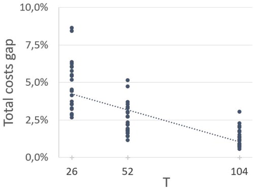
Figure 3. Costs difference as a function of failure probability.

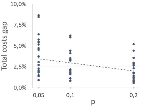
Figure 4. Costs difference as a function of the holding costs.

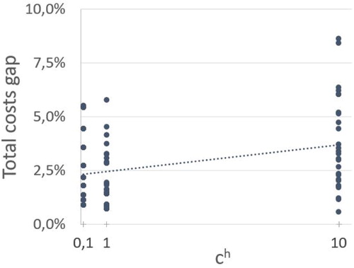
Table 3. Results of the regression analysis ($R^2=0.78$).

	T	$K^{\text{obj}}$	p	$c^{\mathrm{h}}$
Coefficient	$-4.4e^{-4}$	$-9.8e^{-2}$	$-1.9e^{-2}$	$1.4e^{-3}$
P-value	$5.5e^{-22}$	0.24	$2.6e^{-8}$	$1.4e^{-8}$

From the regression analysis, we learn that $c^{\mathrm{h}}$ has an impact on the mean costs difference. This is also clear from Figure 4. To understand how $c^{\mathrm{h}}$ affects the mean costs difference, we need to consider it in view of $c^{\mathrm{e}}$ and $c^{\mathrm{p}}.$ When $c^{\mathrm{h}}$ is one or more orders of magnitude lower than $c^{\mathrm{e}}$ and $c^{\mathrm{p}},$ both stocking policies will carry high inventories because having stock is much cheaper than having a shortage. As a result, the mean costs differences and the minimum and maximum gaps are similar when $c^{\mathrm{h}}=0.1$ and $c^{\mathrm{h}}=1,$ as Table 2 shows. The number of demands remaining until the end of the contract being in the state space, in the case of the flexible-time contract, a more adaptive stocking strategy can be followed if needed. As a result, the flexible-time contract has a strong end-of-horizon effect for expensive components ($c^{\mathrm{h}}=c^{\mathrm{e}}=10$). Given the high holding costs, every unit decrease of stock has a high impact on the total expected costs, resulting in a higher costs difference. The stronger end-of-horizon effect does not hurt the asset user. On average, the flexible-time contract results in 0.8% less XLDs than the fixed-time contract.

Table 4 gives an overview of the mean costs difference as a function of T and p. This table confirms that the mean costs difference decreases as T and p increase. A higher T and p give a higher pooling effect of the spare parts inventory being held in stock. When the contract covers more demand, an additional XLD can more easily be compensated by one of many other demands. Another explanation is that a higher T and p result in a lower coefficient of variation (CV) of the total demand realized during the fixed-time contract, as Table 4 shows.

Table A5. Detailed results of Section 7: Case 2.

	Mean costs			Mean XLDs
$p^{\text{true}}$	Fixed-time	Flexible-time	Gap(%)	Fixed-time	Flexible-time	Gap(%)
0.100	649.7	648.9	0.1	13.3	13.0	2.4
0.105	669.6	630.1	5.9	14.3	13.5	5.8
0.110	697.2	616.7	11.5	15.6	14.2	8.9
0.115	715.0	600.9	16.0	16.4	14.6	11.2
0.120	739.3	586.2	20.7	17.3	15.0	13.2
0.125	774.0	582.8	24.7	18.5	15.7	15.1

Table 4. Mean costs difference and cv depending on T and p.

	p
	0.05		0.1		0.2
T	Costs gap(%)	CV total demand	Costs gap(%)	CV total demand	Costs Gap(%)	CV total demand
26	6.0	0.156	4.7	0.107	3.5	0.071
52	3.2	0.111	2.4	0.076	1.8	0.051
104	1.6	0.078	1.3	0.053	0.9	0.036

5. Performance under an underestimated demand rate

As described in Section 1, providing an accurate estimation of the systems’ utilization level is challenging for asset users, and the estimate is often too low. This creates extra risk because the OEM will place less spare parts on stock than what is required for the true demand rate. This extra risk will hurt both the OEM and the asset user. The former risks paying high penalties, whereas the latter will be faced with more XLDs than expected, damaging its operations to an extent greater than the penalty can compensate for.

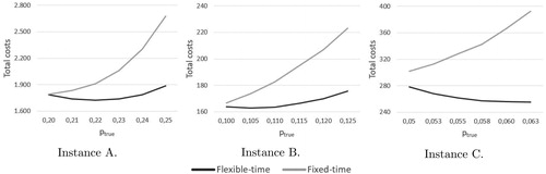
In this section, we compare the performance of the flexible-time contract with that of the fixed-time contract when the true demand rate deviates from the expected demand rate (the third research question). We consider not only the mean total costs and number of XLDs under both contracts, but also the deviation from their expected values based on the estimated demand rate. Our test bed consists of three instances summarized in Table 5. Instance A represents the instance yielding the smallest costs difference in Section 4. For instance B, we set all the parameters at the middle values of Table 1. Instance C is the one with the largest costs difference in Section 4.

Table 5. Instances used for the simulation under changing demand rate.

Instances	T	p	$K^{\text{obj}}$	$c^{\mathrm{h}}$	Gap(%)
A: Minimum costs difference	104	0.2	$3TNp/13=144$	10	0.6
B: Middle parameters	52	0.1	$2TNp/13=24$	1	1.6
C: Maximum costs difference	26	0.05	$3TNp/13=9$	10	8.6

In this section, we make use of simulation. Let λ denote the expected demand rate per machine, $\lambda =1/p.$ Let ${\lambda }^{\text{true}}$ denote the true demand rate during the contract execution phase. We define $p^{\text{true}}=1/{\lambda }^{\text{true}}.$ We focus our analysis on the realistic domain $p^{\text{true}}\ge p.$ We increase $p^{\text{true}}$ from p up to $1.25p,$ with increments of five percentage points; we then obtain integer values for F. For each instance, we generate random demand based on the binomial distribution with parameters $p^{\text{true}}$ and N. We refer to the generated demands for the whole contract duration as a demand sequence. For each instance, we simulate 100,000 demand sequences. We choose this high number to guarantee that the 95% confidence interval for the total costs has a width of, at most, 1% of the mean total costs. For the flexible-time contract, each demand sequence stops at the end of the first period for which the total demand is higher than or equal to F. For the fixed-time contract, each demand sequence stops after T periods. We compute the mean total costs associated with using the respective optimal inventory policies over the 100,000 simulated demand sequences, for each $p^{\text{true}}$ value, for both contracts. The detailed results for the three instances are available in Table A2 of the Appendix.

Figure 5 shows how the costs of both contracts evolve as the true demand rate increases. For all three instances and values of $p^{\text{true}},$ the fixed-time contract is more expensive than the flexible-time one. For instance A, the mean costs gap increases from only 0.6% when $p^{\text{true}}=p$ to 29.6% when $p^{\text{true}}=1.25p.$ For instances B and C, the gap increases from 1.6% to 21.3% and from 8.6% to 35.0%, respectively. These results indicate that the OEM can achieve significant savings when using a flexible-time contract, independent of the contract characteristics (i.e., duration and service level) and the spare part characteristics.

Figure 5. Impact of the true demand rate on the mean total costs.

In addition to the low mean costs under a flexible-time contract, the OEM is interested in the true costs being close to the expected costs to safeguard the profitability of the service contract. Under a flexible-time contract and for all instances, the costs for the OEM decrease when $p^{\text{true}}$ increases from p to $1.10p.$ When $p^{\text{true}}\ge 1.15p,$ the costs increase for instances A and B. The mean costs of the flexible-time contract are at most 6.7% higher than expected when $p^{\text{true}}=1.25p.$ For instance C, the costs are monotonically decreasing over the whole $p^{\text{true}}$ domain. By contrast, the mean costs of the fixed-time contract increase faster than $p^{\text{true}}$ for all instances and can be up to 49.3% higher than the expected costs when $p^{\text{true}}=1.25p.$

Two factors explain this difference between the two contracts: the stochastic duration of the flexible-time contract driving the majority of the costs difference and the end-of-horizon effect generating similar savings as in Section 4. We can assess the contribution of each factor by calculating the mean costs per demand using Table A2 of the Appendix. For the first factor, when $p^{\text{true}}\ge p,$ the flexible-time contract will end sooner than the fixed-time contract. The fixed-time contract runs until T periods, making the mean costs increase nonlinearly.

The second factor, the end-of-horizon effect, affects the inventory on-hand. For instances B and C, the mean inventory is lower and increases less under a flexible-time contract than under a fixed-time contract, as Table A2 shows. For instance A, this is also the case when $p^{\text{true}}=p$ up to $p^{\text{true}}=1.10p.$ When $p^{\text{true}}\ge 1.15p$ though, the inventory of the flexible-time contract is higher. By making use of U in the state-dependent base stock policy, the flexible-time contract is better able to take into the account the probability of exceeding $K^{\text{obj}}$ until the end of contract, resulting in lower costs. This is a direct consequence of the multimodularity properties, Theorem $1.\mathrm{A}.ix,$ and Theorem $1.\mathrm{B}.x,$ making the remaining allowed number of XLDs and the state-dependent base stock level economic substitutes.

The flexible-time contract also drives an improvement for the asset user. Figure 6 shows how the two contracts perform with respect to the XLD constraint. For instances A and B, the flexible-time contract results in a lower mean number of XLDs than the fixed-time contract. For instance C, however, the results are mixed, with the number of XLDs being higher for lower values of $p^{\text{true}}$ and lower for higher values of $p^{\text{true}}.$ For all instances though and for all $p^{\text{true}}$ values, the mean number of XLDs under a flexible-time contract remains lower than $K^{\text{obj}}.$ This is not the case for the fixed-time contract for instances A and C.

Figure 6. Impact of the true demand on the mean number of XLDs.

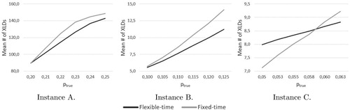
The mean number of XLDs resulting from the true demand deviates less from the expected number of XLDs under a flexible-time contract than under a fixed-time contract. Under the flexible-time contract, the realized mean number of XLDs can be up to 102.9% higher than expected as opposed to 148.2% for the fixed-time contract. The lower mean number of XLDs and the smaller difference between expected and realized mean number of XLDs are explained by the same two factors as the costs, that is, the stochastic duration of the flexible-time contract and the end-of-horizon effect.

6. Impact of updating the demand rate during the contract

In Section 5, we compared the performance of the flexible-time contract with the performance of the fixed-time contract when the true demand rate deviates from the expected demand rate. It is quite common in practice to update the estimated demand rate based on the observed demand during the contract execution phase. The updated estimated demand rate can then be used to update the base stock levels. In this section, we update the state-dependent base stock levels based on the observed demand rate, addressing the fourth research question.

Similar to Section 5, we focus our analysis on the realistic domain $p^{\text{true}}\ge p,$ and we simulate 100,000 demand sequences. The characteristically low demand rate for spare parts causes the OEM to notice a change in the demand rate relatively late in the contract. We update the demand rate halfway through the contract. For the flexible-time contract, halfway means the first decision epoch for which the realized demand is higher than or equal to $F/2.$ For the fixed-time contract, halfway means period $T/2.$

Let $p^{\text{observed}}$ denote the demand rate observed in the first half of the contract. We define $p^{\text{updated}}=(1-\alpha )p+\alpha p^{\text{observed}},\alpha \in \{0.0,0.25,0.5\},$ where α = 0 corresponds to no updating. For both contracts, the state-dependent base stock levels are updated using $p^{\text{updated}}.$ With each MDP being CPU-bounded, this step is computationally expensive. Therefore, we reduce the test bed by focusing on one instance. To obtain conservative results in favor of the fixed-time contract, we choose an instance with a low mean costs difference. Instance A used in Section 5 has the lowest mean costs difference, but a very large state space. Two instances have the second lowest mean costs difference of 0.8%. We choose the one with the smallest state space, resulting in a 10-fold decrease in the state space size. This instance is the instance with T = 104, p = 0.1, $K^{\text{obj}}=F/13=24,$ and $c^{\mathrm{h}}=1.$ Last, we consider three values of $p^{\text{true}}:$ 0.1, 0.1125, and 0.125. We choose these values because they are close to the settings of Section 5. Having three values for $p^{\text{true}}$ and three values for α, our test bed yields nine instances. We compute the mean total costs associated with using the respective optimal inventory policies over the 100 000 simulated demand sequences for both contracts. Table A3 in the Appendix provides detailed results. The flexible-time contract results in lower costs and less XLDs for all instances.

To reduce the mean costs and the mean number of XLDs, the OEM and the asset user have three options when taking a fixed-time contract without updating as starting point. First, they can decide to keep a fixed-time contract and update the demand rate during the contract execution phase. Second, they can decide to use a non-updated flexible-time contract. Third, they can agree on using an updated flexible-time contract. To compare these alternatives, we focus on the setting with $p^{\text{true}}=0.125$ and $\alpha =0.5.$ Figures 7 and 8 show how the mean costs and the mean number of XLDs decrease depending on the path chosen by the OEM and the asset user.

Figure 7. Reduction of mean costs.

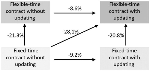
Figure 8. Reduction of mean number of XLDs.

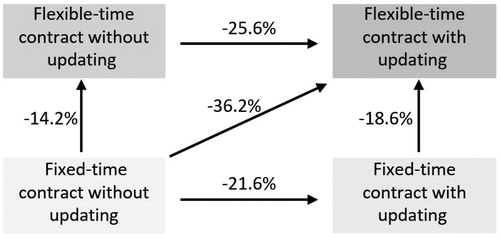
Moving from a non-updated fixed-time contract to an non-updated flexible-time contract leads to a higher costs decrease than moving to an updated fixed-term contract. As the OEM can only observe the actual demand rate late during the contract execution phase, the mean costs decrease remains limited when updating the demand rate. The improvement brought by updating the demand rate helps the OEM only in the second half of the contract. The OEM might have incurred high costs already in the first half of the contract. Updating the demand rate allows for a direct adjustment of the state-dependent base stock levels. The OEM would thus increase the inventory to compensate for the increased risk of exceeding $K^{\text{obj}}$ and incurring potential (additional) penalty costs. The updated state-dependent base stock policy has a high impact on the reduction of the mean number of XLDs. For the asset user, updating the demand rate brings the most benefits.

7. Extension to a multi-item setting

In this section, we answer our fifth research question. We compare the performance of the flexible-time contract with the fixed-time contract for multiple components (fifth research question). We derive the multi-item optimal policy for both contracts and use simulation to extend the insights of Section 5 to a multi-item setting. The detailed MDP formulations for both contracts are available in the supplemental online material.

Given the computational complexity, we set N = 5 and consider two Stock-Keeping Units (SKUs). We draw on instance B to define the characteristics of each SKU. We chose instance B because all variables are set at their middle value and the mean costs gap is lower than the mean costs gap of the total test bed used in Section 4. Choosing this instance leads to results that are conservative in favor of the fixed-time contract. We define two cases for which we set the values as shown in Table 6. Case 1 represents two SKUs with the same reliability and the same price. Case 2 represents a mix of a reliable, expensive SKU and a cheaper, less reliable SKU.

Table 6. Multi-item cases.

	F	$K^{\text{obj}}$	p1	p2	$c_1^{\mathrm{h}}$	$c_2^{\mathrm{h}}$
Case 1	52Np	$2F/13$	0.05	0.05	1	1
Case 2	52Np	$2F/13$	0.01	0.09	1.8	0.2

We compare the performance of the flexible-time and fixed-time contracts by using the multi-item optimal policies for both contracts in a simulation model. We build the simulation in a similar way to that in Section 5. The detailed results are available in the Appendix, Tables A4 and A5 for Cases 1 and 2, respectively. Tables 7 and 8 show how the results of Section 5 extend to a multi-item setting with respect to the mean costs and mean number of XLDs, respectively.

Table 7. Impact of the multi-item setting on the mean costs gap.

	Mean costs gap(%)
$p^{\text{true}}$	Single-item	Case 1	Case 2
0.100	1.6	1.0	0.1
0.105	6.3	7.5	5.9
0.110	10.6	13.0	11.5
0.115	14.7	18.0	16.0
0.120	17.9	22.7	20.7
0.125	21.3	26.6	24.7

Table 8. Impact of the multi-item setting on the mean XLD gap.

	Mean XLD gap(%)
$p^{\text{true}}$	Single-item	Case 1	Case 2
0.100	2.8	1.9	2.4
0.105	7.3	1.1	5.8
0.110	11.1	3.2	8.9
0.150	15.1	4.5	11.2
0.120	18.0	5.8	13.2
0.125	20.6	7.0	15.1

In a multi-item setting, a pooling effect occurs across the two items. The availability of one component can compensate for the non-availability of another. We observe that the mean costs difference is somewhat higher in the multi-item setting, but the mean XLD difference is lower than in the single-item model. The flexible-time contract remains beneficial to both the OEM and the asset user. It results in lower mean costs and less XLDs. We conclude that the main findings of the single-item model also hold in a multi-item setting.

8. Conclusion

OEMs estimate the costs of executing a service contract based on the expected demand rate derived from an estimated utilization level provided by the asset user. During the contract execution phase and under an accurate estimation of the utilization level, the low demand rate of spare parts combined with the finite horizon of fixed-time contracts brings a high costs uncertainty. This effect is exacerbated because estimating the utilization level is a challenging task for asset users, who prefer to provide conservative values to the OEM.

We proposed an alternative approach to reduce the risks associated with service contract delivery. We introduced the flexible-time contract, defined over an agreed-on number of spare parts demands. We examined the optimal inventory policy and proved that its structure is a state-dependent base stock policy. We compared the optimal expected costs of the flexible-time contract with those of a fixed-time contract over a large test bed. Under an accurate demand rate estimation, the flexible-time contract results in up to 8.6% savings for the OEM. The savings increase as the reliability of the components increases and the contract duration decreases. Using the state-dependent base stock policy in a simulation, we assessed how the two contracts compare when the demand rate is underestimated in the contracting phase. In this setting, the flexible-time contract results in significantly lower mean costs and mean number of XLDs. When the true demand rate is 25% higher than the estimated demand rate, the flexible-time contract is up to 35% cheaper and never exceeds the agreed-on number of XLDs. Demand rate updating is a common way to adjust base stock levels during the contract execution phase. We extended our simulation by updating the demand rate forecast during the contract and adjusting the inventory policy. Both contracts benefit almost equally from updating the demand rate. When extending our model to a multi-item setting, the main findings remain unchanged. Two main factors make the flexible-time contract perform better than the fixed-time contract for both the OEM and the asset user. First, the stochastic duration of the flexible-time contract enables the contract to end sooner when the true demand rate is higher than expected. Second, the flexible-time contract makes a direct connection between the remaining contract coverage and the allowed late deliveries.

The flexible-time contract has a variable time duration. Its implementation in practice should be supported by a review process between the OEM and the asset user. In the review process, the two parties would review the performance as well as a potential deviation of the observed demand rate from the estimated demand rate. Often in practice, the OEM and the asset user have regular performance review meetings. The time between these meetings is always shorter than the contract duration. For example, it is common for a service contract of a high-tech system to be established for a 3-year period while review meetings occur on a monthly basis. Adding the observed demand rate as a metric in these meetings would be necessary to trigger the contract renewal on time.

Acknowledgments

The authors thank the associate editor and the reviewers for the valuable comments, which helped to improve the quality of the paper.

Additional information

Notes on contributors

Douniel Lamghari-Idrissi

Douniel Lamghari-Idrissi is a part-time PhD candidate at the school of Industrial Engineering at Eindhoven University of Technology. His current research topic is the design of after sales services that lead to more stable operations for the asset users. He worked almost a decade in the pharmaceutical industry, holding various functions from sustainability to supply chain management. He joined ASML Netherlands B.V. in 2013, in customer supply chain management. As program manager, he develops and implements solutions to help chip-makers in their operations.

Rob Basten

Rob Basten is an associate professor at Eindhoven University of Technology (TU/e) where he is primarily occupied with after sales services for high-tech equipment. He is especially interested in using new technologies to improve after sales services. For example, 3D printing of spare parts on location and using improved sensoring and communication technology to perform “just in time” maintenance. He is further active in behavioral operations management, trying to understand how people can use decision support systems in such a way that they actually improve decisions and add value. Many research projects are interdisciplinary in order to carry out high quality research and solve real life problems in cooperation with high-tech companies such as ASML.

Geert-Jan van Houtum

Geert-Jan van Houtum is a professor of maintenance and reliability at the Department of Industrial Engineering and Innovation Sciences, Eindhoven University of Technology. His research is focused on predictive maintenance, availability management of capital goods, spare parts management, and the effect of design decisions on the total cost of ownership of capital goods. Much of his research is based on a close collaboration with e.g., ASML, Dutch Railways, Lely, Philips, and the Royal Netherlands Navy. He is associate editor at Manufacturing and Service Operations Management and area editor at Service Science.

Appendix A.

Detailed computational results

Table A1. Detailed results of Section 4.

				Fixed-time		Flexible-time		Costs
p	T	$K^{\text{obj}}$	$c_{\mathrm{h}}$	Costs	Mean I	Costs	Mean I	gap(%)
0.05	26	$\mathit{TNp}/13$	0.1	10.2	5.0	9.6	4.8	5.5
0.05	26	$\mathit{TNp}/13$	1	70.2	3.6	66.2	3.4	5.8
0.05	26	$\mathit{TNp}/13$	10	456.8	2.8	427.7	2.7	6.4
0.05	26	$2TNp/13$	0.1	10.1	5.0	9.6	4.7	5.4
0.05	26	$2TNp/13$	1	63.1	3.1	60.2	3.0	4.5
0.05	26	$2TNp/13$	10	360.4	2.4	330.0	2.2	8.4
0.05	26	$3TNp/13$	0.1	10.1	5.0	9.6	4.7	5.4
0.05	26	$3TNp/13$	1	62.1	3.0	59.8	2.9	3.7
0.05	26	$3TNp/13$	10	300.2	2.1	274.3	1.9	8.6
0.1	26	$\mathit{TNp}/13$	0.1	13.1	7.0	12.6	6.7	4.4
0.1	26	$\mathit{TNp}/13$	1	86.1	5.3	82.6	5.1	4.1
0.1	26	$\mathit{TNp}/13$	10	535.4	4.4	503.1	4.3	6.0
0.1	26	$2TNp/13$	0.1	13.1	7.0	12.5	6.7	4.4
0.1	26	$2TNp/13$	1	83.3	5.0	80.6	4.9	3.3
0.1	26	$2TNp/13$	10	412.2	3.8	386.6	3.6	6.2
0.1	26	$3TNp/13$	0.1	13.1	7.0	12.5	6.7	4.4
0.1	26	$3TNp/13$	1	83.3	5.0	80.6	4.9	3.2
0.1	26	$3TNp/13$	10	362.4	3.3	340.5	3.1	6.0
0.2	26	$\mathit{TNp}/13$	0.1	16.6	11.0	16.0	10.7	3.5
0.2	26	$\mathit{TNp}/13$	1	106.9	9.0	103.8	8.8	2.9
0.2	26	$\mathit{TNp}/13$	10	592.8	7.4	562.1	7.2	5.2
0.2	26	$2TNp/13$	0.1	16.6	11.0	16.0	10.7	3.5
0.2	26	$2TNp/13$	1	106.7	9.0	103.7	8.8	2.8
0.2	26	$2TNp/13$	10	479.2	6.4	458.0	6.2	4.4
0.2	26	$3TNp/13$	0.1	16.6	11.0	16.0	10.7	3.5
0.2	26	$3TNp/13$	1	106.7	9.0	103.7	8.8	2.8
0.2	26	$3TNp/13$	10	450.4	6.0	438.4	5.9	2.6
0.05	52	$\mathit{TNp}/13$	0.1	20.3	5.0	19.7	4.9	2.7
0.05	52	$\mathit{TNp}/13$	1	131.0	3.3	127.0	3.2	3.1
0.05	52	$\mathit{TNp}/13$	10	867.6	2.8	835.5	2.8	3.7
0.05	52	$2TNp/13$	0.1	20.3	5.0	19.7	4.9	2.7
0.05	52	$2TNp/13$	1	124.2	3.0	121.8	3.0	1.9
0.05	52	$2TNp/13$	10	672.1	2.3	637.5	2.2	5.1
0.05	52	$3TNp/13$	0.1	20.3	5.0	19.7	4.9	2.7
0.05	52	$3TNp/13$	1	124.0	3.0	121.7	3.0	1.8
0.05	52	$3TNp/13$	10	562.9	2.0	536.3	1.9	4.7
0.1	52	$\mathit{TNp}/13$	0.1	26.2	7.0	25.7	6.9	2.2
0.1	52	$\mathit{TNp}/13$	1	167.7	5.1	164.6	5.0	1.9
0.1	52	$\mathit{TNp}/13$	10	1008.0	4.4	972.3	4.3	3.5
0.1	52	$2TNp/13$	0.1	26.2	7.0	25.7	6.9	2.2
0.1	52	$2TNp/13$	1	166.6	5.0	163.9	4.9	1.6
0.1	52	$2TNp/13$	10	783.4	3.7	757.0	3.6	3.4
0.1	52	$3TNp/13$	0.1	26.2	7.0	25.7	6.9	2.2
0.1	52	$3TNp/13$	1	166.6	5.0	163.9	4.9	1.6
0.1	52	$3TNp/13$	10	694.7	3.2	672.0	3.1	3.3
0.2	52	$\mathit{TNp}/13$	0.1	33.3	11.0	32.7	10.8	1.8
0.2	52	$\mathit{TNp}/13$	1	213.5	9.0	210.5	8.9	1.4
0.2	52	$\mathit{TNp}/13$	10	1118.4	7.3	1085.2	7.1	3.0
0.2	52	$2TNp/13$	0.1	33.3	11.0	32.7	10.8	1.8
0.2	52	$2TNp/13$	1	213.5	9.0	210.5	8.9	1.4
0.2	52	$2TNp/13$	10	927.9	6.2	906.3	6.1	2.3
0.2	52	$3TNp/13$	0.1	33.3	11.0	32.7	10.8	1.8
0.2	52	$3TNp/13$	1	213.5	9.0	210.5	8.9	1.4
0.2	52	$3TNp/13$	10	896.2	6.0	886.0	5.9	1.1
0.05	104	$\mathit{TNp}/13$	0.1	40.6	5.0	40.0	4.9	1.4
0.05	104	$\mathit{TNp}/13$	1	253.1	3.1	249.4	3.1	1.5
0.05	104	$\mathit{TNp}/13$	10	1676.0	2.8	1641.1	2.8	2.1
0.05	104	$2TNp/13$	0.1	40.6	5.0	40.0	4.9	1.4
0.05	104	$2TNp/13$	1	247.9	3.0	245.7	3.0	0.9
0.05	104	$2TNp/13$	10	1283.4	2.3	1244.3	2.2	3.0
0.05	104	$3TNp/13$	0.1	40.6	5.0	40.0	4.9	1.4
0.05	104	$3TNp/13$	1	247.9	3.0	245.7	3.0	0.9
0.05	104	$3TNp/13$	10	1086.1	1.9	1061.4	1.9	2.3
0.1	104	$\mathit{TNp}/13$	0.1	52.5	7.0	51.9	6.9	1.1
0.1	104	$\mathit{TNp}/13$	1	333.4	5.0	330.6	5.0	0.8
0.1	104	$\mathit{TNp}/13$	10	1937.5	4.4	1898.4	4.3	2.0
0.1	104	$2TNp/13$	0.1	52.5	7.0	51.9	6.9	1.1
0.1	104	$2TNp/13$	1	333.1	5.0	330.4	5.0	0.8
0.1	104	$2TNp/13$	10	1523.6	3.6	1496.6	3.5	1.8
0.1	104	$3TNp/13$	0.1	52.5	7.0	51.9	6.9	1.1
0.1	104	$3TNp/13$	1	333.1	5.0	330.4	5.0	0.8
0.1	104	$3TNp/13$	10	1357.1	3.1	1333.4	3.0	1.7
0.2	104	$\mathit{TNp}/13$	0.1	66.5	11.0	65.9	10.9	0.9
0.2	104	$\mathit{TNp}/13$	1	427.0	9.0	424.0	8.9	0.7
0.2	104	$\mathit{TNp}/13$	10	2155.3	7.2	2118.7	7.1	1.7
0.2	104	$2TNp/13$	0.1	66.5	11.0	65.9	10.9	0.9
0.2	104	$2TNp/13$	1	427.0	9.0	424.0	8.9	0.7
0.2	104	$2TNp/13$	10	1823.4	6.1	1801.3	6.0	1.2
0.2	104	$3TNp/13$	0.1	66.5	11.0	65.9	10.9	0.9
0.2	104	$3TNp/13$	1	427.0	9.0	424.0	8.9	0.7
0.2	104	$3TNp/13$	10	1791.7	6.0	1781.8	6.0	0.6

Table A2. Detailed results of Section 5.

		Mean Costs		Mean # of XLDs		Mean duration		Mean demand		Mean inventory
$p^{\text{true}}$		Flexible-time	Fixed- time	Flexible-time	Fixed-time	Flexible-time	Fixed-time	Flexible-time	Fixed-time	Flexible-time	Fixed-time
Instance A	0.200	1782.7	1793.2	89.42	89.67	104.5	104.0	624.0	624.0	11.27	13.98
	0.210	1738.2	1833.3	101.97	107.34	99.5	104.0	624.0	655.6	11.58	14.82
	0.220	1723.5	1910.4	114.33	124.75	95.1	104.0	624.0	686.3	11.89	14.01
	0.230	1738.7	2058.7	126.69	138.24	90.9	104.0	624.0	717.6	11.24	9.10
	0.240	1787.9	2301.4	136.88	144.66	87.2	104.0	624.0	748.8	8.59	4.93
	0.250	1886.8	2678.7	142.95	148.53	83.7	104.0	624.0	779.9	4.97	4.81
Instance B	0.100	163.9	166.5	5.54	5.70	52.4	52.0	156.0	156.1	2.91	3.19
	0.105	162.7	173.6	6.52	7.03	50.0	52.0	156.0	163.7	3.19	3.60
	0.110	163.3	182.7	7.61	8.56	47.7	52.0	156.0	171.6	3.38	3.93
	0.115	166.2	194.8	8.81	10.38	45.7	52.0	156.0	179.6	3.65	4.38
	0.120	169.9	207.0	9.94	12.12	43.9	52.0	156.0	187.0	3.83	4.61
	0.125	175.7	223.2	11.24	14.15	42.1	52.0	156.0	195.0	4.11	4.85
Instance C	0.050	275.3	301.7	7.99	7.13	26.5	26.0	39.0	38.9	1.09	1.85
	0.053	268.1	312.6	8.18	7.59	25.2	26.0	39.0	41.0	1.09	1.89
	0.055	261.6	328.0	8.34	8.01	24.1	26.0	39.0	43.1	1.09	1.91
	0.058	256.9	342.8	8.49	8.37	23.1	26.0	39.0	44.8	1.09	1.90
	0.060	255.7	366.1	8.67	8.83	22.2	27.0	39.0	46.8	1.11	1.93
	0.063	255.3	392.7	8.82	9.22	21.4	26.0	39.0	48.6	1.14	2.05

Table A3. Detailed results of Section 6.

		Mean Costs		Mean # of XLDs		Mean duration		Mean demand		Mean inventory
$p^{\text{true}}$	α	Flexible-time	Fixed-time	Flexible-time	Fixed-time	Flexible-time	Fixed-time	Flexible-time	Fixed-time	Flexible-time	Fixed-time
0.1000	0.00	330.5	333.0	11.2	11.4	104.5	104.0	312.0	312.0	4.97	5.00
	$0.25$	330.5	333.0	$11.2$	$11.4$	$104.5$	104.0	312.0	312.0	$4.97$	5.00
	$0.50$	331.2	333.7	$10.9$	$11.1$	$104.5$	104.0	312.0	312.0	$5.00$	5.03
0.1125	$0.00$	330.8	375.6	$16.4$	$18.6$	$92.9$	104.0	312.0	351.1	$4.97$	5.02
	$0.25$	329.3	374.0	$15.8$	$18.0$	$92.9$	104.0	312.0	351.1	$5.03$	5.06
	$0.50$	324.6	368.4	$13.7$	$15.6$	92.9	104.0	312.0	351.1	$5.23$	5.27
0.1250	$0.00$	354.2	450.1	$22.2$	$25.9$	$83.7$	104.0	312.0	390.0	$5.01$	5.19
	$0.25$	334.9	422.4	$18.8$	$22.8$	$83.7$	104.0	312.0	390.0	$5.26$	5.37
	$0.50$	323.7	408.7	$16.5$	$20.3$	$83.7$	104.0	312.0	390.0	$5.42$	5.51

Table A4. Detailed results of Section 7: Case 1.

	Mean costs			Mean XLDs
$p^{\text{true}}$	Fixed-time	Flexible-time	Gap(%)	Fixed-time	Flexible-time	Gap(%)
0.100	714.1	706.8	1.0	18.2	17.9	1.9
0.105	751.2	695.2	7.5	18.9	18.7	1.1
0.110	787.6	685.3	13.0	19.8	19.1	3.2
0.115	836.7	686.4	18.0	20.8	19.8	4.5
0.120	881.9	681.9	22.7	21.5	20.3	5.8
0.125	936.2	686.7	26.6	22.4	20.8	7.0

References

- Cohen, M.A. and Agrawal, N. (1999) An analytical comparison of long and short term contracts. IIE Transactions, 31(8), 783–796.
- Fahimnia, B., Tang, C.S., Davarzani, H. and Sarkis, J. (2015) Quantitative models for managing supply chain risks: A review. European Journal of Operational Research, 247(1), 1–15.
- Gebauer, H., Saul, C.J., Haldimann, M. and Gustafsson, A. (2017) Organizational capabilities for pay-per-use services in product-oriented companies. International Journal of Production Economics, 192, 157–168.
- Geng, N. and Jiang, Z. (2009) A review on strategic capacity planning for the semiconductor manufacturing industry. International Journal of Production Research, 47(13), 3639–3655.
- Gerchak, Y. and He, Q.M. (2003) On the relation between the benefits of risk pooling and the variability of demand. IIE Transactions, 35(11), 1027–1031.
- Hishamuddin, H., Sarker, R. and Essam, D. (2012) A disruption recovery model for a single stage production-inventory system. European Journal of Operational Research, 222(3), 464–473.
- Hopp, W. and Spearman, M. (2011) Factory Physics, third edition, Waveland Press, Long Grove, Illinois.
- Hu, Q., Boylan, J.E., Chen, H. and Labib, A. (2018) OR in spare parts management: A review. European Journal of Operational Research, 266(2), 395–414.
- Hyvönen, T. and Järvinen, J. (2006) Contract-based budgeting in health care: A study of the institutional processes of accounting change. European Accounting Review, 15(1), 3–36.
- Kim, B. and Park, S. (2008) Optimal pricing, EOL (end of life) warranty, and spare parts manufacturing strategy amid product transition. European Journal of Operational Research, 188(3), 723–745.
- Kim, S.H., Cohen, M.A., Netessine, S. and Veeraraghavan, S. (2010) Contracting for infrequent restoration and recovery of mission-critical systems. Management Science, 56(9), 1551–1567.
- Koch, B.S., Mayper, A.G. and Wilner, N.A. (2009) The interaction of accountability and post-completion audits on capital budgeting decisions. Academy of Accounting and Financial Studies Journal, 13, 1–26.
- Koole, G. (2007) Monotonicity in Markov reward and decision chains: Theory and applications. Foundations and Trends® in Stochastic Systems, 1(1), 1–76.
- Lamghari-Idrissi, D., Basten, R., Dellaert, N. and van Houtum, G.J. (2020) Which spare parts service measure to choose for a front-end wafer fab? IEEE Transactions on Semiconductor Manufacturing, 33(4), 504–510.
- Lamghari-Idrissi, D., Basten, R. and van Houtum, G.J. (2020) Spare parts inventory control under a fixed-term contract with a long-down constraint. International Journal of Production Economics, 219, 123–137.
- Li, Q. and Yu, P. (2014) Multimodularity and its applications in three stochastic dynamic inventory problems. Manufacturing & Service Operations Management, 16(3), 455–463.
- Mak, H.Y. and Shen, Z.J.M. (2012) Risk diversification and risk pooling in supply chain design. IIE Transactions, 44(8), 603–621.
- Mönch, L., Uzsoy, R. and Fowler, J.W. (2018) A survey of semiconductor supply chain models part i: Semiconductor supply chains, strategic network design, and supply chain simulation. International Journal of Production Research, 56(13), 4524–4545.
- Pascual, R., Santelices, G., Liao, H. and Maturana, S. (2016) Channel coordination on fixed-term maintenance outsourcing contracts. IIE Transactions, 48(7), 651–660.
- Song, J.S., van Houtum, G.J. and van Mieghem, J.A. (2020) Capacity and inventory management: Review, trends, and projections. Manufacturing & Service Operations Management, 22(1), 36–46.
- Tan, Y.R., Paul, A.A., Deng, Q. and Wei, L. (2017) Mitigating inventory overstocking: Optimal order-up-to level to achieve a target fill rate over a finite horizon. Production and Operations Management, 26(11), 1971–1988.
- Van Der Auweraer, S., Boute, R.N. and Syntetos, A.A. (2019) Forecasting spare part demand with installed base information: A review. International Journal of Forecasting, 35(1), 181–196.
- Visnjic, I., Jovanovic, M., Neely, A. and Engwall, M. (2017) What brings the value to outcome-based contract providers? Value drivers in outcome business models. International Journal of Production Economics, 192, 169–181.