Virtual sensing network for statistical process monitoring

Abstract

Physical sensing is increasingly implemented in modern industries to improve information visibility, which generates real-time signals that are spatially distributed and temporally varying. These signals are often nonlinear and nonstationary in the high-dimensional space, which pose significant challenges to monitoring and control of complex systems. Therefore, this article presents a new “virtual sensing” approach that places imaginary sensors at different locations in signaling trajectories to monitor evolving dynamics within the signal space. First, we propose self-organizing principles to investigate distributional and topological features of nonlinear signals for optimal placement of imaginary sensors. Second, we design and develop the network model to represent real-time flux dynamics among these virtual sensors, in which each node represents a virtual sensor, while edges signify signal flux among sensors. Third, the establishment of a network model as well as the notion of transition uncertainty enable a fine-grained view into system dynamics and then extend a new Flux Rank (FR) algorithm for process monitoring. Experimental results show that the network FR methodology not only delineate real-time flux patterns in nonlinear signals, but also effectively monitor spatiotemporal changes in the dynamics of nonlinear dynamical systems.

Keywords:

• Virtual sensing
• network model
• flux rank
• self-organization
• general likelihood ratio
• statistical process control

1. Introduction

Physical sensors are increasingly deployed in modern industries to improve information visibility for monitoring and control of complex systems. As a result, multidimensional sensor signals are accumulated at high velocity, resulting in a high data volume. There is an urgent need to process and analyze these signals for a myriad of purposes, such as condition monitoring, anomaly detection, and quality improvements. However, these signals are different from traditional quality features (e.g., geometric measurements or defect quantities of products) that can directly apply Statistical Process Control (SPC) methods. Rather, it is common that sensor signals are nonlinear and nonstationary in the high-dimensional space, which pose significant challenges to conventional statistical monitoring techniques.

Virtual sensing entails the processing and transformation of nonlinear signals using a model or transfer function. This, in turn, enables a fine-grained examination into system dynamics and further extracts useful information for change detection in the undercurrents of nonlinear dynamical systems. Virtual Sensors (VSs) can be used alongside or in lieu of physical sensors to mitigate practical or analytical constraints in the real world. Nonetheless, the notion of virtual sensing is rather broad, because the scope of transformation modeling is large. In this investigation, we focus on virtual sensing within the context of placing sensors at different locations of signaling trajectories to monitor evolving dynamics within the signal space. In this regard, VS can be treated as imaginary sensors that sense the flux dynamics of signals, also referred to as virtual flux sensing.

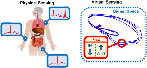
As illustrated in Figure 1, physical sensing places “real” sensors at different locations of a complex system and then records operational dynamics or physical activity as time-varying signals. For example, ElectroCardioGram (ECG) signals are observed with electrical sensors attached to the body surface, which capture operational dynamics of the human heart from different perspectives. A traditional 12-lead ECG examines electrical activity from 12 different angles around the heart, whereas a three-lead Vector Cardio Gram (VCG) is from three orthogonal directions. See more details about ECG sensing systems in Yang et al. (2012). Real-time sensor signals are often spatiotemporally varying in the high-dimensional space. On the other hand, virtual sensing places “imaginary” sensors at different locations of signaling trajectories that focus more on the influx and outflux dynamics in a small neighborhood of a VS. In fact, there are practical constraints in the use of physical sensors to directly observe such minute details. Virtual sensing offers an unparalleled advantage to take a closer look into operational dynamics of a complex system.

Figure 1. A physical sensing system (left) where physical sensors are distributionally placed on the human body. The physical sensing system is compared against a virtual flux sensing system (right) where VSs placed in the signal space generate influx and outflux readings based on nearby signals.

SPC techniques are widely used in the manufacturing industry for quality control applications. However, very little has been done to investigate virtual sensing and pertinent applications for sensor-based process monitoring and control. The current article presents a virtual sensing approach for monitoring real-time flux dynamics in nonlinear signals and detecting the changes in the dynamics of nonlinear systems. VSs are treated as nodes to transform the signals into a network, which necessitates an effective way of relating constituent components to one another. Network theory provides a promising avenue to characterize and model signal streams obtained from nonlinear dynamical systems. To this end, a collection of VSs can be converted into a network structure by representing sensors as nodes and flux dynamics as the weights of edges. Statistical process monitoring can then focus on the networking behaviors of both nodes and edges, which reveal individual and interactive characteristics in the underlying operations, respectively. Specifically, our contributions are summarized as follows:

1. Self-organizing virtual sensing: Placement of VSs within the signal space is the first problem that needs to be solved. We propose to leverage self-organizing principles to investigate distributional and topological features of nonlinear signals for optimal placement of anchoring sensors. As such, virtual sensors will learn topological structures and then self-organize within the signal space. Each sensor will sense the flux dynamics in a spatiotemporal neighborhood along the signaling trajectory.

2. VS network modeling and flux rank: Further, we develop a network model to represent and model real-time flux dynamics among these VSs, in which each node represents a VS, while edges are signal flux among sensors. A new Flux Rank (FR) algorithm is also designed to characterize and quantify influx and outflux transition dynamics around each sensor.

3. FR SPC: It is worth noting that FR statistics are compositional, where constituent elements sum to one. Hence, we designed new FR control charts, namely FR ${\chi }^2,$ Hotelling $T^2,$ and General Likelihood Ratio charts, for detecting the changes in the flux dynamics of nonlinear signals, thereby monitoring nonlinear dynamical systems.

The proposed virtual sensing approach is evaluated and validated with case studies on nonlinear Lorenz systems, as well as physiological signals. Experimental results show that a VS network and FR SPC algorithms not only delineate real-time flux patterns in nonlinear signals, but also effectively monitor spatiotemporal changes in the dynamics of nonlinear systems. The proposed VS-based monitoring approach shows great potential as a SPC technique for monitoring multidimensional nonlinear signals from complex systems.

The remainder of this article is organized as follows: Section 2 provides a review of virtual measurement, network modeling and representation, as well as SPC and network monitoring. Section 3 presents the research methodology of virtual sensing networks and the FR monitoring. Section 4 introduces case studies and the design of benchmark experiments. Section 5 presents experimental results and discusses broader implications of virtual sensing approaches. Section 6 includes the conclusions from this investigation and summarizes the niches filled by virtual sensing.

2. Research background

2.1. Virtual measurement

Generation of virtual measurements has ambiguous connotations. Various techniques bear the moniker “virtual”. For example, virtual metrology typically refers to a set of methods employed to predict the surface properties of a silicon wafer without direct measurements (e.g., atomic force microscope, X-ray), but rather through predicted conjectures from machine parameters, process information, and in-situ sensor signals (Cheng et al., 2012; Hsieh et al., 2019; Yang, Blue, Roussy, Pinaton and Reis, 2020). On the other hand, soft sensing generally refers to an estimation model that integrates available measurements and system knowledge to predict a quantity that cannot or need not be measured (Lin et al., 2007). Examples of soft sensing implementations include the well-known Kalman filter or neural network. Soft sensors have also been deployed to monitor chemical processes through the utilization of statistical tools such as feature extraction methods and SPC principles (Fortuna et al., 2007; Masuda et al., 2014; Funatsu, 2018). In the literature, either virtual metrology or soft sensing refers to the use of signals (i.e., can be readily measured) or knowledge (e.g., existing models or domain-specific information) to predict measurement quantities that are difficult to be directly measured.

Placement of “imaginary” sensors in the signal space (what we refer to as VSs) should conform to a signal’s topology. More sensors should be deployed in spatial regions where signals are denser to provide higher sensing resolution. Likewise, regions where signal presence is sparse would require less virtual sensing capability. Spatial indexing techniques may offer one solution to the problem of VS placement. Typically, these indexing techniques utilize hypercube geometries to represent their regions (Kim and Patel, 2010). Chen and Yang (2016) develop quadtree partitioning to represent a spatiotemporal signal as a discrete state timeseries. Analyzing the heterogeneous recurrence dynamics of this discrete state timeseries with fractal analysis allowed for the monitoring of nonlinear dynamic systems including autoregressive processes, Lorenz processes, ultra-precision machining signals, and VCG signals. Similarly, Cheng et al. (2016) cultivate heterogeneous recurrence methods to assist in the identification of patients suffering from obstructive sleep apnea utilizing ECG signals. Self-organizing methods may also be employed in the determination of network topology and, therefore, inform VS spatial placement. Liu and Yang (2018) employ a “charged-particle” self-organization scheme for the purposes of variable clustering. Input variables are grouped via nonlinear coupling, which leverages cross recurrences between two variables. Reducing the amount of redundant information yields higher-quality predictive analytics. Similarly, Yang, Liu and Kumara (2020) designed a self-organization approach to reconstruct the topologies of voxelized 3D objects from the network adjacency matrix. Simply storing the adjacency matrix aids in the search and reuse of engineering designs as this network feature is vastly less complex than the CAD models.

Given the literature surveyed, we have identified the following gaps:

1. There is little mention of placing VSs within the signal space. Measurements derived from VSs placed within the signal space provides an unprecedented opportunity for the extraction of a unique set of patterns in a nonlinear signal. Nonetheless, the optimal way to handle VS placement is a pertinent gap to this investigation.

2. The existing practice of spatial indexing does not take full advantage of the nonlinear geometry of signal space and is often limited in representing the regions of VSs. The hypercubic shape of the partitioning scheme may generate sensing regions for signal outliers, even where signals are dense.

3. Self-organization has yet to be explored to sufficient capacity in the domain of VS placement. Signal topology plays a critical role in statistical monitoring of system dynamics.

2.2. Network science

Once VSs are placed, they will produce new sets of inflow and outflow signals. Network science offers the ability to study the output of the VSs. Representing a system as a network is a crucial first step in this domain. One must determine which features in a system are analogous to network nodes and edges. For example, Sadreazami et al. (2018) represent each sensor in their blind intrusion detection system as a node. Nodes are connected by edges if they are within a certain geographic radius to one another. Once the representation is established, the system may be converted into a network. Nonetheless, there are cases where a network’s topology is unknown. Zhang et al. (2021) develop a structure identification methodology. The method can determine a temporally evolving network topology in situations where sparse and noisy signals are present. Such structure identification allows for the monitoring of complex industrial cyber-physical systems.

Papadimitriou et al. (2010) developed a set of network similarity-based approaches to detect anomalies in web graphs over time. In addition to vertices and edges, each graph considers the PageRank as a critical feature. Potential anomalies in a web graph are defined to be changes in connectivity, absence of connected subgraphs, and absence of nodes. Given a time series of web graphs, similarity scores between consecutive web graphs are produced. Should the similarity fall beneath some threshold, an anomaly is present. Various scoring methods are evaluated including vertex/edge overlap, vertex ranking, vertex/edge vector similarity, sequence similarity, and signature similarity. Of these, signature and vector similarity perform the best. Furthermore, Zou and Li (2017) expound upon a change detection model for dynamic network data. The natural evolution of the network is characterized through the utilization of a tailored state space equation alongside an expectation propagation algorithm that approximates the observation equation. An integration of expectation-maximization and Bayesian optimal smoothing are used to estimate model parameters. Next, singular value decomposition is leveraged to evaluate the network state space model according to SPC principles.

Despite recent advances in network science, the following gaps have been identified:

1. Network modeling has rarely been considered in the realm of virtual sensing. A new VS network framework is urgently needed for sensor-based process monitoring.

2. The network state space model utilizes a linear transfer function to augment the current state over each discrete time instance. Therefore, this type of model tends to be limited in the ability to handle nonlinear dynamics of the network.

3. PageRank presents a promising baseline for further development. Nonetheless, PageRank is calculated based on the presence of links between nodes. Network structures are often more complex; in addition to accounting for adjacency, graph edges and uncertainty will possess weights.

4. Little has been done to investigate the flux dynamics among VS network nodes. Flux is a product of the inflows and outflows between nodes via their network edges.

2.3. SPC

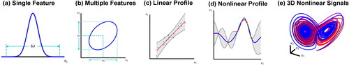
Once a network model is designed and developed, the next step is network monitoring. Statistical methods offer an opportunity to determine whether the network process is in control. Over the years, SPC has undergone a significant evolution. As shown in Figure 2, the inception of SPC concerned itself with single-feature, or univariate processes. However, there are various situations where multiple features are present. Monitoring each feature independently may be insufficient when considering the possibility of covariances. Thus, multivariate feature monitoring was developed (Montgomery, 2020). Nonetheless, some processes may be characterized by a profile or function. To this end, Kang and Albin (2000) establish a method to monitor linear profiles. Although linear profiles are common, there is the possibility that some profiles are nonlinear. One proposed technique by Zhou et al. (2006) for nonlinear profile monitoring integrates SPC with the Haar wavelet transform. Wavelet SPC allows for the detection of process shifts, as well as their location and magnitude within the evaluated signal. Zhang et al. (2018a) propose a multi-tier approach to the nonlinear profile monitoring endeavor. Signals are first preprocessed to align the profiles and remove noise. Sensors are then clustered based on their cross-correlation matrix. After clustering, multichannel principal component analysis is employed to extract sensor cluster features. Derived local monitoring statistics are then fused to create global monitoring statistics according to the top-$R$ rule. The aforementioned profile monitoring scheme was eventually adapted to handle weak correlations and sparse out-of-control patterns (Zhang et al., 2018b). This feat was achieved by incorporating lasso penalties into the determination of the monitoring statistics. Rather than using the top-$R$ rule, an exponential moving average-based likelihood ratio statistic was developed to handle SPC. Also, real-world sensor signals may contain a large degree of irregularity or have chaotic features. To solve this issue, Chen et al. (2019) deal with nonlinear signal dynamics through the creation of the pattern-frequency tree approach. Application of this pattern-frequency tree demonstrates promise in detecting anomalies within nonlinear dynamical systems.

Figure 2. SPC has evolved from univariate monitoring of a single feature to joint monitoring of multiple features. Monitoring of linear and then nonlinear profiles has been the natural development. However, there is a limitation in the ability to monitor nonlinear signals in three or more dimensions.

The progression of SPC methods has greatly propelled quality improvements in the realm of smart manufacturing. Traditional quality measurements can be metrics (e.g., geometric dimensionality) or profiles (linear or nonlinear). However, sensor signals are indirect observations of quality characteristics in the underlying process. When these signals are nonlinear, nonstationary, and have many dimensions, traditional SPC methods tend to be limited. Standard univariate or multivariate monitoring cannot handle the behavior of a process that can be represented as a profile or function. Likewise, profile monitoring is more applicable for calibration measures or sensor profiles that are cyclical in nature and display high degrees of repeatability. Nonlinear signals pose significant challenges to profile-based techniques. There is an urgent need to investigate flux dynamics for statistical monitoring of nonlinear dynamical processes. Flux dynamical analysis produced through VS network models have received little attention in the field of SPC. Further development of network flux monitoring is needed to fill existent gaps.

3. Research methodology

The flow diagram of a VS network model for sensor-based process monitoring is given in Figure 3. Physical sensors collect time-varying signals pertinent to operational dynamics of a complex system. These signals contain implicit dynamical information about the system that is conducive to process monitoring and control. Further, we proposed to deploy a network of VSs to extract and monitor flux dynamics in the signal space. These VSs conform to the signal’s trajectory and topology in many dimensions using self-organizing principles.

Figure 3. VS network model for sensor-based process monitoring. Physical sensors produce time-varying signals. Virtual sensors (shown in red) are placed within the signal space to produce a set of dynamic network profiles. These network profiles have their FR extracted and monitored for decision support.

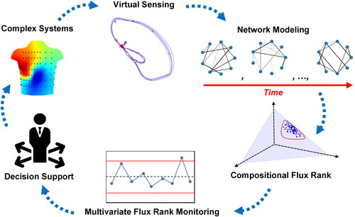
Then, we develop a network model to characterize and represent real-time flux-dynamics among these VSs, in which each node represents a VS, while edges are signal flux among sensors. A new FR algorithm is also designed to characterize and quantify influx and outflux transition dynamics around each sensor. However, the FR is compositional and cannot be adequately monitored with traditional multivariate control charts. Therefore, we propose an isometric log-ratio transform to design and develop new FR statistics and pertinent control charts to perform virtual sensing and monitoring of complex systems. Insights from the special FR control charts can be further used to drive decision support and process improvements.

3.1. Self-organizing virtual sensing

To drive the creation of a generalized VS networking framework, we propose to leverage self-organizing principles to optimize the placement of anchoring VSs within the multidimensional signal space. By the name “self-organizing,” we are referring to a competitive mechanism where VSs will compete with one another for the right to sense and partition the signal space according to its distribution and topological features. VSs are allocated for the purpose of space coverage as follows:

• Within the signal space: There will be $i=1,\dots ,I-1$ VSs deployed to form a collection of coverage regions on the multidimensional signal trajectory. Self-organization is, therefore, referring to the learning of geometric characteristics of signal trajectory for optimal placement of these $I-1$ VSs within the signal space.

• Outer signal space: Although nonlinear signals dynamically evolve in the space, it is not uncommon that system dynamics are confined to the signal trajectory with certain degrees of uncertainty. Thus, the outer signal space represents a counterpart of the signal space and describes the general outer space (i.e., out-of-control regions) in which the signal does not reside. Hence, an extra VS, i.e., the $I$^th VS, is necessary to represent the coverage of the outer signal space and sense the underlying out-of-control behaviors.

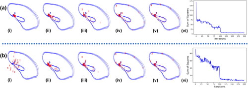
The process of self-organizing VSs within the signal space can be seen in Figure 4 and is given by Algorithm 1. As shown, the self-organizing methodology converges to the signal’s topological features regardless of the initial placement of the VSs. Topological convergence curves shown in the figure confirm the optimal placement of the VSs. Let ${\mathbf{x}}^{(t)}={\left(x_1^{(t)},\dots ,x_m^{(t)}\right)}^{\prime }$ be a signal vector, where $m$ is the dimensionality of the signal vector and $t=1,\dots ,T$ is the length of the multidimensional signal. The distance of ${\mathbf{x}}^{(t)}$ to a VS $r_i$ is given by $d_i=\Vert r_i-{\mathbf{x}}^{(t)}\Vert ,i=1,\dots ,I-1,$ where $i$ is the VS index and $r_i$ is the VS location in the signal space. The I^th VS, being located in the outer signal space, represents the outer signal space in general. The distance vector $\mathbf{d}=(d_1,\dots ,d_{I-1})\prime$ is fed into a competitive function where each VS excites itself and inhibits all others. This competitive function $\mathrm{\Phi }$ is given by, (1) $${\mathrm{\Phi }}_i=\{\begin{array}{c}1, i=i^{\mathrm{*}}\\ 0, i\ne i^{\mathrm{*}}\end{array}\text{ where }{d}_{i^{\mathrm{*}}}\le d_i,\forall i\text{ and }{i}^{\mathrm{*}}\le i,\forall d_i=d_{i^{\mathrm{*}}}$$(1)

Figure 4. Illustration of self-organizing VS featuring VCG signals given two initial VS configurations (a & b) after (i) 0, (ii) 50, (iii) 100, (iv) 150, and (v) 200 iterations, as well as the performance convergence curve (vi). Here, the performance metric is computed as the sum of squared distances from the signals to the nearest VS when the number of iterations increases.

The self-organizing procedure will reward the VS that wins the competition as well as its neighboring VSs using the Kohonen rule, (2) $$r_i^{(k+1)}=r_i^{\left(k\right)}+\psi \left({\mathbf{x}}^{\left(t\right)}-r_i^{\left(k\right)}\right),\mathrm{ }\forall i\in {\mathrm{\Lambda }}_{i^{\mathrm{*}}}\left(\tilde{d}\right)$$(2) where $k=1,\dots ,K$ is the training iteration, $\psi$ is the learning rate, and ${\mathrm{\Lambda }}_{i^{\mathrm{*}}}\left(\tilde{d}\right)$ is the neighborhood that captures the indices of neighboring VSs that lie within a radius $\tilde{d}$ of the winning VS $r_{i^{\mathrm{*}}},$ (3) $${\mathrm{\Lambda }}_{i^{\mathrm{*}}}\left(\tilde{d}\right)=\left\{i,\Vert r_i-r_{i^{\mathrm{*}}}\Vert \le \tilde{d}\right\}$$(3)

When ${\mathbf{x}}^{(t)}$ is presented to the network, the winning VS and its neighbors will all move towards ${\mathbf{x}}^{(t)}.$ Each time a new signal vector is presented, the closest VS will win the competition. The winning VS and its neighbors will move closer to the input signal and, by extension, to each other. The VSs have two existent behaviors: First, they will distribute themselves over the signal space in the learning process. Second, they will move towards the locations of neighboring VSs. These behaviors cause the VSs to self-organize so that they partition the signal space according to its distribution and topological features. This competitive process will continue until reaching the maximum number of iterations $K_r$ or until the VS locations converge.

Our proposed self-organization of the VS network within the signal space is different from minimum energy design (Joseph et al., 2015) in the field of Design Of Experiments (DOE) and spring-electrical model in the domain of variable clustering (Liu and Yang, 2018). In the DOE setting of minimum energy design, the spatial location of a design point will not change during the experiment. The algorithm will optimize the spatial location of the next design point given that spatial locations of previous design points are fixed. By contrast, variable clustering seeks to self-organize the dataspace of variables. Variables are represented as charged particle nodes that repel one another. To counteract this force, edges between the nodes are represented as springs that pull the nodes back together. The optimization objective in the case of variable clustering is to minimize the total energy of the network.

Algorithm 1:

Self-Organizing Virtual Sensor Placement

Input: Sensor Signals ${\mathbf{x}}^{(t)},t=1,\dots ,T,$

Radius $\tilde{d},$ Learning rate $\psi ,$

Maximum Iterations $K_r,$ Tolerance ${ϵ}_r$

Output: Optimal Virtual Sensor Locations $r_i,i=1,\dots ,I-1$

1: Set $k=0$

2: Initialize $r_i^{(0)},\forall i=1,\dots ,I-1$

3: do

4:  for $t=1,\dots ,T$ do

5:   Calculate $\mathbf{d}={\left(d_1,\dots ,d_{I-1}\right)}^{\prime }$

6:   Compute $\mathbf{\Phi }={\left({\mathrm{\Phi }}_1,\dots ,{\mathrm{\Phi }}_{I-1}\right)}^{\prime }$

7:   $i^{\mathrm{*}}=\mathrm{arg max}({\mathrm{\Phi }}_1,\dots ,{\mathrm{\Phi }}_{I-1})$

8:   Find ${\mathrm{\Lambda }}_{i^{\mathrm{*}}}\left(\tilde{d}\right)$

9:   $r_i^{\left(k+1\right)}=r_i^{(k)}+\psi \left(x^{\left(t\right)}-r_i^{(k)}\right),\mathrm{ }\forall i\in {\mathrm{\Lambda }}_{i^{\mathrm{*}}}\left(\tilde{d}\right)$

10:  end for

11:  $k=k+1$

12: while $\Vert r_i^{(k)}-r_i^{(k-1)}\Vert >{ϵ}_{r\mathrm{ }}\forall i=1,\dots ,I-1$ and $k<K_r$

13: return $r_i^{(k)},i=1,\dots ,I-1$

However, this investigation drives VSs iteratively to compete for the right to represent input signals. Winners of each competition and their neighboring VSs are rewarded by being drawn closer to these input signals. After a competition is held for all input signals, the process repeats until a maximum number of iterations are reached, or until convergence. The resulting layout of VSs after the self-organizing process captures the distribution and topological features of the signal space. The competitive mechanism makes VSs move and compete for the right to sense signals in this self-organizing design.

3.2. VS network modeling and FR

The self-organized VSs will be responsible for sensing the inflows and outflows within the signal space. Thus, a VS will become excited when its coverage region is entered by an incoming signal. Likewise, the VS will cease being excited as the signal departs its coverage region. To determine which VS is excited at a given time, we assign a categorical identifier to each VS. As nonlinear signals pass by the closest VS in the signal space, a time series of categorical values will be generated to record the path of transversed VSs. By tracking the order and duration of VS excitation, we can extract the dynamical information present within the input signal. Nonetheless, only considering the “closest” VS within the signal space is limited in its handling of the outer signal space and, by extension, of uncertainty. Signal vectors may be at a great distance away from all VSs in the signal space, but still technically “closer” to one VS over another. To account for the outer signal space, one may consider truncating the VS coverage regions such that they have strictly defined boundaries. Signals falling outside these strictly defined regions would be sensed by the $I$^th VS, which exists in the outer signal space. Unfortunately, there is no granularity in uncertainty to this truncation approach. The signal is either fully attributed to one of the $I-1$ VSs in the signal space or fully attributed to the $I$^th VS placed in the outer signal space. Thus, the “closest” VS at a given time would either be fully known or fully uncertain. This uncertainty disparity is especially problematic near coverage region boundaries, due to oversensitivity causing the outer signal space to become overrepresented in the observed signal dynamics. The overrepresentation of the outer signal space consequently produces many false positives during process monitoring. Therefore, there is an urgent need to account for the outer signal space (and by extension signal uncertainty) with finer granularity.

To mitigate the issues presented regarding the outer signal space, we introduce an affinity measure ${\gamma }^{(t)},$ where $0<{\gamma }^{(t)}\le 1.$ We assume that each VS region within the signal space has a Gaussian coverage, each with mean $r_i$ and bandwidth matrix $B_i.$ Assuming there are $I-1$ VSs in the signal space, suppose that each Gaussian has weight ${\varpi }_i=N_i/T,$ where $N_i$ is the number of signals closest to VS $r_i.$ The distribution of each signal would then follow, (4) $$\mathrm{Pr}\left\{{\mathbf{x}}^{\left(t\right)}\right\}=\sum _{i=1}^{I-1}{\varpi }_i\mathcal{N}\left({\mathbf{x}}^{\left(t\right)}\right|r_i,B_i)$$(4) where $\mathcal{N}(\cdot )$ describes a multivariate normal distribution. The affinity ${\gamma }_i$ can be calculated for all the VS coverage regions as, (5) $${\gamma }_i\left({\mathbf{x}}^{\left(t\right)}\right)=\frac{{\varpi }_i\mathcal{N}\left({\mathbf{x}}^{\left(t\right)}{r}_i,B_i\right)}{{\sum }_{i^{\prime }=1}^{I-1}{\varpi }_{i^{\prime }}\mathcal{N}\left({\mathbf{x}}^{\left(t\right)}{r}_{i^{\prime }},B_{i^{\prime }}\right)}\mathrm{ }i=1,2,\cdots ,I-1$$(5) where ${\sum }_{i=1}^{I-1}{\gamma }_i\left({\mathbf{x}}^{\left(t\right)}\right)=1.$ The $I$^th sensor in the outer signal space captures out-of-control behaviors (anomalies) present in the signals as they dynamically evolve over time and transverse the virtual sensors. Thus, anomalies are captured around each coverage region in the signal space, $\mathit{o}\left({\mathbf{x}}^{\left(t\right)}\right)={\mathbf{1}}_{\mathit{I}-1}-\mathit{\gamma }\left({\mathbf{x}}^{\left(t\right)}\right).$

Further, there is a pressing need to optimize the weight and bandwidth of each coverage region of VS $r_i.$ The sensitivity can be controlled by adjusting the bandwidth matrix $B_i,$ which alters the size and shape of the sensing region. The bandwidth matrix $B_i$ may be designed to form full, diagonal, or spherical coverage regions. Therefore, we propose a new procedure to estimate the optimal bandwidth matrix $B_i^{*},i=1,\dots ,I-1$ (and consequently the corresponding optimal weights ${\varpi }_i^{*}$), as shown in Algorithm 2.

Algorithm 2:

Estimation of Weight and Bandwidth Matrices

Input: VS Locations $r_i,i=1,\dots ,I-1,$ Sensor Signals ${\mathbf{x}}^{(t)},t=1,\dots ,T,$

Maximum Iterations $K_B,$ Tolerance ${ϵ}_B$

Output: Optimal Bandwidth Matrices and Gaussian Weights $B_i^{*},{\varpi }_i^{*}, i=1,\dots ,I-1$

1: Set $k=0$

2: Initialize $B_i^{(0)},{\varpi }_i^{(0)},\forall i=1,\dots ,I-1$

3: do

4:  Calculate ${\gamma }_i^{(k)}\left({\mathbf{x}}^{\left(t\right)}\right)=\frac{{\varpi }_i^{\left(k\right)}\mathcal{N}\left({\mathbf{x}}^{\left(t\right)}|r_i,B_i^{\left(k\right)}\right)}{{\sum }_{i^{\prime }=1}^{I-1}{\varpi }_{i^{\prime } }^{\left(k\right)}\mathcal{N}\left({\mathbf{x}}^{\left(t\right)}|r_{i^{\prime }},B_{i^{\prime } }^{\left(k\right)}\right)},$

$$\forall i=1,\dots ,I-1,t=1,\dots ,T$$

5:  $k=k+1$

6:  for $i=1,\dots ,I-1$ do

7:   ${\mathrm{\Gamma }}_i^{(k)}={\sum }_{t=1}^T{\gamma }_i^{(k-1)}\left({\mathbf{x}}^{\left(t\right)}\right)$

8:   $B_i^{(k)}=\frac{1}{{\mathrm{\Gamma }}_i^{(k)}}{\sum }_{t=1}^T{\gamma }_i^{(k-1)}\left({\mathbf{x}}^{\left(t\right)}\right)\left({\mathbf{x}}^{\left(t\right)}-r_i\right){\left({\mathbf{x}}^{\left(t\right)}-r_i\right)}^{\prime }$

9:   ${\varpi }_i^{(k)}=\frac{{\mathrm{\Gamma }}_i^{(k)}}{T}$

10:  end for

11: while $\Vert {\mathcal{L}}^{(k)}-{\mathcal{L}}^{(k-1)}\Vert >{ϵ}_B$ and $k<K_B$

12: return $B_i^{(k)},{\varpi }_i^{(k)},i=1,\dots ,I-1$

The inputs to the proposed Algorithm 2 are the VS locations $r_i,\forall i=1,\dots ,I-1,$ the signal ${\mathbf{x}}^{(t)},t=1,\dots ,T,$ convergence tolerance $ϵ,$ and the maximum iteration $K.$ First the iteration counter $k$ is set to zero. Next, the values $B_i^{(0)}$ and ${\varpi }_i^{(0)},\forall i=1,\dots ,I-1$ are initialized based on the present signals. Next, the method enters an iterative process of learning. In each iteration, the affinity ${\gamma }_i\left({\mathbf{x}}^{\left(t\right)}\right),\forall i=1,\dots ,I-1,t=1,\dots ,T$ is determined. Then, the iteration counter $k$ is incremented. Afterwards, for each VS $r_i,$ we calculate the total signal affinity ${\mathrm{\Gamma }}_i^{\left(k\right)}={\sum }_{t=1}^T{\gamma }_i^{(k-1)}\left({\mathbf{x}}^{\left(t\right)}\right)$ that are used to update both $B_i^{(k)}$ and ${\varpi }_i^{(k)},\forall i=1,\dots ,I-1.$ This process continues until the maximum number of iterations $K_B$ is reached or if the log likelihood of all signals $\mathcal{L}$ converges to tolerance ${ϵ}_B,$ where, (6) $$\mathcal{L}=\mathcal{ }\sum _{t=1}^T\log \hspace{0.17em}\left(\mathrm{Pr}\left\{{\mathbf{x}}^{\left(t\right)}\right\}\right)$$(6)

As a result, Algorithm 2 provides the estimate of optimal $B_i^{*}$ and ${\varpi }_i^{*},\forall i=1,\dots ,I-1$ for each coverage region.

Given bandwidths $B_i,i=1,\dots ,I-1$ and VS affinity functions ${\gamma }_i\left(\cdot \right),i=1,\dots ,I-1,$ we can formulate a representation of the signal’s state as ${\mathbf{x}}^{\left(t\right)}$ dynamically evolves over time $t.$ Let us denote the state of the system at time $t$ as $s^{(t)}=\underset{i}{\mathrm{argmax}}\left({\gamma }_i\left({\mathbf{x}}^{\left(t\right)}\right)\right),s^{(t)}\in \{1,\dots ,I-1\}.$ Likewise, let the affinity of the signal be ${\gamma }^{(t)}=\underset{i}{\max }\left({\gamma }_i\left({\mathbf{x}}^{\left(t\right)}\right)\right)$ while in state $s^{(t)}.$ The corresponding anomalies while in state $s^{(t)}$ are calculated as ${\mathit{o}}^{(t)}=1-{\gamma }^{(t)}.$ Therefore, we obtain the triplet ${[s,\gamma ,\mathit{o}]}^{(t)}$ for each signal vector when system dynamics pass through the network of VSs in the multidimensional space.

Algorithms 1 and 2 are performed utilizing a large quantity of in-control signals for the initialization of the VS network. Once the VS network is established, it can be leveraged for monitoring. Now, the question becomes: “How to construct the VS network and derive the probability transition matrix $P$ accounting for uncertainty?” The probability transition matrix $P$ should capture the stochastic behaviors of VS inflows and outflows when the signal is evolving over time. Therefore, we propose Algorithm 3 to generate the probability transition matrix $P,$ which takes the state and uncertainty pair ${[s,\gamma ,o]}^{(t)},t=1,\dots ,T$ as its input. The transitions will be among the $I$ VS regions in both the signal trajectory and the outer signal space, leading to a $I\times I$ matrix $P.$ For example, a state transition from a current state $s^{(t)}=i$ can go to either the next state $s^{(t+1)}=i\prime$ in the signal space or the state $I$ in the outer signal space. Therefore, the transition $P_{i{i}^{\prime }}$ is computed as $f\left({\gamma }^{\left(t\right)},{\gamma }^{\left(t+1\right)}\right),$ where $f(\cdot )$ is an interpolating function that accounts for the affinity levels in both states. Here, we use an average function $f\left(\cdot \right)=\left({\gamma }^{\left(t\right)}+{\gamma }^{\left(t+1\right)}\right)/2.$

Algorithm 3:

Probability Transition Matrix Generation

Input: ${[s,\gamma ,\mathit{o}]}^{(t)},t=1,\dots ,T$

Output: Probability Transition Matrix $P$

1: $P={\mathbf{0}}_{I,I},$ where $I$ is the total number of states

2: for $t=1,2, \dots ,T-1$ do

3:  $i=s^{(t)}, i^{\prime }=s^{(t+1)}$

4:  $P_{i{i}^{\prime }}=P_{i{i}^{\prime }}+f\left({\gamma }^{\left(t\right)},{\gamma }^{\left(t+1\right)}\right)$

5:  $P_{iI}=P_{iI}+f\left({\mathit{o}}^{\left(t\right)},{\mathit{o}}^{\left(t+1\right)}\right)$

6: end for

7: for $i=1,\dots ,I$ do

8:  if ${\sum }_{i^{\prime }=1}^I{P}_{i{i}^{\prime }}=0$ then

9:   $P_{i{i}^{\prime }}=\frac{1}{I}, \forall i^{\prime }=1,\dots ,I$

10:  else

11:   $P_{i{i}^{\prime }}=\frac{P_{i{i}^{\prime }}}{{\sum }_{i^{″}=1}^I{P}_{i{i}^{″}}},\forall i^{\prime }=1,\dots ,I$

12:  end if

13: end for

14: return $P$

As shown in Algorithm 3, we start by initializing $P$ to ${\mathbf{0}}_{I,I},$ which is a $I\times I$ matrix of zeros. For the entire signal from $t=0$ to $T-1,$ the transition $P_{i{i}^{\prime }}$ will be increased by $f\left({\gamma }^{\left(t\right)},{\gamma }^{\left(t+1\right)}\right),$ while $P_{iI}$ will be increased by $f\left({\mathit{o}}^{\left(t\right)},{\mathit{o}}^{\left(t+1\right)}\right).$ Next, we regularize each row of the transition matrix $P_{i\cdot },i=1,\dots ,I$ and convert its entries into a probability. Should the sum of a row $P_{i\cdot }$ be equal to zero, each entry of the row is set to $1/I.$ Otherwise, each entry in the row is divided by the row sum ${\sum }_{i^{\prime }=1}^I{P}_{i{i}^{\prime }}.$ The new Algorithm 3 provides a way to transform VS flux dynamics into a probability transition matrix while accounting for signal noises and system uncertainty. Analyzing the inflows and outflows associated with each VS provides a new sensor-based approach to monitor a spatiotemporal process. In this regard, each VS acts a quality inspection station that studies the passage of signals into and out of the VS network.

The relative flux between VSs is consolidated into a single rank measure, known as the FR. Algorithm 4 transforms a probability transition matrix $P$ into a corresponding FR $\mathit{\varrho }$ that is compositional in nature. Determining the FR first entails performing an adjustment on $P$ to obtain an irreducible matrix $\tilde{P}.$ Certain subgraph structures present in $P$ result in $\mathit{\varrho }$ having zero entries. Should $\mathit{\varrho }$ have any zero entries, it will fail to capture the flux dynamics surrounding the corresponding VSs. Thus, for a $I\times I$ transition matrix $P,$ this adjustment is performed by computing $\tilde{P}=\left(1-q\right)P+\frac{q}{I}{\mathbf{1}}_{I, I}.$ Note that ${\mathbf{1}}_{I,I}$ is an $I\times I$ matrix of ones, the parameter $q$ is an adjustment factor, where $0\le q<1.$ Typically, $q$ is set to be closer to zero so that transition dynamics are not overly obfuscated by the matrix adjustment. Let ${\mathit{\varrho }}^{(0)}=\frac{1}{I}{\mathbf{1}}_I$ be an initial FR value, where ${\mathbf{1}}_I$ is a $I$-length vector of all ones. The flux rank ${\mathit{\varrho }}^{(k+1)}$ is updated by left multiplying $\tilde{P}$ with ${\mathit{\varrho }}^{(k)}$ in each iteration. The process continues until convergence or reaching a maximum number of iterations $K_{\varrho }.$

Algorithm 4:

Flux Rank

Input: Probability Transition Matrix $P,$ Adjustment Factor $q,$

Tolerance ${ϵ}_{\varrho },$ Maximum Iterations $K_{\varrho }$

Output: Flux rank $\mathit{\varrho }$

1: Let $\tilde{P}=\left(1-q\right)P+\frac{q}{I}{\mathbf{1}}_{I,I}$

2: Let ${\mathit{\varrho }}^{(0)}=\frac{1}{I}{\mathbf{1}}_I$ and $k=0$

3: do

4:  ${\mathit{\varrho }}^{(k+1)}=\tilde{P}{\mathit{\varrho }}^{(k)}$

5:  $k=k+1$

6: while $\Vert {\mathit{\varrho }}^{(k)}-{\mathit{\varrho }}^{(k-1)}\Vert >{ϵ}_{\varrho }$ and $k<K_{\varrho }$

7: return ${\mathit{\varrho }}^{(k)}$

Granularity in the outer signal space is captured through the VS affinity measure associated with a signal’s current state. Taking this affinity-based granularity into account when generating the VS network’s probability transition matrix is reflected in VS inflows and outflows. Therefore, the FR generated under this affinity framework gives a more accurate representation of the relative flux between all VSs.

3.3. FR statistical monitoring

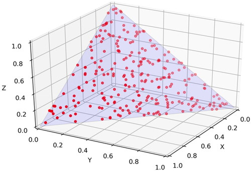
Note that FR features are always compositional in nature. A vector is considered compositional if its elements sum to one. For example, the vector $\tilde{\mathbf{x}}={\left(0.25, 0.60,0.15\right)}^{\prime }$ is compositional. Compositional data are embedded within the simplex space. A simplex represents a generalization of the triangle to an arbitrary number of dimensions. Thus, FR features are constrained to the $I$-dimensional simplex ${\mathcal{S}}^I.$ Due to this constraint, the FR features cannot be evaluated under standard SPC frameworks. Figure 5 shows an example of compositional data constrained to the ${\mathcal{S}}^3$ simplex in the ${\mathbb{R}}^3$ space, but they are also embedded into a two-dimensional plane that takes a triangular shape.

Figure 5. Illustration of compositional data constrained to ${\mathcal{S}}^3.$ The simplex is shown in a blue plane, whereas datapoints are depicted in red.

Multinomial data represents a certain variety of compositional data. The Pearson ${\chi }^2$ statistic is used to monitor multinomial data (and in some cases, Dirichlet data, which is also compositional). However, this statistic is not generally applicable to all forms of compositional data, due to issues involving the upper control limit. Oftentimes with non-multinomial data, the upper control limit is too small. Boyles et al. (1997) encounter a similar issue when designing SPC principles to non-multinomial data. An adjustment of the Degrees Of Freedom (DOF) was proposed to remedy this issue. Therefore, we develop a FR version of this general compositional ${\chi }^2$ statistic to monitor the FR with the adjusted DOF, $${\mathrm{\Pi }}^2=\sum _{i=1}^I\frac{{\left({\varrho }_i-{\overline{\varrho }}_i\right)}^2}{{\overline{\varrho }}_i}$$ (7) $$\frac{\nu {\mathrm{\Pi }}^2}{E\left({\mathrm{\Pi }}^2\right)}\sim {\chi }_{\nu ;\varrho }^2$$(7) where $E(\cdot )$ is the expected value function, and $\nu$ are the effective DOF. The effective DOF can be found by calculating, (8) $$\nu =⌈\frac{2{\left[E\left({\mathrm{\Pi }}^2\right)\right]}^2}{\mathit{Var}\left({\mathrm{\Pi }}^2\right)}⌉$$(8) where $⌈\cdot ⌉$ is the ceiling function, and $\mathit{Var}(\cdot )$ is the variance function. Hence, the upper control limit of the FR ${\chi }^2$ statistic can be obtained as ${\chi }_{\alpha ,\nu ;\varrho }^2.$

Multivariate monitoring schemes typically involve the Hotelling $T^2$ statistic in its design. Vives-Mestres et al. (2014) shows that the Hotelling $T^2$ statistic is inadequate to handle compositional data. Compositional data comes with a major pain point: multicollinearity is always encountered due to the restrictions imposed by the simplex. Furthermore, simply removing one of the variables involved in the multicollinearity or restructuring the covariance matrix with spectral analysis does not address the peculiarities specific to compositions; either approach produces a hyper-ellipsoid confidence region that may easily exceed the bounds of the simplex. These techniques also fail to address the unique types of in-control patterns that may occur within the simplex space.

Hence, we propose to leverage the isometric log-ratio (ilr) transform (Egozcue et al., 2003) to tackle this dilemma. Transforming our FR composition $\mathit{\varrho }$ with ilr yields coordinates $\mathit{\zeta }.$ $$\mathit{\varrho }\stackrel{\mathit{ilr}}{\to }\mathit{\zeta }={\left({\zeta }_1,\dots ,{\zeta }_{I-1}\right)}^{\prime }$$ (9) $$\mathit{\zeta }=U^T\cdot \log \hspace{0.17em}\mathit{\varrho }$$(9) Note that $U=({\mathbf{u}}_1,\dots ,{\mathbf{u}}_{I-1})$ is a $I\times (I-1)$ matrix that represents an orthonormal basis with respect to any $I$-dimensional composition. The FR feature $\mathit{\varrho }$ can be recovered from $\mathit{\zeta }$ with the inverse ilr transform, $$\mathit{\zeta }\stackrel{il{r}^{-1}}{\to }{\mathit{\varrho }=\left({\varrho }_1,\dots ,{\varrho }_I\right)}^{\prime }$$ (10) $$\mathit{\varrho }=\mathcal{C}(\exp \hspace{0.17em}\left(U\mathit{\zeta }\right))$$(10) The function $\mathcal{C}\left(\cdot \right)$ is the closure of the input vector, which functions according to Definition 1.

Definition 1.

Let $\mathcal{C}(\cdot )$ be the closure operation, (11) $$\mathcal{C}\left(\mathit{\zeta }\right)={\left(\frac{{\zeta }_1}{\sum _{i=1}^{I-1}{\zeta }_i},\mathrm{ }\dots ,\frac{{\zeta }_{I-1}}{\sum _{i=1}^{I-1}{\zeta }_i}\right)}^{\prime }$$(11)

The principle of working on coordinates accommodates the translation of standard statistics into any sample space with a structure of Euclidean vector space; to do so, we must be working on a coordinate representation that is held with respect to an orthonormal basis. Therefore, transformation of $\mathit{\varrho }$ into coordinates $\mathit{\zeta }$ with the orthonormal basis $U$ will preserve its statistical properties.

Definition 2.

Let ${\mathbf{u}}_i\in {\mathbb{R}}^d,i=1,2,\dots ,I-1$ be orthonormal with respect to the ordinary Euclidean inner product in ${\mathbb{R}}^I$ and constitute a basis of a $(I-1)$-dimensional linear subspace, $${\mathbf{u}}_i=\sqrt{\frac{i}{i+1}}\cdot {\left(\frac{1}{i},\dots ,\frac{1}{i},-1,0,\dots ,0\right)}^{\prime }$$ where the $-1$ element occurs as the $(i+1)$^th position of the vector. See the proof of the structure of $U$ and statistical properties of ilr transform of FR features in the Appendix.

Suppose there are $J$ segments of in-control sensor signals, we can obtain FR features ${\mathit{\varrho }}^{(j)}$ for the j^th segment, where $j=1,\dots ,J.$ After ilr transform from $\mathit{\varrho }$ to $\mathit{\zeta },$ we estimate isometric FR coordinate mean $\overline{\mathit{\zeta }}$ and covariance matrix $S_{\zeta }.$ We then derive the FR Hotelling $T^2$ statistic, (12) $${\left(T_{\zeta }^2\right)}^{\left(j\right)}={\left({\mathit{\zeta }}^{\left(j\right)}-\overline{\mathit{\zeta }}\right)}^{\prime }{S}_{\zeta }^{-1}\left({\mathit{\zeta }}^{\left(j\right)}-\overline{\mathit{\zeta }}\right)$$(12) The upper control limit of the $T_{\zeta }^2$ chart is computed as, (13) $$UC{L}_{T_{\zeta }^2}=\frac{(I-1)(J+1)(J-1)}{J^2-J(I-1)}{F}_{\left(\alpha ,I-1,J-I+1\right)\mathrm{ }}$$(13) The value of $F_{\left(\alpha ,I-1,J-I+1\right) }$ is the upper $1-\alpha$ percentile of the $F$ distribution with $J$ segments of sensor signals with isometric FR coordinates of dimensionality $I-1.$

In addition, we propose to design and develop the General Likelihood Ratio (GLR) test in order to handle compositional data. Kan and Yang (2017) used GLR statistics to monitor the image profiles from a biomanufacturing process, however, this is not applicable to compositional data. As discussed, dealing with compositions comes with a whole host of unique challenges. Here, we leverage the ilr transform to develop new GLR statistics for monitoring the FR features generated from virtual sensing of nonlinear signals.

Suppose that $\mathit{\zeta }$ follows a multivariate normal distribution with mean ${\mathit{\mu }}_{0;\zeta }$ and covariance ${\mathrm{\Sigma }}_{\zeta }.$ Should a process shift occur at the $\tau$^th network profile, the mean will shift to ${\mathit{\mu }}_{1;\zeta }.$ We therefore have the following hypothesis test, (14) $$\{\begin{array}{c}{H}_0:E{\left[{\mathit{\zeta }}^{\left(j\right)}\right]}_{j=1}^{\tau }=E{\left[{\mathit{\zeta }}^{\left(j\right)}\right]}_{j=\tau +1}^J={\mathit{\mu }}_{0;\zeta }\\ H_1:E{\left[{\mathit{\zeta }}^{\left(j\right)}\right]}_{j=1}^{\tau }\ne E{\left[{\mathit{\zeta }}^{\left(j\right)}\right]}_{j=\tau +1}^J={\mathit{\mu }}_{1;\zeta }\end{array}$$(14) We can then derive the following likelihood function for the in-control data, (15) $$L\left({\mathit{\mu }}_{0;\zeta }\right)=\prod _{j=1}^J\frac{1}{{\left(2\pi \right)}^{(I-1)/2}{\left|{\mathrm{\Sigma }}_{\zeta }\right|}^{1/2}}\exp \hspace{0.17em}\left(-\frac{1}{2}{\left({\mathit{\zeta }}^{\left(j\right)}-{\mathit{\mu }}_{0;\zeta }\right)}^{\prime }{\mathrm{\Sigma }}_{\zeta }^{-1}\left({\mathit{\zeta }}^{\left(j\right)}-{\mathit{\mu }}_{0;\zeta }\right)\right)$$(15) Should the process shift at $\tau ,$ the likelihood function becomes, (16) $$L\left({\mathit{\mu }}_{0;\zeta },{\mathit{\mu }}_{1;\zeta }\right)={\left(\frac{1}{{\left(2\pi \right)}^{(I-1)/2}{\left|{\mathrm{\Sigma }}_{\zeta }\right|}^{1/2}}\right)}^J\times \prod _{j=1}^{\tau }\exp \left(-\frac{1}{2}{\left({\mathit{\zeta }}^{\left(j\right)}-{\mathit{\mu }}_{0;\zeta }\right)}^{\prime }{\mathrm{\Sigma }}_{\zeta }^{-1}\left({\mathit{\zeta }}^{\left(j\right)}-{\mathit{\mu }}_{0;\zeta }\right)\right)\times \prod _{j=\tau +1\mathrm{ }}^J\exp \left(-\frac{1}{2}{\left({\mathit{\zeta }}^{\left(j\right)}-{\mathit{\mu }}_{1;\zeta }\right)}^{\prime }{\mathrm{\Sigma }}_{\zeta }^{-1}\left({\mathit{\zeta }}^{\left(j\right)}-{\mathit{\mu }}_{1;\zeta }\right)\right)$$(16) The mean shift after $\tau$ can be estimated with, (17) $${\widehat{\mathit{\mu }}}_{J,\tau ;\zeta }=\frac{1}{J-\tau }\sum _{j=\tau +1\mathrm{ }}^J{\mathit{\zeta }}^{\left(j\right)}$$(17) The maximum log likelihood ratio statistic can be derived as follows, (18) $$\begin{array}{c}{R}_{J;\zeta }=\log \hspace{0.17em}\frac{L({\mathit{\mu }}_{0;\zeta },{\mathit{\mu }}_{1;\zeta })}{L\left({\mathit{\mu }}_{0;\zeta }\right)}\\ R_{J;\zeta }=\log \hspace{0.17em}\frac{\underset{0\le \tau <J}{\max }L({\mathit{\mu }}_{0;\zeta },{\widehat{\mathit{\mu }}}_{J,\tau ;\zeta })}{L\left({\mathit{\mu }}_{0;\zeta }\right)}\end{array}$$(18) The FR GLR statistic can be calculated with, (19) $$R_{J;\zeta }=\underset{0\le \tau <J}{\max }\frac{J-\tau }{2}{\left({\widehat{\mathit{\mu }}}_{J,\tau ;\zeta }-{\mathit{\mu }}_{0;\zeta }\right)}^{\prime }{\mathrm{\Sigma }}_{\zeta }^{-1}\left({\widehat{\mathit{\mu }}}_{J,\tau ;\zeta }-{\mathit{\mu }}_{0;\zeta }\right)$$(19) We can now replace ${\mathit{\mu }}_{0;\zeta }$ and ${\mathrm{\Sigma }}_{\zeta }$ with $\overline{\mathit{\zeta }}\mathrm{ }$ and $S_{\zeta },$ giving us, (20) $$R_{J;\zeta }=\underset{0\le \tau <J}{\max }\frac{J-\tau }{2}{\left({\widehat{\mathit{\mu }}}_{J,\tau ;\zeta }-\overline{\mathit{\zeta }} \right)}^{\prime }{S}_{\zeta }^{-1}\left({\widehat{\mathit{\mu }}}_{J,\tau ;\zeta }-\overline{\mathit{\zeta }} \right)$$(20) To reduce the computational complexity, online monitoring can be considered with sliding windows when $J$ is large. A sliding window $\omega$ is used to prune some historical data during the computation. The upper control limit is established with the estimated distribution of the FR GLR statistic from in-control data. (21) $$R_{J;\zeta }=\underset{J-\omega \le \tau <J}{\max }\frac{J-\tau }{2}{\left({\widehat{\mathit{\mu }}}_{J,\tau ;\zeta }-\overline{\mathit{\zeta }}\mathrm{ }\right)}^{\prime }{S}_{\zeta }^{-1}\left({\widehat{\mathit{\mu }}}_{J,\tau ;\zeta }-\overline{\mathit{\zeta }}\mathrm{ }\right)$$(21)

4. Experimental design and materials

The proposed methodology is evaluated and validated with nonlinear Lorenz systems and physiological signal case studies. In all experimental cases, we utilize a statistical significance level of $\alpha =0.01,$ FR adjustment factor $q=0.001,$ FR convergence criteria ${ϵ}_{\varrho }={10}^{-4},$ and maximum number of FR iterations $K_{\varrho }=1000.$ All bandwidth parameters are designed to be spherical upon initialization. Experimental design and materials are detailed for each scenario as in the following sections.

4.1. Nonlinear Lorenz signals

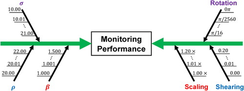
The Lorenz attractor is a well-known chaotic system whose signal vector is represented by ${\left(x,y,z\right)}^{\prime }.$ The system changes according to $\dot{x}=\sigma (y-x),$ $\dot{y}=x\left(\rho -z\right)-y,$ $\dot{z}=xy-\beta z,$ where $\sigma ,\rho ,$ and $\beta$ are model parameters. We assume that the system is in control for the set of parameters $\sigma =10,\rho =20,\beta =1.$ Shifts in these model parameters will cause the system to become out of control. We vary parameters according to Figure 6 to test the performance of the proposed VS monitoring framework.

Figure 6. Lorenz (left) and VCG (right) study cause and effect diagram.

Each Lorenz process is represented by a signal generated according to its input parameters. Each scenario generates 1000 independent realizations of the process. To evaluate the monitoring performance of each statistical method, we compute detection power, which is the proportion of out-of-control processes correctly detected. Additionally, we determine the average run length (ARL₁) before out-of-control behavior is detected by each technique.

4.2. VCG signals

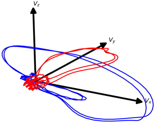
The human heart generates nonlinear and nonstationary physiological signals. When this electrical activity is monitored along orthogonal planes of the body, a three-dimensional signal known as the VCG is obtained. Yang et al. (2013) showed that spatiotemporal aberrations in the VCG are pertinent to the presence of disease occurring in different sectors of the heart. As shown in Figure 7, different segments of the VCG experience affine distortions in the presence of diseases, such as like Myocardial Infarctions (MI). These distortions take the form of affine rotation, scaling, and shearing.

Figure 7. VCG for a healthy control (blue) and myocardial infarction (red).

The experiments performed in the VCG signal study are conducted by employing affine transformations for out-of-control signal generation, also see the cause-and-effect diagram in Figure 6. It is assumed that various degrees of rotation, scaling, and shearing occur when the heart is moving away from the in-control state. The degree of these perturbations can be seen in Figure 6. We join multiple affine transformations together to generate the out-of-control signals with the combinational effects of scaling, rotation and shearing, according to,

Table

Scaling: $M_c=\left[\begin{array}{ccc}{c}_x& 0& 0\\ 0& c_y& 0\\ 0& 0& c_z\end{array}\right]$	X-Axis Rotation: $M_{{\theta }_x}=\left[\begin{array}{ccc}1& 0& 0\\ 0& \cos \hspace{0.17em}{\theta }_x& -\sin \hspace{0.17em}{\theta }_x\\ 0& \sin \hspace{0.17em}{\theta }_x& \cos \hspace{0.17em}{\theta }_x\end{array}\right]$	Y-Axis Rotation: $M_{{\theta }_y}=\left[\begin{array}{ccc}\cos \hspace{0.17em}{\theta }_y& 0& \sin \hspace{0.17em}{\theta }_y\\ 0& 1& 0\\ -\sin \hspace{0.17em}{\theta }_y& 0& \cos \hspace{0.17em}{\theta }_y\end{array}\right]$
Z-Axis Rotation: $M_{{\theta }_z}=\left[\begin{array}{ccc}\cos \hspace{0.17em}{\theta }_z& -\sin \hspace{0.17em}{\theta }_z& 0\\ \sin \hspace{0.17em}{\theta }_z& \cos \hspace{0.17em}{\theta }_z& 0\\ 0& 0& 1\end{array}\right]$		Shearing: $M_h=\left[\begin{array}{ccc}1& h_{xy}& h_{xz}\\ h_{yx}& 1& h_{yz}\\ h_{zx}& h_{zy}& 1\end{array}\right]$

Note that $\theta$ describes an angle of rotation (in radians) about a particular axis, $c$ describes scaling with respect to a particular axis, and $h$ refers to various forms of shearing. For the purposes of this investigation, process shifts are held with respect to a transformation’s mean. Rotation and scaling case studies are shifted with respect to the $z$-axis, thus only ${\theta }_z$ and $c_z$ are perturbed. Shearing is only perturbed with respect to $h_{zy}.$

Each VCG realization is represented by a time series of heartbeats, which are generated according to the pertinent affine shifts. Each case evaluated generates 1000 heartbeats. Detection power is, once again, employed to evaluate the performance of the statistical methods previously discussed. Likewise, we also determine the ARL₁ performance for the VCG study.

5. Experimental results

5.1. Flux Rank

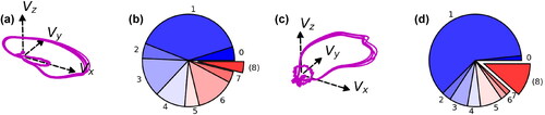
The multidimensional nonlinear signals may be transformed into a corresponding FR when exposed to a network of VSs. An intermediate step in the FR calculation is the production of a timeseries of state and affinity pairs. Recall that the state timeseries represent the dynamic path traversed VSs taken by the signal trajectory. Each state record in the timeseries has its own associated affinity value, which is also evolving with time. A case study of this FR computation, showing the intermediate step, is shown in Figure 8. Since the FR is compositional, it is represented as a pie chart. The FR element associated with the outer signal space is represented in exploded view.

Figure 8. (a) VCG signal for a single beat. Corresponding (b) state time series and (c) affinity time series as well as (d) a pie chart showing the associated FR composition.

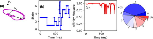
The FR can reveal out-of-control behavior in a signal. As a result, there is an observable shift in both the VCG signal and its corresponding FR when a patient suffers from a MI. Such a shift is from healthy to MI is shown in Figure 9 where the shift in the VCG signal is visually noticeable. As expected, the FR exhibits a similarly noticeable shift. The FR element corresponding to the outer signal space has a much larger value for the MI signal than for the healthy signal. In particular, the healthy FR outer signal space value is 3.90% of the FR composition whereas the MI outer signal space value is 11.52% of the FR composition.

Figure 9. (a) Healthy VCG signals with the corresponding (b) healthy signal FR compared against (c) MI VCG signals with the corresponding (d) MI signal FR.

5.2. Statistical monitoring of nonlinear dynamic systems – Lorenz

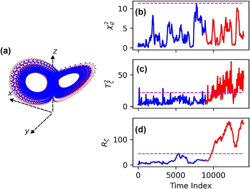
An online monitoring case study of the Lorenz study was performed with 10,000 in-control signal points being generated with parameters $\sigma =10,\rho =20,\beta =1.$ The subsequent 5000 out-of-control signal points were generated with parameters $\sigma =10,\rho =20,\beta =1.1.$ As shown in Figure 10, it is very difficult to visually detect the process shift. Thus, a sliding window of size 1000 with a step size of 50 is utilized to generate relevant monitoring statistics. Eight VSs are deployed and self-organized in the signal space alongside a ninth VS placed in the outer signal space. Control charts for these statistics are depicted in Figure 10. The purple dashed line on each chart represents the control limit. It may be noted that the FR ${\chi }^2$ chart is unable to detect the process shift. The FR Hotelling $T^2$ and GLR charts are both able to detect the shift with equal amounts of competence. A window size of $\omega =10$ is used for the creation of the FR GLR chart.

Figure 10. (a) Lorenz system signal parameters shifting from $\sigma =10,\rho =20,\beta =1$ (blue dots) to $\sigma =10,\rho =20,\beta =1.1$ (red lines), and the time evolution of (b) ${\chi }_{\varrho }^2,$ (c) $T_{\zeta }^2$ and (d) $R_{\zeta }.$

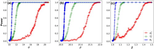
Figure 11 shows the performance comparison among the evaluated statistical methods for all Lorenz model configurations based on the experimental design in Figure 6. For each scenario, 1000 in-control samples and 1000 out-of-control samples were generated. Each sample had 500 points in its signal. The results show that the FR GLR chart is able to correctly detect all out-of-control networks once $\sigma$ reaches 11, as $\rho$ reaches 20.25, and as $\beta$ reaches 1.05. Likewise, the FR Hotelling $T^2$ chart demonstrates full detection power as $\sigma$ reaches 13, as $\rho$ reaches 20.75, and as $\beta$ reaches 1.15. The FR ${\chi }^2$ chart achieves 100% detection power as $\sigma$ reaches 20, as $\rho$ reaches 21.75, and as $\beta$ reaches 1.4. Thus, the FR GLR method demonstrates superior detection capabilities for all parameter shifts in comparison to the FR $T^2$ and ${\chi }^2$ methods. FR GLR can detect very minute changes to the control parameters. Additionally, for all parameter shifts, the FR $T^2$ procedure shows better detection capability than the FR ${\chi }^2$ technique.

Figure 11. Performance comparison of the detection power of FR ${\chi }^2, T^2,$ and GLR methods with varying parameters (a) $\sigma ,$ (b) $\rho ,$ and (c) $\beta$ .

5.3. Statistical monitoring of multidimensional physiological signals – VCG

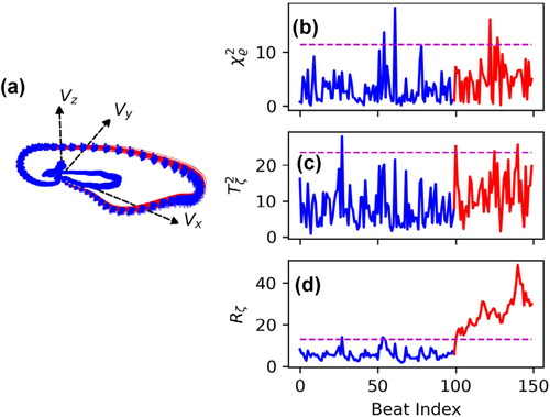
An online case study of the VCG study was performed with 100 generated in-control beats. Cardiac activity is not deterministic. Therefore, there is assumed to be some level of baseline distortion in the signal, in the form of rotation, shearing and scaling. We apply in-control affine distortions with normally distributed parameters, according to, (22) $$\begin{array}{c}{\theta }_{\ell }\sim \mathcal{N}\left(0,{\left[\frac{\pi }{256}\right]}^2\mathrm{ }\right),\mathcal{ }\ell \in \{x,y,z\}\\ c_{\ell }\sim \mathcal{N}\left({1,\mathrm{ }\left[0.01\right]}^2\right),\ell \in \{x,y,z\}\\ h_{\ell {\ell }^{\prime }}\sim \mathcal{N}\left({0,\mathrm{ }\left[0.01\right]}^2\right),\ell ,{\ell }^{\prime }\in \left\{x,y,z\right\}\end{array}$$(22)

After the 100 in-control beats are generated, the subsequent 50 out-of-control beats were generated with a mean shift in $h_{zy}$ of 0.03, giving $h_{zy}\sim \mathcal{N}({0, \left[0.01\right]}^2).$ This shift represents a miniscule change to the expected amount of affine shearing in the signal. The difference between the in-control and out-of-control signals is difficult to detect visually in Figure 12. Eight VSs were deployed and self-organized in the signal space alongside a ninth VS placed in the outer signal space. When assessing the control charts shown in Figure 12, one will notice that neither the FR ${\chi }^2$ chart nor the FR Hotelling $T^2$ chart is capable of detecting the process shift. By contrast, the FR GLR chart can detect the process shift. A window size of $\omega =10$ is utilized for the creation of the FR GLR chart.

Figure 12. (a) Healthy VCG signal (blue dots) experiencing a mean shift in shearing parameter $h_{zy}$ of 0.03 (red lines), and the time evolution of (b) ${\chi }_{\varrho }^2,$ (c) $T_{\zeta }^2$ and (d) $R_{\zeta }.$

Figure 13 portrays the comparison between three benchmark statistical methods for all VCG model configurations based on the design in Figure 6. For each scenario, 1000 in-control beats and 1000 out-of-control beats were generated. The results show that the FR GLR chart is able to correctly detect all out-of-control networks once ${\theta }_z$ reaches 0.050, as $c_z$ reaches 1.25, and as $h_{zy}$ reaches 0.050. Likewise, the FR Hotelling $T^2$ chart demonstrates full detection power as ${\theta }_z$ reaches 1.125, as $c_z$ reaches 1.075, and as $h_{zy}$ reaches 0.100. The FR ${\chi }^2$ chart achieves 100% detection power as ${\theta }_z$ reaches 0.150, as $c_z$ reaches 1.15, and as $h_{zy}$ reaches 0.175. Once again, like with the Lorenz study, the FR GLR procedure demonstrated the best detection power when compared with the other methods. The next most sensitive method was the FR $T^2$ procedure. The FR ${\chi }^2$ chart performed the worst across the board.

Figure 13. Performance comparison of the detection power of FR ${\chi }^2,\mathrm{ }{T}^2,$ and GLR methods with varying parameters (a) ${\theta }_z,$ (b) $c_z,$ and (c) $h_{zy}.$

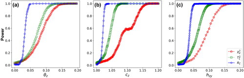
We evaluated and benchmarked three control charts on their strengths and limitations for monitoring system dynamics. In both Lorenz and VCG cases, it is shown that the FR GLR statistic outperforms both FR Hotelling $T^2$ and FR ${\chi }^2$ statistics. The FR GLR can detect the process shift for both the online Lorenz and VCG studies. The FR Hotelling $T^2$ can detect the process shift for the online Lorenz study, but is unable to detect the shift present in the online VCG study. The FR ${\chi }^2$ chart was unable to detect the process shift in both online Lorenz and VCG cases. In addition, power analysis demonstrates the sensitivity of each FR chart. Across the board, for both Lorenz and VCG studies, it is shown that the FR GLR chart has higher sensitivity to parametric distortions than the FR Hotelling $T^2$ and FR ${\chi }^2$ charts. Experimental results show that the FR GLR chart achieves better performance for VS-based process monitoring than the FR Hotelling $T^2$ chart and the FR ${\chi }^2$ chart.

6. Conclusions

Sensor technologies generate time-varying signals, which encapsulate the dynamics of a complex system. Effective monitoring of these dynamics is imperative to fostering decision support and, therefore, maintaining system control. Nonetheless, these signals are often nonstationary and nonlinear, thus posing a challenge for traditional quality monitoring praxis. As a result, there is an urgent need to design and develop new sensor-based monitoring techniques. In this investigation, we propose a new VS network for sensor-based process monitoring. Self-organization allows a network of VSs to be placed within the signal space according to topological features. The VS network then captures flux dynamics by sensing both the signal’s state and its VS affinity. These flux dynamics are consolidated into a single FR measure. Signal distortions ultimately have implication on the FR vector, meaning that monitoring FR can reveal out-of-control behavior. To this end, ilr statistical techniques are leveraged to handle the compositional nature of the FR. New control charts, such as the new FR GLR, Hotelling $T^2$ and ${\chi }^2$ charts, are designed to monitor the FR.

These new FR monitoring methods display varying degrees of sensitivity. According to Lorenz and VCG online case studies, the FR GLR chart outperforms the other two FR charts. Power analyses corroborate these findings. Thus, the FR GLR chart is the preferred method when compared to the FR ${\chi }^2$ and $T^2$ charts. Ultimately, the VS network model and FR statistics provide a new sensor-based monitoring framework for scrutinizing multidimensional signals that are nonlinear and nonstationary. Nonlinear and chaotic dynamics have posed significant challenges on statistical process control and data analytics. The proposed VS Network (VSN) methodology is promised to be generally applicable for sensor-based monitoring of nonlinear dynamical systems.

Finally, the proposed VSN can be alternatively formulated as nonlinear signal fitting or feature extraction problems. However, it should be noted that this article is not focused on placing virtual sensors for signal reconstruction. In contrast, this article focuses more on the utilization of virtual sensors to monitor the evolving influx and outflux dynamics of nonlinear signals, also called flux dynamical analysis. In future, nonlinear signal fitting with the network placement of VSs should be investigated. As such, this new idea can be further studied to treat VSN as the model and the nonlinear signal as the process. In addition, nonlinear feature extraction is an umbrella term for a large plurality of methods that extract features from nonlinear data, but the VSN approach is aimed at the placement of virtual sensors for flux dynamical analysis. In future work, another new idea is to investigate nonlinear manifold learning for the flux dynamical analysis, and then investigate the general applicability for sensor-based monitoring of nonlinear dynamical systems.

Additional information

Funding

The authors of this work would like to acknowledge the NSF grant MCB-1856132 and CMMI-1617148 for funding this research. Any opinions, findings, or conclusions found in this paper are those of the authors and do not necessarily reflect the views of the sponsors.

Notes on contributors

Alexander Krall

Alexander Krall is a PhD student in the Complex System Monitoring, Modeling and Analysis laboratory at the Harold and Inge Marcus Department of Industrial and Manufacturing Engineering, Pennsylvania State University. He received both his Bachelor of Science (2016) and Master of Science (2018) degrees in Industrial & Systems Engineering at the Rochester Institute of Technology. Alexander’s primary research areas are distributed security, differential privacy, and quality-driven data analytics pertinent to complex manufacturing and healthcare systems.

Daniel Finke

Dr. Daniel Finke is an Associate Research Professor in the Materials and Manufacturing Office at the Applied Research Laboratory, The Pennsylvania State University and the director of the Center for e-Design. Much of Dr. Finke’s experience in applied research and development is within the US Navy shipbuilding domain collaborating on projects in Advanced Manufacturing Enterprise with a focus on production and capacity planning, Industrial Internet of Things (IIoT), and manufacturing system modeling and analysis. Dr. Finke received his PhD in Industrial Engineering (2010) and MS in Industrial Engineering and Operations Research (2002) from the Pennsylvania State University and a BS in Industrial Engineering from New Mexico State University (2000). His current research interests include simulation-based decision support, planning and scheduling, heuristic algorithm development and implementation, agent-based simulation and modeling, and process improvement.

Hui Yang

Dr. Hui Yang is a Professor in the Harold and Inge Marcus Department of Industrial and Manufacturing Engineering at The Pennsylvania State University, University Park, PA. His research interests are sensor-based modeling and analysis of complex systems for process monitoring, process control, system diagnostics, condition prognostics, quality improvement, and performance optimization. He received the NSF CAREER award in 2015, and multiple best paper awards from the international IEEE, IISE and INFORMS conferences. Dr. Yang is the president (2017–2018) of IISE Data Analytics and Information Systems Society, the president (2015–2016) of INFORMS Quality, Statistics and Reliability (QSR) society, and the program chair of 2016 Industrial and Systems Engineering Research Conference (ISERC). He is also the department editor for IISE Transactions Healthcare Systems Engineering, as well as associate editors for IISE Transactions, IEEE Journal of Biomedical and Health Informatics (JBHI), IEEE Transactions on Automation Science and Engineering.

References

- Boyles, R.A. (1997) Using the chi-square statistic to monitor compositional process data. Journal of Applied Statistics, 24(5), 589–602.
- Chen, C.-B., Yang, H. and Kumara, S. (2019) A novel pattern-frequency tree for multisensor signal fusion and transition analysis of nonlinear dynamics. IEEE Sensors Letters, 3, 1–4.
- Chen, Y. and Yang, H. (2016) Heterogeneous recurrence representation and quantification of dynamic transitions in continuous nonlinear processes. The European Physical Journal B, 89(6), 155.
- Cheng, C., Kan, C. and Yang, H. (2016) Heterogeneous recurrence analysis of heartbeat dynamics for the identification of sleep apnea events. Computers in Biology and Medicine, 75, 10–18.
- Cheng, F.-T., Huang, H.-C. and Kao, C.-A. (2012) Developing an automatic virtual metrology system. IEEE Transactions on Automation Science and Engineering, 9(1), 181–188.
- Egozcue, J.J., Pawlowsky-Glahn, V., Mateu-Figueras, G. and Barceló-Vidal, C. (2003) Isometric logratio transformations for compositional data analysis. Mathematical Geology, 35(3), 279–300.
- Fortuna, L., Graziani, S., Rizzo, A. and Xibilia, M.G. (2007) Soft Sensors for Monitoring and Control of Industrial Processes, Springer, London.
- Funatsu, K. (2018) Process control and soft sensors, in Applied Chemoinformatics, John Wiley & Sons, Ltd., Weinheim, Germany, pp. 571–584.
- Hsieh, Y.-M., Lin, C.-Y., Yang, Y.-R., Hung, M.-H. and Cheng, F.-T. (2019) Automatic virtual metrology for carbon fiber manufacturing. IEEE Robotics and Automation Letters, 4(3), 2730–2737.
- Joseph, V.R., Dasgupta, T., Tuo, R. and Wu, C.F.J. (2015) Sequential exploration of complex surfaces using minimum energy designs. Technometrics, 57(1), 64–74.
- Kan, C. and Yang, H. (2017) Dynamic network monitoring and control of in situ image profiles from ultraprecision machining and biomanufacturing processes. Quality and Reliability Engineering International, 33(8), 2003–2022.
- Kang, L. and Albin, S.L. (2000) On-line monitoring when the process yields a linear profile. Journal of Quality Technology, 32(4), 418–426.
- Kim, Y. and Patel, J. (2010) Performance comparison of the R*-tree and the quadtree for kNN and distance join queries. IEEE Transactions on Knowledge and Data Engineering, 22(7), 1014–1027.
- Lin, B., Recke, B., Knudsen, J.K.H. and Jørgensen, S.B. (2007) A systematic approach for soft sensor development. ESCAPE-15, 31(5), 419–425.
- Liu, G. and Yang, H. (2018) Self-organizing network for variable clustering. Annals of Operations Research, 263(1), 119–140.
- Masuda, Y., Kaneko, H. and Funatsu, K. (2014) Multivariate statistical process control method including soft sensors for both early and accurate fault detection. Industrial & Engineering Chemistry Research, 53(20), 8553–8564.
- Montgomery, D.C. (2020) Introduction to Statistical Quality Control, 8th ed. Wiley, Hoboken, New Jersey.
- Papadimitriou, P., Dasdan, A. and Garcia-Molina, H. (2010) Web graph similarity for anomaly detection. Journal of Internet Services and Applications, 1(1), 19–30.
- Sadreazami, H., Mohammadi, A., Asif, A. and Plataniotis, K.N. (2018) Distributed-graph-based statistical approach for intrusion detection in cyber-physical systems. IEEE Transactions on Signal and Information Processing over Networks, 4(1), 137–147.
- Vives-Mestres, M., Daunis-I-Estadella, J. and Martín-Fernández, J.-A. (2014) Individual T2 control chart for compositional data. Journal of Quality Technology, 46(2), 127–139.
- Yang, H., Bukkapatnam, S.T. and Komanduri, R. (2012) Spatiotemporal representation of cardiac vectorcardiogram (VCG) signals. BioMedical Engineering OnLine, 11(1), 16.
- Yang, H., Kan, C., Liu, G. and Chen, Y. (2013) Spatiotemporal differentiation of myocardial infarctions. IEEE Transactions on Automation Science and Engineering, 10(4), 938–947.
- Yang, H., Liu, R. and Kumara, S. (2020) Self-organizing network modelling of 3D objects. CIRP Annals, 69(1), 409–412.
- Yang, W.-T., Blue, J., Roussy, A., Pinaton, J. and Reis, M.S. (2020) A structure data-driven framework for virtual metrology modeling. IEEE Transactions on Automation Science and Engineering, 17(3), 1297–1306.
- Zhang, C., Yan, H., Lee, S. and Shi, J. (2018a) Multiple profiles sensor-based monitoring and anomaly detection. Journal of Quality Technology, 50(4), 344–362.
- Zhang, C., Yan, H., Lee, S. and Shi, J. (2018b) Weakly correlated profile monitoring based on sparse multi-channel functional principal component analysis. IISE Transactions, 50(10), 878–891.
- Zhang, Y., Yang, C., Huang, K., Zhou, C. and Li, Y. (2021) Robust structure identification of industrial cyber-physical system from sparse data: A network science perspective. IEEE Transactions on Automation Science and Engineering, 1–15.
- Zhou, S., Sun, B. and Shi, J. (2006) An SPC monitoring system for cycle-based waveform signals using Haar transform. IEEE Transactions on Automation Science and Engineering, 3(1), 60–72.
- Zou, N. and Li, J. (2017) Modeling and change detection of dynamic network data by a network state space model. IISE Transactions, 49(1), 45–57.