Dynamic pricing of regulated field services using reinforcement learning

Abstract

Resource flexibility and dynamic pricing are effective strategies in mitigating uncertainties in production systems; however, they have yet to be explored in relation to the improvement of field operations services. We investigate the value of dynamic pricing and flexible allocation of resources in the field service operations of a regulated monopoly providing two services: installations (paid-for) and maintenance (free). We study the conditions under which the company can improve service quality and the profitability of field services by introducing dynamic pricing for installations and the joint management of the resources allocated to paid-for (with a relatively stationary demand) and free (with seasonal demand) services when there is an interaction between quality constraints (lead time) and the flexibility of resources (overtime workers at extra cost). We formalize this problem as a contextual multi-armed bandit problem to make pricing decisions for the installation services. A bandit algorithm can find the near-optimal policy for joint management of the two services independently of the shape of the unobservable demand function. The results show that (i) dynamic pricing and resource management increase profitability; (ii) regulation of the service window is needed to maintain quality; (iii) under certain conditions, dynamic pricing of installation services can decrease the maintenance lead time; (iv) underestimation of demand is more detrimental to profit contribution than overestimation.

Keywords:

• Dynamic pricing
• quality management
• regulation
• reinforcement learning

1. Introduction

The successful application of incentive (dynamic) pricing in various industries (e.g., hotels and retail) continues to encourage innovative ideas for companies to improve their operations. We consider the case of installation and maintenance services, where the customer pays to receive an installation service (e.g., a telephone line or broadband) currently at a fixed price and then pays an ongoing service charge with the expectation that if a fault occurs with the equipment, it will be repaired without having to incur additional costs. The current practice is to deploy a fixed number of employees during periods of sustained levels of demand (e.g., Monday to Friday, 9 a.m. to 5 p.m.) and then to use more flexible solutions to meet unexpected levels of demand, such as overtime or on-call employees.

The maintenance service has a stochastic demand with seasonal and weekly fluctuations, whereas the demand for installations is stable throughout the week. The demands for these two services are independent of each other. Figure 1 summarizes the total demand per day. The average number of installations, maintenance, and total jobs completed per day decreases during the week, being the highest on Monday and the lowest on Friday.

Figure 1. Average number of installation and maintenance jobs completed per day.

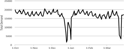
The company’s database used in this article includes daily historical data on maintenance and installation intake, the total workforce size, a description of the engineer’s skill types, planned and unplanned absences, the number of jobs completed, the number of overtime workers, and the work stack left. In the database, planned absences range from about 18% to 30% (Christmas time), with a mean of 23.5%, whereas unplanned absences range from 0% to 6.3%, with a mean of 2.5%. It is clear that even in the short-term unplanned absences are a significant cost for the company.

We aim to mitigate the mismatch of demand and supply by jointly managing the maintenance and installation services. We propose that the employees for both services be combined and a dynamic pricing policy be used for the installation service. A higher price can be charged for installations during high maintenance demand, and price discounts are offered on installations during periods of low demand for maintenance. The pricing scheme aims to work as a tool to reduce the number of overtime technicians, increasing efficiency in managing field service operations. This improvement, nonetheless, needs to strictly respect the quality targets, primarily measured by the service lead times. Their specific characteristics are central to our contribution. The assumptions required to approximate the problem of the motivating case are as follows. The maintenance service is free and subject to a service level agreement, the demand for the two services is not correlated, and additional resources are available at a higher cost; the maintenance service has to be provided within a specific time frame following the request because of regulations, and the firm has a fixed number of available workers for each day of the week.

This article models the problem as a contextual multi-armed bandit problem and uses a reinforcement learning technique to approximate optimal prices. The main managerial results are as follows. Dynamic pricing combined with resource management increase profitability. The regulation of the service window is needed to maintain the service quality. Dynamic pricing of installation services can decrease the maintenance lead time. The underestimation of demand is more detrimental to profitability than demand overestimation. The main contribution of this article is to consider the interplay of shared resources and dynamic pricing of one service to meet the regulation constraint of the other free service.

The rest of this article is organized as follows: Section 2 provides a literature review; Section 3 models the interaction between dynamic pricing and resource management; Section 4 uses reinforcement learning to determine an optimal pricing policy; Section 5 summarizes the major analytical results; Section 6 summarizes the numerical results. Finally, Section 7 concludes the article.

2. Related literature

Resource flexibility and dynamic pricing (also known as responsive pricing) are two effective strategies for mitigating uncertainties in production systems (Hariharan et al., 2020). In production systems, resource flexibility requires the firm to invest in a flexible resource capable of producing multiple products to adjust supply to the realized demand. Responsive pricing influences demand to reduce the mismatch between demand and supply, reducing demand volatility and investment in production capacity. For production systems, resource flexibility comes with a higher investment cost in possibly more expensive facilities. It is more valuable when product demands are negatively correlated, and substitutability among products is low. As product substitutability increases, it becomes cost-effective to switch demand through responsive pricing (Lus and Muriel, 2009).

Extensive reviews on the interplay of pricing and resource management have been provided by Chan et al. (2004), Chod and Rudi (2005), Ding et al. (2007), Chen and Simchi-Levi (2012). More recently, Luong et al. (2017) provides an extensive review of pricing theory for resource management about the 5G wireless network; Sharghivand et al. (2021) survey auction mechanism design for cloud resource management and pricing. Bish and Suwandechochai (2010) considered two substitutable products with one flexible capacity. They studied how the degree of product substitution and the level of operational postponement affect optimal capacity decisions. Goyal and Netessine (2010) investigated the trade-off between volume and product flexibility about the impact of demand correlations for a two-product setting. They found that volume flexibility helps mitigate aggregate demand uncertainty and product flexibility helps with individual demand uncertainty for each product. Ceryan et al. (2013) studied a joint mechanism for dynamic pricing and resource flexibility to manage demand and supply mismatches across multiple products. They found that the presence of flexible resources helps to maintain stable price differences across different items and significantly improves profits. An overview of multi-product models is given in Chen and Chen (2015).

More recently, Chen and Chen (2018) explored dynamic pricing for two substitute products with several business rules, considering both inter-product and inter-temporal demand substitution; Hariharan et al. (2020) investigate capacity uncertainties and disruptions caused by temporary production shutdowns, faulty manufacturing processes, and natural or man-made disasters; Vicil (2021) studied inventory rationing as a strategy to help organizations to limit the growth in inventory through inventory pooling and differentiating services among different customer classes. Asheralieva and Niyato (2020) provide a detailed survey of resource management and pricing in the internet of things with blockchain as a service, using reinforcement and deep learning.

Our company does not have complete information about the installation service’s demand process in our study. For this reason, learning (i.e., the bandit algorithm) is proposed to estimate the installation service’s value function and near-optimal pricing decisions. The algorithm aims to determine the “right prices” to maximize profit. Nonetheless, if from the learning process it arises that a fixed fee is the most profitable strategy, then the optimal policy keeps the price constant.

As the decision-maker does not know the probabilities associated with the different states of demand for installations services, and as the firm has incomplete knowledge of how the pricing policy impacts customer behavior, it seems that the multi-armed bandit problem is an excellent tool to study this problem as, although simple, it can capture the complexities of economic systems (Sutton and Barto, 1998). The contextual multi-armed bandits are ideal for capturing non-stationary environments (i.e., the underlying model of the changes in the problem settings over time) where some of the variables characterizing the process are observable. Still, other variables are such that the decision-maker may be unaware of their existence. Misra et al. (2019) modeled the problem with incomplete information using multi-armed bandits with statistical machine learning to identify consumer demand functions.

The multi-armed bandit problem is not amenable to an analytical solution. Instead, it is studied by numerical methods, which account for the necessary learning and required optimization used by the decision-maker to maximize profit and revenue or increase efficiency. For this reason, we build on existing literature by using reinforcement learning. The ease of adopting learning models across industries has increased with greater accessibility to data and increased storage capacity. Reinforcement learning is shown to be a powerful tool for dynamic pricing (Cheng, 2009; den Boer, 2015; Rana and Oliveira, 2015).

Kim et al. (2016) effectively uses reinforcement learning algorithms to price electricity and learn customers’ behavior dynamically. Maestre et al. (2019) consider a reinforcement learning pricing model which includes fairness in the measured reward to allocate goods equally between different groups of customers. Bondoux et al. (2020) study the use of reinforcement learning for airline revenue management, showing that exploration costs should be considered in the algorithm. Kastius and Schlosser (2021) use reinforcement learning to solve dynamic pricing problems in competitive settings.

This article is the first to consider applying reinforcement learning to find near-optimal pricing strategies, implicitly considering demand and capacity uncertainties for field service operations.

3. Modeling the field service operations

This is a two-stage model (Table A.1, in the Appendix, summarizes the notation.). In the first stage, we make installation pricing decisions using information about expected demand (maintenance and installation) and expected absent workers. In the second stage, once the actual demand is realized, as a recourse action, the number of overtime workers required to satisfy demand is calculated, taking into consideration the lead time constraints and actual absent workers.

The firm’s planning horizon is a week. The decisions are made for every working day t $\in$ $\{1,2,..,T\},$ where T is the number of working days. We assume a fixed number of contracted engineers, which is in line with the company’s current practice. On any given day, the maximum number of workers assigned to installation and maintenance services is f_t; this already considers planned absences. At stage 1, the decision variables are the number of technicians, at day t, who are assigned to maintenance services ($e_t^M$), and the price charged for installation at time t, p_t. These prices are calculated taking into account the expected demand and the available capacity, $f_t-e_t^M,$ and the respective number of technicians assigned to installations, $e_t^I.$ Then, at stage 2, after observing demand for both types of services, for a given day t, we need to compute the number of technicians working overtime in installations ($o_t^I$) and maintenance ($o_t^M$). The daily overtime salary of a technician is λ₀.

There is a set of stochastic variables that condition the field service operations problem at day t: first, the number of absent workers for installation ($a_t^I$) and maintenance ($a_t^M$) services; second, the new demand for installation ($d_t^I$) and maintenance ($d_t^M$) services,

Additionally, these are the auxiliary variables used in the model. For each day t: (i) the work stacks for installation ($S_t^I$) and maintenance ($S_t^M$) services are cumulative variables representing the number of jobs in the respective queues, and are indicated by capital letters; (ii) the lead time of maintenance jobs $L_t^M$ and the maximum number of days, $\overline{L},$ imposed by the regulator as part of the quality of service; (iii) the productivity per technician assigned to installation (β^I) and maintenance (β^M). The engineer’s productivity is determined by the number of jobs the engineer can complete in a day.

The model is summarized by programs (1) and (2). We aim to find a pricing policy that maximizes the expected revenue and minimizes the expected cost of overtime work. For this reason, in the program (1), we constrain the solution to meet expected demand and quality constraints.

According to the problem design, we estimate demand for expected maintenance jobs, calculate the resources required to meet the lead time constraint, and, hence, determine the available resources for installation jobs. Then, the capacity available for installation on different days is used to derive a pricing policy. The prices are displayed before the actual demand is realized and are such that the allocated resources are sufficient to meet demand. The major uncertainty factor is not the level of demand on a given day, as bookings are made in advance, and paying customers are unlikely to drop the appointments. The most crucial uncertainty source is the number of technicians available for maintenance and installation and, therefore, the need for overtime work. For this reason, in the recourse problem (2), we use the number of overtime hours required from the available technicians as, in general, we do not expect technicians to be reallocated to a different type of task.

The decisions in the program (1) are made once a week, given the expected demand for maintenance and installation and the expected number of absent workers, where the number of engineers, $e_t^M,$ and $e_t^I$ are non-negative integers, and the prices p_t are positive real numbers. The central feature of this optimization procedure is the inclusion of decisions made at different times: the initial allocation of technicians and the pricing of installation services are decided in the first stage when demand and the number of absent workers are both unknown. The expectation used as a basis for these stochastic variables requires knowledge of the probabilities associated with different demand levels and the number of absentees for all possible installation prices. (1a) $$\underset{p_t,e_t^M,e_t^I}{\max }\hspace{1em}\sum _{t=1}^T\mathbb{E}\left(d_t^I\right)p_t-\sum _{t=1}^T\mathbb{E}\left(o_t^I+o_t^M\right){\lambda }_0$$(1a) (1b) $$\begin{array}{c}s\mathit{ubject}to:\\ \mathbb{E}\left(d_t^M\right)\le {\beta }^M\left(e_t^M-\mathbb{E}\left(a_t^M\right)\right),\hspace{1em}\hspace{1em}\hspace{1em}\forall t\end{array}$$(1b) (1c) $$\mathbb{E}\left(d_t^I\right)={\beta }^I\left(e_t^I-\mathbb{E}\left(a_t^I\right)\right),\hspace{1em}\hspace{1em}\forall t$$(1c) (1d) $$\mathbb{E}\left(d_t^I\right)=D(p_1,\dots ,p_T),\hspace{1em}\forall t$$(1d) (1e) $$\mathbb{E}\left(S_t^M\right)\le \overline{L}{\beta }^M\left(e_t^M-\mathbb{E}\left(a_t^M\right)\right),\hspace{1em}\forall t$$(1e) (1f) $$e_t^M+e_t^I\le f_t,\hspace{1em}\hspace{1em}\hspace{1em}\hspace{1em}\hspace{1em}\forall t$$(1f) (1g) $$e_t^{\mathit{j}}\ge 0,\hspace{1em}\hspace{1em}\hspace{1em}\hspace{1em}j=I,M,\hspace{1em}\hspace{1em}\forall t$$(1g) (1h) $$p_t\ge 0,\hspace{1em}\hspace{1em}\hspace{1em}\hspace{1em}\hspace{1em}\hspace{1em}\forall t$$(1h)

The firm’s objective is to maximize the expected weekly revenue from installations, as represented by (1a)(1a) $$\underset{p_t,e_t^M,e_t^I}{\max }\hspace{1em}\sum _{t=1}^T\mathbb{E}\left(d_t^I\right)p_t-\sum _{t=1}^T\mathbb{E}\left(o_t^I+o_t^M\right){\lambda }_0$$(1a) . It combines the capacities for maintenance and installations with dynamic pricing; the demand for installation services is influenced by the maintenance demand to manage resources better and reduce the need for technicians’ overtime. The price charged for an installation at day t, p_t, is a function, possibly nonlinear, of the expected demand for installation and maintenance services each day and the available resources. Therefore, this is a bi-level optimization problem with incomplete information.

Equations (1b)(1b) $$\begin{array}{c}s\mathit{ubject}to:\\ \mathbb{E}\left(d_t^M\right)\le {\beta }^M\left(e_t^M-\mathbb{E}\left(a_t^M\right)\right),\hspace{1em}\hspace{1em}\hspace{1em}\forall t\end{array}$$(1b) to (1e)(1e) $$\mathbb{E}\left(S_t^M\right)\le \overline{L}{\beta }^M\left(e_t^M-\mathbb{E}\left(a_t^M\right)\right),\hspace{1em}\forall t$$(1e) relate the decisions on the number of technicians allocated to the different tasks to the expected demand and number of absences on any given day. These are unusual constraints as they require knowledge of the probabilities associated with the unobserved demand and behavior of employees and are estimated by the firm. In the first stage, for each day, the decision-maker chooses the number of technicians assigned to the two jobs without knowing the actual demand and the number of absent workers. These decisions are based on the probability associated with the different scenarios. In the second stage, after observing demand and the number of absent workers for each day t, the number of workers required to meet demand is calculated.

For the maintenance service, (1b)(1b) $$\begin{array}{c}s\mathit{ubject}to:\\ \mathbb{E}\left(d_t^M\right)\le {\beta }^M\left(e_t^M-\mathbb{E}\left(a_t^M\right)\right),\hspace{1em}\hspace{1em}\hspace{1em}\forall t\end{array}$$(1b) is the equilibrium condition, which specifies that we allocate enough resources to maintenance services to meet expected demand. In contrast, at the same time, constraint (1e)(1e) $$\mathbb{E}\left(S_t^M\right)\le \overline{L}{\beta }^M\left(e_t^M-\mathbb{E}\left(a_t^M\right)\right),\hspace{1em}\forall t$$(1e) specifies that the expected waiting time for the service is within the limits of quality. This constraint imposes that the expected stack size of maintenance jobs is within the quality constraints. The constraint considers the expected extent of technicians available for the job. However, it does not take into consideration the expected extent of overtime work as this resource should be used exceptionally. In the first stage, we do not plan overtime work; we prefer to use our contracted technicians to manage demand.

On average, overtime is equal to the number of hours of absent work. Still, as we prefer to use the cheaper resource, we need to subtract expected absences, so these are compensated by regular technicians instead of overtime work. Overtime work is still used to cover for unexpected absences. This is a complex set of constraints as we have a cumulative variable $S_t^M$ interacting with the decision variables $e_t^M.$ Nonetheless, the relationship between these variables is linear, as discussed in Proposition 5.2. On the other hand, the management of installations is more straightforward than maintenance service management. As the firm can use price to avoid peak demand and control the number of services it needs to provide, the lead time is unimportant. Instead, it attempts to meet the expected number of requests for new installations each day, and there is no need to control the size of the work stack.

Similarly, constraint (1c)(1c) $$\mathbb{E}\left(d_t^I\right)={\beta }^I\left(e_t^I-\mathbb{E}\left(a_t^I\right)\right),\hspace{1em}\hspace{1em}\forall t$$(1c) specifies that given the expected number of workers free to provide installation services, and the respective expectation about absenteeism, the price set needs to be such that the expected demand equals the resources expected to be available for this service. Constraint (1d)(1d) $$\mathbb{E}\left(d_t^I\right)=D(p_1,\dots ,p_T),\hspace{1em}\forall t$$(1d) is the demand function, which states that at any given time, the demand for installations is a function (possibly nonlinear) of the prices for each day of the week. Therefore, a customer decides when to have the installation service provided by comparing the prices across all the days of the same week. Constraint (1f)(1f) $$e_t^M+e_t^I\le f_t,\hspace{1em}\hspace{1em}\hspace{1em}\hspace{1em}\hspace{1em}\forall t$$(1f) represents the upper bound on the number of technicians available to be allocated to both services. Likewise, constraints (1g)(1g) $$e_t^{\mathit{j}}\ge 0,\hspace{1em}\hspace{1em}\hspace{1em}\hspace{1em}j=I,M,\hspace{1em}\hspace{1em}\forall t$$(1g) and (1h)(1h) $$p_t\ge 0,\hspace{1em}\hspace{1em}\hspace{1em}\hspace{1em}\hspace{1em}\hspace{1em}\forall t$$(1h) state that both the number of technicians and the installation price are non-negative.

The expected number of workers allocated to overtime work needs to be learned over time. After observing demand and absenteeism then, the actual overtime work is minimized in the program (2), which is a deterministic cost minimization problem with decisions (assumed to be non-negative real numbers) taken every day of the working week. This means that first, at the start of the week, we maximize the expected revenue. Then, in the second stage, each day, we minimize costs. (2a) $$\begin{array}{c}\text{For}\mathrm{ }\text{all}t:\\ \underset{o_t^I,o_t^M}{\min }\hspace{1em}(o_t^I+o_t^M){\lambda }_0\end{array}$$(2a) (2b) $$\begin{array}{c}s\mathit{ubject}to:\\ d_t^I\le {\beta }^I\left(e_t^I-a_t^I+o_t^I\right),\hspace{1em}\end{array}$$(2b) (2c) $$d_t^I=F(p_1,\dots ,p_T)\hspace{1em}$$(2c) (2d) $$S_t^M\le \overline{L}{\beta }^M\left(e_t^M-a_t^M+o_t^M\right),\hspace{1em}$$(2d) (2e) $$S_t^{\mathit{j}}=S_{t-1}^{\mathit{j}}+d_t^{\mathit{j}}-{\beta }^{\mathit{j}}\left(e_t^{\mathit{j}}-a_t^{\mathit{j}}+o_t^{\mathit{j}}\right),\hspace{1em}\text{If}\hspace{1em}t\in \{2,..,T\},\hspace{1em}j=I,M,$$(2e) (2f) $$S_t^{\mathit{j}}=S_0^{\mathit{j}}+d_t^{\mathit{j}}-{\beta }^{\mathit{j}}\left(e_t^{\mathit{j}}-a_t^{\mathit{j}}+o_t^{\mathit{j}}\right),\hspace{1em}\text{If}t=1\hspace{1em}j=I,M,$$(2f) (2g) $$o_t^{\mathit{j}}\ge 0,\hspace{1em}j=I,M.$$(2g) In the linear program (2), at the second stage, after observing demand and the number of absent workers, the firm minimizes the cost of overtime work (2a)(2a) $$\begin{array}{c}\text{For}\mathrm{ }\text{all}t:\\ \underset{o_t^I,o_t^M}{\min }\hspace{1em}(o_t^I+o_t^M){\lambda }_0\end{array}$$(2a) subject to the constraints regarding the obligation to meet the demand for installation (2b)(2b) $$\begin{array}{c}s\mathit{ubject}to:\\ d_t^I\le {\beta }^I\left(e_t^I-a_t^I+o_t^I\right),\hspace{1em}\end{array}$$(2b) and keep the minimum level of service quality (2d)(2d) $$S_t^M\le \overline{L}{\beta }^M\left(e_t^M-a_t^M+o_t^M\right),\hspace{1em}$$(2d) . This second stage problem is solved daily after demand is known and the number of absent workers is observed.

Inequalities (2b)(2b) $$\begin{array}{c}s\mathit{ubject}to:\\ d_t^I\le {\beta }^I\left(e_t^I-a_t^I+o_t^I\right),\hspace{1em}\end{array}$$(2b) and (2g)(2g) $$o_t^{\mathit{j}}\ge 0,\hspace{1em}j=I,M.$$(2g) describe how the number of overtime technicians assigned to installations is computed. When the actual demand exceeds expectations, the number of overtime technicians assigned to the task is increased to meet the actual demand. (This recourse measure is required because the prices are posted before the actual demand is observed.) When demand is less than expected, the overtime work is set to zero, as enough technicians are assigned to meet the demand requirements. $D(p_1,\dots ,p_T)$ is the expected demand function and $F(p_1,\dots ,p_T)$ is the realized or actual demand function: these demand functions are unobservable, complex to define. The price elasticity of demand is assumed to be non-zero, so the monopolist is limited in the ability to raise prices. This limitation arises both from consumer behavior and the potential for regulatory intervention.

In the second stage, after observing demand and absent workers, the firm determines the required number of overtime technicians. This decision depends on the observed demand and lead time constraint (2d)(2d) $$S_t^M\le \overline{L}{\beta }^M\left(e_t^M-a_t^M+o_t^M\right),\hspace{1em}$$(2d) .

As ${\mathrm{\beta \hspace{0.17em}}}^{\mathit{j}}(e_t^{\mathit{j}}-a_t^{\mathit{j}}+o_t^{\mathit{j}})$ represents the number of jobs completed (as we work with a very limited capacity) at time t for service j, the computation of the number of technicians assigned to maintenance overtime involves the use of the work stack equations, both for maintenance and installation, as described by (2e) and (2f)(2f) $$S_t^{\mathit{j}}=S_0^{\mathit{j}}+d_t^{\mathit{j}}-{\beta }^{\mathit{j}}\left(e_t^{\mathit{j}}-a_t^{\mathit{j}}+o_t^{\mathit{j}}\right),\hspace{1em}\text{If}t=1\hspace{1em}j=I,M,$$(2f) (2f) $$S_t^{\mathit{j}}=S_0^{\mathit{j}}+d_t^{\mathit{j}}-{\beta }^{\mathit{j}}\left(e_t^{\mathit{j}}-a_t^{\mathit{j}}+o_t^{\mathit{j}}\right),\hspace{1em}\text{If}t=1\hspace{1em}j=I,M,$$(2f) . The value of the work stack at day t is equal to the accumulated work stack at time t – 1, as increased by the number of new jobs arriving at day t and reduced by the number of assignments completed at day t, as represented by (2e)(2e) $$S_t^{\mathit{j}}=S_{t-1}^{\mathit{j}}+d_t^{\mathit{j}}-{\beta }^{\mathit{j}}\left(e_t^{\mathit{j}}-a_t^{\mathit{j}}+o_t^{\mathit{j}}\right),\hspace{1em}\text{If}\hspace{1em}t\in \{2,..,T\},\hspace{1em}j=I,M,$$(2e) . Then the work stack accumulated by the end of the previous week ($S_0^{\mathit{j}}$) is carried over to day 1, as represented by (2f)(2f) $$S_t^{\mathit{j}}=S_0^{\mathit{j}}+d_t^{\mathit{j}}-{\beta }^{\mathit{j}}\left(e_t^{\mathit{j}}-a_t^{\mathit{j}}+o_t^{\mathit{j}}\right),\hspace{1em}\text{If}t=1\hspace{1em}j=I,M,$$(2f) . These work stacks are required due to unplanned absences or unexpected service delays. Otherwise, some of the jobs may not get completed. For this reason, we expect the work stack to be very small or empty most of the time for installations but remain high for maintenance jobs. The work-stack calculates the number of outstanding jobs at the end of each period. As a by-product, we calculate the observed maintenance lead time using (3)(3) $$L_t^M=\frac{S_t^M}{{\beta }^M\left(e_t^M-a_t^M+o_t^M\right)},\hspace{1em}\forall t.$$(3) . The lead time at time t is defined as the number of days it takes to complete the maintenance work stack at time t given the resources assigned to maintenance, the number of absent workers, and overtime workers assigned.

Therefore, the lead time and size of the work stack are functions of the number of workers assigned to each type of service and the job’s arrival rates. As the numbers of jobs arriving ($d_t^M$ and $d_t^I$) are stochastic variables, the lead times are also affected by the uncertain demand. Therefore, by managing $d_t^I$ using dynamic pricing, the firm reduces the volatility of installation requests. (3) $$L_t^M=\frac{S_t^M}{{\beta }^M\left(e_t^M-a_t^M+o_t^M\right)},\hspace{1em}\forall t.$$(3)

Moreover, it follows from (3)(3) $$L_t^M=\frac{S_t^M}{{\beta }^M\left(e_t^M-a_t^M+o_t^M\right)},\hspace{1em}\forall t.$$(3) that when the regulator controls for the quality of the maintenance service, which is required to be less than a maximum number of days, $\overline{L},$ this indirectly imposes an upper bound on the maintenance work stack, as summarized by constraint (2d)(2d) $$S_t^M\le \overline{L}{\beta }^M\left(e_t^M-a_t^M+o_t^M\right),\hspace{1em}$$(2d) . To ensure this constraint is not violated, the firm uses overtime work whenever job arrivals or the number of absent technicians is more significant than expected. Although this equation is linear, it is more complex than it seems because it is bi-level: the decision on the number of technicians $e_t^M$ is made in the first stage before the demand for maintenance and the absentees are observed, and $o_t^M$ is a recourse decision, used in the second stage to ensure that the constraint is respected.

Therefore, an essential component of the workforce is the number of technicians working overtime in maintenance services, $o_t^M,$ as in practice, it allows the management of field service operations to adapt to unforeseen events with demand behavior and percentage of absentees, and these overtime technicians are used by the management of the field service operations to meet the lead time constraint. Additionally, as the total number of technicians in any given week is fixed by the contractual agreement, we need to account for this constraint when assigning them to different services. Moreover, as the numbers of absent workers for installations ($a_t^I$) and maintenance ($a_t^M$) are both random variables, the number of technicians available at day t is, therefore, equal to $f_t-a_t^I-a_t^M,$ and the absentees need to be compensated for by overtime work.

4. Dynamic pricing using reinforcement learning

In Section 3, we have described the key features of the problem. However, the model cannot be solved as a stochastic program, because we do not know the demand for installations at different prices. For this reason, in this section, we show how the problem can be solved using reinforcement learning.

We assume that the pricing action in one week does not affect the following week’s demand, and that the underlying demand for installation is stationary concerning time, because the company’s data does not show any significant weekly fluctuations throughout the year.

We consider a three-step process. In the first step we use the expected demand for maintenance (estimated using Holt–Winters exponential smoothing, e.g., Hanke and Wichern, (2005)) equation (1b)(1b) $$\begin{array}{c}s\mathit{ubject}to:\\ \mathbb{E}\left(d_t^M\right)\le {\beta }^M\left(e_t^M-\mathbb{E}\left(a_t^M\right)\right),\hspace{1em}\hspace{1em}\hspace{1em}\forall t\end{array}$$(1b) (1b) $$\begin{array}{c}s\mathit{ubject}to:\\ \mathbb{E}\left(d_t^M\right)\le {\beta }^M\left(e_t^M-\mathbb{E}\left(a_t^M\right)\right),\hspace{1em}\hspace{1em}\hspace{1em}\forall t\end{array}$$(1b) , and lead time constraint (1e)(1e) $$\mathbb{E}\left(S_t^M\right)\le \overline{L}{\beta }^M\left(e_t^M-\mathbb{E}\left(a_t^M\right)\right),\hspace{1em}\forall t$$(1e) to calculate the number of workers required for maintenance services, the remaining resources are available for installation jobs: $k_t^I=f_t-e_t^M,$ an upper bound on $e_t^I.$ For example, if the expected demand for maintenance at day t = 1 (Monday) is 11,900, and the maintenance work stack is 18,000, then the expected absence for maintenance work is 100, the lead time L = 1.5, and productivity is 2.8 jobs. The maintenance resources available at any given time are constrained by (1b)(1b) $$\begin{array}{c}s\mathit{ubject}to:\\ \mathbb{E}\left(d_t^M\right)\le {\beta }^M\left(e_t^M-\mathbb{E}\left(a_t^M\right)\right),\hspace{1em}\hspace{1em}\hspace{1em}\forall t\end{array}$$(1b) , $11900\le 2.8(e_t^M-100),$ and (1e)(1e) $$\mathbb{E}\left(S_t^M\right)\le \overline{L}{\beta }^M\left(e_t^M-\mathbb{E}\left(a_t^M\right)\right),\hspace{1em}\forall t$$(1e) , $18000\le (2.8\times 1.5e_t^M-100).$ Therefore, in this example, the maintenance resources are such that $e_t^M\ge 4386.$

The second step of the process occurs after observing the actual demand for maintenance and installations. Given the current price at day t, the firm decides, as a recourse, the number of overtime workers employed.

In the third step, using a reinforcement learning algorithm, the firm updates the pricing policy (π) for installations, taking into account the new observed information. Customers may not accept price changes for an installation product. Still, a variable delivery charge is more likely to be accepted, paying a premium to receive the service at peak time rather than off-peak. Those that are “time-poor” are willing to pay for popular peak times, and those that are more price sensitive may wait longer to receive the service at a discounted price. The company considers selling installations for T days of the week. For example, if T = 5, then Monday, Tuesday, Wednesday, Thursday, and Friday should constitute five different services. The service price on one day can affect the demand for the service on another day, and the website only displays the price for T days at a time.

The decision-maker knows the state of the system, the number of workers assigned to installations during the week $K^I=(k_1^I,k_2^I,\dots k_t^I)$ from day 1 to T, the discrete state, and selects a discrete action, the price for installation jobs, for each day of the week, so that the demand and price dependencies between days are taken into account, i.e., p_t is a function of the expected demand for each of the days in the planning horizon, and P = $(p_1,p_2,\dots ,p_T)$ is the vector of installation prices in the time horizon, together with the number of technicians to be assigned to installations $(e_1^I,e_2^I,\dots ,e_T^I).$ $K^I$ comes from a discrete set of possible states, and P comes from a discrete set of possible pricing actions. Let the unobserved probability distribution associated with the demand for installations at day t depend on the installation prices during the planning horizon. These prices are set using reinforcement learning, with an ϵ-greedy policy, such that at the first stage, $\pi :K^I\to P$ specifies the prices that should be set for installation jobs each day of the week.

Note that the pricing policy is not dependent on the week w of the year, as demand for installation is stationary throughout the year. Therefore, the week of the year does not matter because the demand in each week is similar: for this reason, demand can be learned from one week to the next. The amount of overtime work is highly constrained and will be a function of demand and price as well as the lead time constraint. Hence in the second stage after observing the actual demand $d_t^I,d_t^M$ in state K^I, overtime work $o_t^I,o_t^M$ is calculated, for any t, as $o_t^I=\max \{d_t^I/{\beta }^I-(k_t^I-a_t^I),0\}$ and $$o_t^M=\max \{\frac{S_{t+1}^M}{{\beta }^M{L}_t^M}-e_t^M+a_t^M-\max \{(k_t^I-(a_t^I+d_t^I/{\beta }^I),0\},0\}.$$

Note that $d_t^I/{\beta }^I$ does not need to be an integer. For example, if the overtime value is 2.5, we would have two workers working for the full day and one working for half a day.

Let $c(K^I,P)$ be the profit contribution from taking decisions P in state K^I calculated using $c(K^I,P)=r(p_1)+r(p_2)+\dots +r(p_T)-(o_t^M+o_t^I){\lambda }_0.$ Thus, the profit contribution equals the revenue gained each day t, $r(p_t),$ minus the number of overtime workers for maintenance and installations multiplied by the overtime wage λ₀. The revenue gain $r(p_t)$ is equal to the number of new installation jobs $d_t^I$ multiplied by price p_t: $r(p_t)=d_t^I{p}_t.$ Since demand for installation and maintenance services and the number of absent workers are stochastic variables, the profit contribution c is a random variable. $c(K^I,P)$ captures the constraints in Program 2 (the recourse model in Section 2) by calculating overtime work using the work stack, the lead time, the realized demand, and actual absences in the same way.

Therefore, the objective is to maximize the expected contribution: (4) $${\mathbb{E}}^{\pi }\left(\sum _{t=1}^T\left(d_t^I{p}_t-(o_t^M+o_t^I){\lambda }_0\right)\right)$$(4)

where $E^{\pi }$ is the expected value given the policy $\pi .$ The contextual bandit algorithm has been proposed to solve approximately large-scale problems. In this framework, $Q^{\pi }(K^I,P)$ denotes the expected contribution when starting at state K^I, taking action P and following policy π. $Q^{\pi }$ is the state-action value function for policy π.

In this paradigm, the decision-maker interacts with the environment by executing a set of actions. The environment is then modified, and the agent perceives a scenario and a reward signal. Through this learning process, an objective strategy is defined, and the learning strategy takes place through trial and error in a dynamic environment. Over the course of the learning process, the Q-values of every state action $Q(K^I,P)$ are stored and updated. A Q-value represents the usefulness of executing a pricing action P when the environment is in a state K^I. This article considers the dynamic pricing model of similar services over a finite selling horizon, allowing the value of the state–action pairs from one selling horizon to the next to be learned. Each week w refers to multiple instances of the dynamic pricing problem in consecutive time horizons, and the transition probabilities are the same for different episodes. The algorithm consists of updating, at each week w, the estimation of Q_w to $Q^{*}$ from the current observed transitions and rewards.

The bandit updating rule is represented by (5)(5) $$Q_{w+1}(K^I,P)=(1-{\alpha }_w(K^I,P))Q_w(K^I,P)+{\alpha }_w(K^I,P)c_w(K^I,P)$$(5) , where ${\alpha }_w(K^I,P)$ is the learning rate. The learning rate is equal to $1/n_w(K^I,P),$ where $n_w(K^I,P)$ is equal to one plus the number of times the state–action pair $(K^I,P)$ Q-value has been updated before time w. c_w is the realized contribution in week w for taking action P in state K^I. (5) $$Q_{w+1}(K^I,P)=(1-{\alpha }_w(K^I,P))Q_w(K^I,P)+{\alpha }_w(K^I,P)c_w(K^I,P)$$(5)

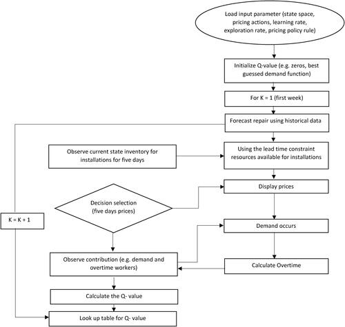
The reinforcement learning algorithm allows us to find the optimal price to maximize the profit gained by installation services, given the number of resources available for installation at a regular wage in week w, as summarized in Figure 2.

Figure 2. Framework of the proposed approach.

Before discussing the dynamic pricing algorithm in procedural form (as presented in Table 1), two essential elements must be introduced: the exploration and learning rates. The absence of perfect prior information concerning the demand model introduces a new component into the dynamic optimization problem, the trade-off between exploration (attempting non-optimal decisions to improve the current policy) and exploitation (choosing the best policy thus far to maximize the expected profit). The longer one learns the demand; the less time is spent exploiting prices that optimize revenue.

Table 1. An online dynamic pricing algorithm for installations using a lead time constraint to determine inventory level.

Step 1: Input parameters: state space, pricing actions, learning and exploration rate, policy rule

Step 2: Initialize $Q(K^I,P);$

For w = 1 (first week)

Repeat for each week $w\to \infty$

Step 3: First stage: Forecast Repair using historical data for a week w

Step 4: Using constraints 1(b) and 1(e) to calculate resources required for maintenance

Step 5: Calculate the resources for installation K^I using $k_t^I=f_t-e_t^M$ $\forall$ t = $1\dots T$

Step 6: For state K^I select an decision P according to the ϵ-greedy (1/w)

(For the neighborhood search, the exploration method follows Table 2) policy π: $K^I\to P$

Step 7: Display prices P

Step 8: Second stage: Observe the actual demand in week w for each t, $d_t^I$ and $d_t^M$

Calculate overtime workers using the observed demand in a week w for each K^I with prices P

$\forall$ K^I at price P: $c(K^I,P)={\sum }_{t=1}^T(d_t^I{p}_t-(o_t^M(k_t^I)+o_t^I(k_t^I)){\lambda }_0)$

Step 9: Third stage: Update Q-values $\forall$ K^I at price P:

$Q(K^I,P)\leftarrow Q(K^I,P)+{\alpha }_w(K^I,P)(c(K^I,P)-Q(K^I,P))$

Step 10: $w\leftarrow w+1$

The algorithm’s objective is to obtain an accurate estimate of the near-optimal policy based on observations during the exploration phase while keeping the exploration rate low to limit revenue loss over this learning phase. The exploration rate (ϵ) that we have chosen is an ϵ-greedy policy at a rate $1/w$ so that the learning progresses as the exploration rate decreases, but becomes fixed once it reaches 0.1 and then remains constant at this rate. This is because the environment may be non-stationary; hence, setting the exploration rate in this manner ensures that a new policy is learned if the environment changes. The learning rate is set in the same way.

The algorithm starts by initializing the Q-values. The following steps are repeated for each episode w. State K^I is the technician’s capacity assigned to instal jobs for day 1 to T in week w. First, the expected number of maintenance jobs is forecast. Then, the number of workers needed to perform the maintenance jobs to meet the regulation (lead time) constraints is calculated and deducted from the total. The pricing decisions P are selected from an ϵ-greedy policy. Then, after observing demand for both services, we calculate the contribution profit for all states K^I for price P. We can calculate the contribution profit for all K^I and not just the state in a week w because demand depends on price P and not on state K^I. Hence we can calculate the overtime work for installation for each state $K^I\in K$ and determine its contribution profit. This significantly reduces the dimensions of the problem, as demand learning in any state can be used to update the values in all other states for that price action. Finally, the Q-values of the state actions are updated, and the process is repeated for the next week. A simple illustration of the calculation can be found in Appendix A.2.

The Q-learning algorithm has many advantages; however, the curse of dimensionality is present in large practical problems. To address this challenge, researchers proposed using linear and nonlinear approximators to estimate the Q-values without needing to visit all state–action pairs (Sutton and Barto, 1998). We try to use the new information learned in the visited state to update other related state-action pairs.

We also introduce smarter exploration by looking at an extension of the algorithm. Let $Q^{*}$ denote the optimal expected Q-value of the state K^I when every pricing and overtime decision is executed in each state infinitely. As randomly exploring the state of pricing policies can be very costly due to non-optimal policies, we now consider an exploration strategy that uses the knowledge of the actions already tried to select future pricing actions. We call this algorithm the Bandit With Neighborhood Search, as summarized in Table 2. We assume a solution of a vector of pricing action $P\in P(K^I)$ and the profit contribution at $c(K^I,P).$ Each solution of $P\in P(K^I)$ has an associated set of neighbors, i.e., the prices near P, a subset N(P) of all the possible pricing policies, $N(P)\subset P(K^I).$ Each solution $P\prime$ $\in N(P)$ can be reached directly by a move operation. The innovation of the neighborhood search is the way that the exploration of pricing actions is selected. The Q-values are updated as represented in Table 1.

Table 2. Neighborhood search Exploration Method.

Step 1: After initial exploration for n weeks

Step 2: Select a starting solution P^now

Step 3: Record the current best-known solution (generating the most profit) by setting

P^best = P^now and define best-profit = $c(K^I,P^{\mathit{best}})$

Step 4: Choose P^next $\in N(P^{\mathit{now}}),$ use local exploration ρ times, and global exploration (1-ρ) times

Step 5: Re-set P^now = P^next if $c(K^I,P)>$ best-profit, perform step 3.

We start with an initial exploration by randomly choosing the pricing action from a discrete price set for n weeks. After n weeks, we use the pricing action that generates the most profit as our starting solution P^now. We then select prices in the neighborhood of the best price solution p^now, ρ (e.g., 0.9) of the time. We update our best solution P^now if the profit contribution with P^next is higher.

5. Optimality conditions and structural results

In this section, we investigate the model’s main features. First, we establish an upper bound on the optimal solution, starting by assuming perfect demand forecasting: hence equation (4)(4) $${\mathbb{E}}^{\pi }\left(\sum _{t=1}^T\left(d_t^I{p}_t-(o_t^M+o_t^I){\lambda }_0\right)\right)$$(4) (4) $${\mathbb{E}}^{\pi }\left(\sum _{t=1}^T\left(d_t^I{p}_t-(o_t^M+o_t^I){\lambda }_0\right)\right)$$(4) simplifies to ${\max }_{p_t}E({\sum }_{t=1}^T{d}_t^I{p}_t).$ The deterministic problem is defined as follows. At the start of the planning horizon, for each day t = 1,…, T, the company has a vector of resources available for installations K^I. Let the finite planning horizon be represented by 0 $\le$ x $\le$ z. Demand at time x is modeled as a vector of rates $d^I(x)=(d_1^I(x),\dots ,d_T^I(x))$ that are a functions $d^I(P,x)$ of a fixed price vector for the entire planning horizon P = $(p_1,p_2,\dots ,p_T).$

We assume that demand and revenue function $r(d^I(x),x)=d^I(x)P$ satisfy regularity assumptions (Gallego and van Ryzin, 1997) and salvages are zero. The price vector P is chosen from a set of allowable prices. We can equivalently view the firm as setting the vector of purchases rates $d^I(x)$ $\in$ f(x), where f(x) is a discrete set of purchase rates, which implies charging a vector of prices $P=P(d^I(x)).$ The firm maximizes the revenue over [0, z], given K^I, denoted as $V(K^I),$ and subject to the capacity constraints, as represented by program (6): (6a) $$\mathrm{ }V(K^I)=\max {\int }_0^{z}r(d^I(x),x)dx\hspace{1em}$$(6a) (6b) $$\begin{array}{c}s\mathit{ubject}to:\\ {\int }_0^z{d}^I(x)dx\le K^I,\hspace{1em}\end{array}$$(6b) (6c) $$\hspace{1em}{d}^I(x)\in f(x),\hspace{1em}$$(6c) (6d) $$\hspace{1em}0\le x\le z.$$(6d)

Moreover, let us define the run-out rate, price vector and revenue, respectively, by $d^{I0},$ P⁰ = $P(d^{I0})$ and $r^0=P^0{d}^{I0}.$ Note that P⁰ is the price at which the firm sells exactly K^I resources. Let $d^{I^{*}}$ be the least maximizer of the revenue function $r(d^{I^{*}})$ = $d^{I^{*}}P(d^{I^{*}}).$ Proposition 5.1 shows the optimal solution for the deterministic case, which is an upper bound on the stochastic case (i.e., Gallego and van Ryzin, 1997).

Proposition 5.1.

The optimal solution to the deterministic problem is d^I = $\min \{d^{I^{*}},d^{I0}\}$, 0 $\le$ x $\le$ z. In terms of price, the optimal policy is $P=P^D=\max \{P^{*},P^0\}$, 0 $\le$ x $\le$ z. Finally, the optimal revenue over the entire horizon is $V(K^I)=\min \{r^{*},r^0\}$.

In Proposition 5.2, we prove that constraint (1e)(1e) $$\mathbb{E}\left(S_t^M\right)\le \overline{L}{\beta }^M\left(e_t^M-\mathbb{E}\left(a_t^M\right)\right),\hspace{1em}\forall t$$(1e) relating to the cumulative stack size for maintenance services can be operationalized in such a way that it is still linear.

Proposition 5.2.

Let l stand for the lag period for which the actual stack is known. Then constraint (1e)(1e) $$\mathbb{E}\left(S_t^M\right)\le \overline{L}{\beta }^M\left(e_t^M-\mathbb{E}\left(a_t^M\right)\right),\hspace{1em}\forall t$$(1e) is equivalent to $e_t^M\ge \frac{S_{(t-l)}^M}{\overline{L}{\beta }^M}+\mathbb{E}(a_t^M).$

Currently, the firm manages the resources for maintenance and installation separately. There is a fixed number of technicians assigned to maintenance $e_t^M$ and to installations $e_t^I,$ in each day t, we continue by analyzing the effectiveness of resource management under these conditions. The number of technicians is optimized at a fixed price p and the overtime work on maintenance equals $o_t^M=\max \{S_t^M-\overline{L}{\beta }^M(e_t^M-a_t^M),0\}.$ In Proposition 5.3, we show that the joint management of resources increases profit contribution, even when the installation price is fixed. This is the first step in improving how the technicians are currently managed, focusing on the real-world scenario of scarce resources.

Proposition 5.3.

Let the expected contribution to profit be represented by (4), with a fixed price p_t = p. Additionally, let the resources be scarce at day t so that one of the resources is a binding constraint. In contrast, the other one has a slack capacity, as defined by constraints (1b)(1b) $$\begin{array}{c}s\mathit{ubject}to:\\ \mathbb{E}\left(d_t^M\right)\le {\beta }^M\left(e_t^M-\mathbb{E}\left(a_t^M\right)\right),\hspace{1em}\hspace{1em}\hspace{1em}\forall t\end{array}$$(1b) and (1c)(1c) $$\mathbb{E}\left(d_t^I\right)={\beta }^I\left(e_t^I-\mathbb{E}\left(a_t^I\right)\right),\hspace{1em}\hspace{1em}\forall t$$(1c) . The joint management of resources increases profit contribution.

Another critical issue central to our analysis is the maintenance regulation, which translates to the required service quality controlled using the maximum lead time. In Proposition 5.4, we analyze the effect of a decrease in the maximum lead time, due either to regulation or the willingness of the company to improve service quality, on the number of technicians required to be available on the days when resources are scarce. We prove that the increase in the expected number of available technicians is directly proportional to the decrease in the maximum lead time.

Proposition 5.4.

Let the maximum lead time $\overline{L}$ be a binding constraint, such that $\mathbb{E}(S_t^M)=\overline{L}{\beta }^M(e_t^M-\mathbb{E}(a_t^M))$ at time t. A decrease in this maximum lead time, $\overline{L^{\prime }}\le \overline{L}$, for any $\mathbb{E}(S_t^M)$, increases the required number of technicians available at t by$$\frac{e_t^{M^{\prime }}-\mathbb{E}\left(a_t^M\right)}{e_t^M-\mathbb{E}\left(a_t^{M^{\prime }}\right)}=\frac{\overline{L}}{\overline{L^{\prime }}}.$$

On the other hand, this also means that a better allocation of resources may be attained if the company can reduce the number of jobs in the queue when resources are scarce. It seems that the maintenance service queue can decrease if the resources are reallocated, so more technicians are available on low-demand days if there is an overall capacity slack. For this reason, in Proposition 5.5 we prove that, even when service prices are fixed, a decrease in the maximum lead time, if accommodated by reallocating available resources from low to high demand periods, is not detrimental to the contribution to profit, i.e., if the regulator, or the company, decide to increase the quality of the maintenance service, this may be achieved without compromising profitability. This result also implies that, in general, due to the fixed cost of the available workforce, there are multiple solutions to the problem.

Proposition 5.5.

Let the service prices be fixed so that the profit contribution is equal to ${\sum }_t^T(d_t^{I}p-(o_t^M+o_t^I){\lambda }_0)$ and let us define a partition such that t₀ stands for days where capacity is more than enough to meet demand and t₁ stands for days where capacity is fully used to meet the required maximum lead time. A decrease in this maximum lead time, so that $\overline{L^{\prime }}\le \overline{L}$, has no impact on the profit contribution if $\sum _{t0}(e_{t_0}^M-\mathbb{E}(a_{t_0}^M)-e_{t_0}^{M^{\prime }}+\mathbb{E}(a_{t_0}^{M^{\prime }}))\ge \sum _{t1}(e_{t_1}^{M^{\prime }}-\mathbb{E}(a_{t_1}^{M^{\prime }})-e_{t_1}^M+\mathbb{E}(a_{t_1}^M)).$

Next, in Proposition 5.6, we extend this result by proving that the joint management of resources using dynamic pricing for installations increases profit contribution and allows better management of resources by decreasing overtime costs.

Proposition 5.6.

If the firm manages the resources jointly, and expected demand is seasonal, i.e., for at least one time $t_0\ne t,\mathbb{E}(d_{t_0}^I)\ge \mathbb{E}(d_t^I)$, then dynamic pricing increases profit contribution.

We now re-address the issue of service quality, analyzed in Proposition 5.4, in the context of its interaction with dynamic pricing. In Proposition 5.7, we show that dynamic pricing of installation services increases profit contribution when resources are scarce. If the price increase reduces the demand for services large enough to free some technicians, then it also increases maintenance quality.

Proposition 5.7.

Let the constraint on lead time be binding, such that, $\mathbb{E}(S_t^{\mathit{j}})=\overline{L}{\beta }^{\mathit{j}}(e_t^{\mathit{j}}-\mathbb{E}(a_t^{\mathit{j}}))$ for $j=I,M$ at time t. Dynamic pricing of installation services at time (a) t increases $\mathbb{E}(d_t^I{p}_t-(o_t^M+o_t^I){\lambda }_0)$, and (b) if $\mathbb{E}(d_t^I(p_t))<k_t^I$, decreases the maintenance lead time to$$L_t^M=\frac{S_t^M}{{\beta }^M\left(e_t^M-a_t^M+\max \left(k_t^I-\mathbb{E}\left(d_t^I(p_t)\right),o_t^M\right)\right)}.$$

It follows from Proposition 5.7 that the firm can improve service quality, increase revenue, and decrease costs by introducing dynamic pricing when resources are scarce. The condition $\mathbb{E}(d_t^I(p_t))<k_t^I$ guarantees that the reduction in demand for installation services at time t needs to be large enough to free up resources to be used in maintenance. The reduction of lead time only occurs if the resources freed for maintenance are greater than the overtime technicians hired, i.e., $\max (k_t^I-\mathbb{E}(d_t^I(p_t)),o_t^M),$ otherwise, there is a reduction of costs due to less overtime work, but the lead time remains the same.

6. A case study

This section illustrates our algorithm with a case study analyzing the company’s pricing policies. We use the following parameters:

1. The reference price is indexed to 100. Based on the historical data, the average demand at this fixed price is around 6600 installation jobs. The price set considered in the simulation is {105, 104, 103, 102, 100, 98, 96, 95}. As price differentiation is regulated, we assume the service charges should not vary more than 10%.

2. The cost of overtime work is 120 per day (when compared with 60 for the regular pay rate).

3. The productivity parameter is estimated using historical data and is equal to 2.8 and 2.5 jobs per technician on any given day for maintenance jobs and installations, respectively.

4. Lead times are between 1 and 1.5 days during the weekdays. Thus, the target for the maximum lead time is set at 1.5.

5. As the underlying functional relationship between price and demand is unknown, we have used both linear and nonlinear functions in these simulations, with stochastic parameters, to compare the effectiveness of the algorithms. Initially, we generate the data using a steep and flat demand function, including interactions between days. ($\forall$ t, $j\ne t,d_t^I=20000-134.75p_t-\sum _{j}30(p_t-p_j$) and $\forall$ t $j\ne t,d_t^I=13150-65.75p_t-\sum _{j}30(p_t-p_j$).

6. The installation resources can vary daily from 2300 to 2900 based on historical demand data for maintenance.

We first examine the performance of the learning algorithms. Our initial Q-values can be set using sensible demand functions from market research to avoid loss at the initial exploration stage. If we assume a demand structure (e.g., linear) and this is the actual demand structure, we can arrive at an optimal policy quite quickly. If we assume a demand structure and it is the wrong structure (e.g., if the actual design was exponential and we took it to be linear, for example), then we will lose revenue because the model has been misspecified (for a detailed discussion of this point see, e.g., Besbes and Zeevi, (2009)). We refer to this as a parametric misspecified model.

Reinforcement learning is used to determine the dynamic pricing policy for installations. We compare our model-free approach to parametric learning algorithms to understand the advantages and limitations of learning algorithm approaches for our problem. We consider the following experimental set up, where the true demand is $d_t^I=\mu -{\theta }_t{p}_t-\sum _j{\theta }_j(p_t-p_j)$ and μ is the customer arrival rate drawn randomly from a uniform distribution $[19000,21000],$ θ_t = 134.75 and θ_j = 30. The simulated demand can vary in the range [9399, 4551], as it depends on the random customer arrival and the prices selected for service each day.

The parametric misspecified model is defined as $\mu e^{{\beta }_t{p}_t+\sum _j{\beta }^{\mathit{j}}(p_t-p_j)},$ for all j $\ne t.$ The demand is assumed to follow an exponential model, and the algorithm learns its parameters from actual data. As the real data, in reality, is a linear function of price, the learned model is misspecified. For this reason, an exponential, misspecified model is not expected to converge to the optimal policy.

The average percentage difference in contribution measures the performance of the four algorithms compared to the fixed price policy. We have run 1000 experiments for each algorithm, and the results are recorded in Table 3.

Table 3. Profit contribution under four learning algorithms compared with fixed pricing.

Algorithm	Percentage Difference
Bandit	2.3
Bandit (neighborhood search)	3.2
Parametric(well structured)	4.0
Parametric(misspecified)	−0.5

From Table 3, we can see that the parametric algorithm outperforms both these algorithms when the assumed model is consistent with the true demand function. Otherwise, the parametric algorithm makes less contribution compared with the fixed price policy.

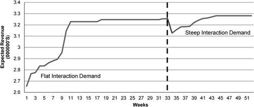
The reinforcement learning algorithm can learn in a changing environment. As illustrated in Figure 3: the initial demand was a flat demand with interaction; after the 32-week mark, the demand for installations becomes more price sensitive. For this reason, the current pricing policy is not optimal, as it results in a lower contribution, given the new demand. Then by updating the Q-values through interaction with the new demand function, the algorithm finds a better pricing policy.

Figure 3. Learning the Q-value for a changing demand.

When the parametric demand model is well specified, a large amount of data is not required to learn the parameters in the demand model, similar to Besbes and Zeevi (2009)). When the demand structure is unknown, more exploration and data are needed to learn the optimal policy, even as much as 1000 weeks of data. The service provider works nationally around the UK, and the data in similar regions can be pooled to learn the value of state and action pairs. The algorithm starts with the best-guessed Q-values (using the demand they believe is the genuine demand) so that prices are set more proactively until the near-optimal policy is learned. The Q-value learns the value of the optimal policy, independently of the functional form of the demand, and considers (implicitly) the availability of workers and interaction between the pricing policies for the different days.

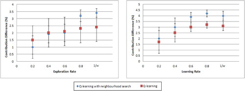
We explore different learning and exploration rates for the bandit algorithms. The Q-values are set to zero, and for the first 10 weeks, we set the initial learning and exploration rates at 0.2, 0.4, 0.6, and 0.8. After 10 weeks, the exploration rate is reduced to a minimum of 0.05. The rate of $1/w$ decreases as the number of weeks increases. When comparing different learning rates, the exploration rate is fixed to $1/w,$ and when varying the exploration rate, the learning rate is set to $1/w.$ Figure 4 shows that the bandit algorithm using neighborhood search performs better than the bandit algorithm when the initial rate of exploration is high. Otherwise, it may perform worse, because it may get trapped into exploring actions around a sub-optimal solution. Also, when the initial learning rate increases, we are likely to find a near-optimal pricing policy faster.

Figure 4. Impact of exploration and learning on profit contribution.

Next, simulation experiments are used to compare the performance of both models: the proposed model of joining resources for installation and maintenance and applying dynamic pricing to the former, compared to using two separate teams of resources for both services and considering a fixed pricing policy for installation services. The models are tested on data from October 1, 2019 to March 26, 2020. The effects of forecasting errors on optimal pricing policies are also analyzed. The number of workers required to meet service-level agreements for the maintenance service is under-forecast and over-forecast by 5%. The error of under-forecasting results in fewer workers being assigned to carry out maintenance jobs than required. In this case, the dynamic pricing policy with the under-forecasting error assigns some maintenance capacity to installations. Then, additional workers are needed for overtime to meet the service-level agreement for the maintenance service. On the other hand, when the number of workers required for the maintenance service is over-forecast, fewer workers are assigned to installations compared with a perfect forecast.

Table 4 illustrates the percentage increase in profit contributions for dynamic vs. fixed pricing under different demand functions for installation services. We used 1000 simulations to compute the 95% confidence intervals. The four demand functions considered are: (i) flat, (ii) flat with interactions between days, (iii) steep, and (iv) steep with interactions between days.

Table 4. 95% Confidence intervals for the percentage increase in contribution for dynamic vs. fixed pricing.

Parameter	Level	Perfect Forecast	Over- Forecast	Under- Forecast
Demand	(i) Flat	(3.63, 3.78)	(2.53,2.67)	(1.2,1.4)
	(ii) Flat Interactions	(4.12,4.28)	(3.1,3.21)	(1.91,2.10)
	(iii) Steep	(4.42,4.5)	(3.31, 3.45)	(2.60,2.80)
	(iv) Steep Interactions	(4.8,4.91)	(3.30,3.40)	(2.10,2.13)

As expected, the steep demand function results in a higher percentage of contribution increase compared with the flat demand. For the flat and steep demand with the interaction between days, there is a higher contribution increase compared with their demand function without interaction, because the interaction effect can help shift some demand from one day to another. All four demand functions significantly improve contribution compared to the fixed pricing strategy.

Table 4 also reports the effect of systematic forecasting errors on the profit contribution. A 5% under-forecast or over-forecast maintenance job can significantly affect the profit generated by the dynamic pricing policies. As expected for all four demand functions, the perfect forecast has the most substantial positive contribution. An over-forecast of maintenance also increases the profit contribution compared with fixed pricing. In this case, even though there is no increase in overtime cost, as the salaries are given, it leads to a rise in resources allocated to installations which, under high-demand days for maintenance, increases the use of overtime work.

Finally, we have studied the effects of the lead time for maintenance services on the profit contribution to better explain the effectiveness of dynamic pricing. The results are summarized in Table 5. The confidence intervals show the difference in contribution from increasing the lead time requirement. For example, for a perfect forecast of maintenance demand with a lead time of 3 days, the increase in contribution compared with a fixed pricing policy with a lead time of 1.5 is between 4.4 and 4.8%. Our results indicate that dynamic pricing is less effective as the lead time for maintenance jobs increases, because the maintenance workforce can manage its demand more efficiently without needing installation workers. Increasing the lead time from 1.5 to 3 days significantly impacts the profit contribution, but deteriorates the quality of service. Increasing the lead time to 5 days does not significantly increase profit and further deteriorates service quality.

Table 5. 95% Confidence intervals for the percentage increase in contribution for different lead times.

Parameter	Level	Perfect Forecast	Over- Forecast	Under- Forecast
Lead time (days)	3	(4.4,4.8)	(4.1,4.3)	(4.2,4.4)
	5	(4.9,5.2)	(4.2,4.4)	(4.3,4.5)

Table 6 shows an example of dynamic pricing. The average service charge is indexed to 100. We analyze how the customers can get discounts or be charged more throughout the week to manage demand. As shown, with dynamic pricing for a Flat demand on a Monday, the premium charged is 5%, and on a Thursday, the firm gives a discount of 3.5%. The optimal pricing policy for each day of the week is computed under different demand regimes. For example, the flat demand function offers price discounts on Wednesday (1.5%), Thursday (3.5%), and Friday (5%). The importance of including the interaction effect can be seen in the difference in prices: by considering the possible cannibalization effect between the different days, the price changes decrease. We can see that under flat demand functions, the firm provides discounts, and the firm learns to have some days with no discount under steeper ones.

Table 6. Premiums charged and discounts as percentage of the fixed price.

Demand	Monday	Tuesday	Wednesday	Thursday	Friday
Flat	5.0	4.0	−2	−4	−5.0
Flat Interactions	2.0	2.0	0.0	0.0	−2.0
Steep	5	5	0.0	0.0	0.0
Steep Interactions	5	4.0	2	0.0	0.0

7. Conclusion

This article is the first to explore the interplay of shared resources and dynamic pricing, considering two field service operations, and solving the problem using reinforcement learning.

The main managerial results show that

1. Dynamic pricing and the joint management of resources increase profitability by around 3%.

2. Regulation of the service window is needed to maintain the service quality. In the numerical experiments, we observe that an increase from 1.5 to 3 days in the maximum lead time (deteriorating service quality) increases profit contribution. Still, an additional boost of the maximum lead time to 5 days has no statistically significant impact on profit.

3. Under certain conditions, dynamic pricing of installation services can decrease the maintenance lead time.

4. Underestimation of demand is more detrimental to profit than overestimation. Concerning the usefulness of improving demand forecasting accuracy for the overall efficiency of managing the resources, we have shown that under (over) estimation of demand leads to higher (has no impact on) overtime costs.

We have shown that using dynamic pricing and flexible resources as strategies can help maintain quality levels while increasing profit for field service operations. Reinforcement learning has been used to find near-optimal pricing policies when there are both demand and capacity uncertainties.

In many industries, firms are unsure about trusting black-box algorithms such as reinforcement learning approaches. For this reason, simpler models may be preferred, but these are disadvantageous if relying on assumptions that are simplifications of real-world complexity. The main advantages of using a reinforcement learning approach compared to stochastic integer-linear programming, for example, in our problem, are as follows:

1. The relationship between the prices and demand is not linear, and its functional form unknown and unobservable.

2. We must make unrealistic assumptions that lead to non-optimal pricing policies.

3. If the demand function changes, the Q-learning algorithm can adapt to finding the new optimal policy, as illustrated in Figure 3.

4. From the learning algorithm, we infer the optimal dynamic pricing policies represented as look-up tables, which is a handy tool for managers.

Future work will consider the geographical movement of engineers to relax the assumption of fixed number of engineers, where engineers can be moved between patches (currently, each patch manages the engineers in their region) in proximity. Additionally, we would like to study non-stationary environments in which demand and pricing are time-dependent.

Additional information

Notes on contributors

Rupal Mandania

Rupal Mandania is a Lecturer in Management Science at the School of Business & Economics, Loughborough University. She holds a bachelor’s degree in mathematics from Leicester University, MSc in statistics from Nottingham University, and PhD (sponsored by British Telecom) in operational research from Warwick University. Her main research interest area is in revenue management and operations planning and scheduling in production and logistics.

Fernando S. Oliveira

Fernando S. Oliveira is professor of Business Analytics and Sustainability and Head of Business Analytics, Circular Economy and Entrepreneurship Department at the University of Bradford School of Management. He holds a PhD in Management Science and Operations from the London Business School, an MSc in Artificial Intelligence, and a Licenciatura in Economics from the University of Porto, Portugal. Before joining the University of Bradford, Fernando was Associate Professor in Operations Management and Analytics at the Auckland Business School and Professor at ESSEC business school. He has held several visiting positions, including visiting Professor of Operations Management and Analytics at the National University of Singapore and visiting researcher at Johns Hopkins. He has received two prizes for his publications, the Prix Académique SYNTEC, and the European Journal of Operational Research best paper award. His research has been published in top international journals, including Decision Sciences, Energy Economics, European Journal of Operational Research, Informs Journal on Computing, International Journal of Production Economics, Omega, and Operations Research. He is on the International Journal of Data Science editorial board, the International Journal of Business Analytics area editor, and the associate editor of Energy Systems. His teaching and research interests are in applications of artificial intelligence to managerial problems in supply chain management and, more specifically, healthcare, energy markets, and quantitative risk management.

References

- Asheralieva, A. and Niyato, D. (2020) Distributed dynamic resource management and pricing in the IoT systems with blockchain-as-a-service and UAV-enabled mobile edge computing. IEEE Internet of Things Journal, 7(3), 1974–1993.
- Besbes, O. and Zeevi, A. ( 2009) Dynamic pricing without knowing the demand function: Risk bounds and near-optimal algorithms. Operations Research, 57(6), 1407–1420.
- Bish, E.K. and Suwandechochai, R. (2010) Optimal capacity for substitutable products under operational postponement. European Journal of Operational Research, 207(1), 775–783.
- Bondoux, N., Nguyen, A.Q., Fiig, T. and Acuna-Agost, R. ( 2020) Reinforcement learning applied to airline revenue management. Journal of Revenue and Pricing Management, 19, 332–348.
- Ceryan, O., Sahin, O. and Duenyas, I. (2013) Managing demand and supply for multiple products through dynamic pricing and capacity flexibility. Manufacturing and Service Operations Management, 5(1), 86–101.
- Chan, L.M.A., Shen, Z.J.M., Simchi-Levi, D. and Swann, J.L. (2004) Coordination of Pricing and Inventory Decisions: A Survey and Classification, Kluwer Academic Publisher, Boston, MA.
- Chen, M. and Chen, Z-L. (2015) Recent developments in dynamic pricing research: Multiple products, competition, and limited demand information. Products and Operations Management, 24(5), 704–731.
- Chen, M. and Chen, Z-L. (2018) Robust dynamic pricing with two substitutable products. Manufacturing and Service Operations Management, 20(2), 249–268.
- Chen, X. and Simchi-Levi, D. (2012) Pricing and Inventory Management. Oxford University Press, Oxford, UK.
- Cheng, Y. (2009) Real-time demand learning-based Q-learning approach for dynamic pricing in e-retailing setting, in International Symposium on Information Engineering and Electronic Commerce, pp. 594–598, IEEE Conference, Ternopil, Ukraine.
- Chod, J. and Rudi, N. (2005) Resource flexibility with responsive pricing. Operations Research, 53(3), 532–548.
- den Boer, A.V. (2015) Tracking the market: Dynamic pricing and learning in a changing environment. European Journal of Operational Research, 247(3), 914–927.
- Ding, Q., Kouvelis, P. and Milner, J.M. (2007) Dynamic pricing for multiple class deterministic demand fulfillment. IIE Transactions, 39(11), 997–1013.
- Gallego, G. and van Ryzin, G.J. (1997) A multi-product dynamic pricing problem and its applications to network yield management. Operations Research, 45, 24–41.
- Goyal, M. and Netessine, S. (2010) Volume flexibility, product flexibility or both: The role of demand correlation and product substitution. Manufacturing & Service Operations Management, 13(2), 180–193.
- Hanke, J.E. and Wichern, D.W. (2005) Business Forecasting (8th Edition), Pearson, Prentice Hall, NJ.
- Hariharan, S., Liua, T. and Shenm, Z.J.M. (2020) Role of resource flexibility and responsive pricing in mitigating the uncertainties in production systems. European Journal of Operational Research, 284(2), 498–513.
- Kim, B.G., Zhang, Y., Van Der Schaar, M. and Lee, J.W. (2016) Dynamic pricing and energy consumption scheduling with reinforcement learning. IEEE Transactions on SmartGrid, 7, 2187–219.
- Kastius, A. and Schlosser, R. (2021) Dynamic pricing under competition using reinforcement learning. Journal of Revenue and Pricing Management, 21, 50–63.
- Luong, N.C., Wang, P., Dusit, N., Wen, Y. and Han, Z. (2017) Resource management in cloud networking using economic analysis and pricing models: A survey. IEEE Communications Surveys and Tutorials, 19(2), 954–1001.
- Lus, B. and Muriel, A. (2009) Measuring the impact of increased product substitution on pricing and capacity decisions under linear demand models. Production and Operations Management, 18, 95–113.
- Maestre, R., Duque, J., Rubio, A. and Arevalo, J. (2019) Reinforcement learning for fair dynamic pricing. Intelligent Systems and Applications, 120–135.
- Misra, K., Schwartz, E.M. and Abernethy, J. (2019) Dynamic online pricing with incomplete information using multi-bandit experiments. Marketing Science, 38(2), 226–252.
- Rana, R. and Oliveira, F.S. (2015) Dynamic pricing policies for interdependent perishable products or services using reinforcement learning. Expert Systems with Applications, 42(1), 426–436.
- Sharghivand, N., Derakhshan, F. and Siasi, N. (2021). A comprehensive survey on auction mechanism design for cloud/edge resource management and pricing. IEEE Access, 9, 126502–126529.
- Sutton, R. and Barto. A.G. (1998) Reinforcement Learning. The MIT Press, Cambridge, MA.
- Vicil, O. (2021) Inventory rationing on a one-for-one inventory model for two priority customer classes with backorders and lost sales IIE Transactions, 48(10), 955–974.