Uncovering illicit supply networks and their interfaces to licit counterparts through graph-theoretic algorithms

Abstract

The rapid market growth of different illicit trades in recent years can be attributed to their discreet, yet effective, supply chains. This article presents a graph-theoretic approach for investigating the composition of illicit supply networks using limited information. Two key steps constitute our strategy. The first is the construction of a broad network that comprises entities suspected of participating in the illicit supply chain. Two intriguing concepts are involved here: unification of alternate Bills-of-materials and identification of entities positioned at the interface of licit and illicit supply chain; logical graph representation and graph matching techniques are applied to achieve those objectives. In the second step, we search for a set of dissimilar supply chain structures that criminals might likely adopt. We provide an integer linear programming formulation as well as a graph-theoretic representation for this problem, the latter of which leads us to a new variant of Steiner Tree problem: Generalized Group Steiner Tree Problem. Additionally, a three-step algorithmic approach of extracting single (cheapest), multiple and dissimilar trees is proposed to solve the problem. We conclude this work with a semi-real case study on counterfeit footwear to illustrate the utility of our approach in uncovering illicit trades. We also present extensive numerical studies to demonstrate scalability of our algorithms.

Keywords:

• Illicit trade
• bill-of-materials
• Steiner tree problem
• dissimilar trees
• illicit supply chains
• generalized group Steiner tree

1. Introduction

Illicit trades refer to businesses that generate revenue through illegal and unethical activities at the expense of the economy, society, and environment (World Economic Forum, 2012). From the perspective of an illicit trader, their operations are fraught with a number of challenges, precipitated by the absence of supporting infrastructure as well as the constant risk of exposure (Crotty and Bouche, 2018). However, illicit trade volume has surprisingly maintained an upward trend, causing huge concerns across the world (Mashiri and Sebele-Mpofu, 2015; Coke-Hamilton and Hardy, 2019). There are two perspectives to explain this phenomenon: demand and supply. The demand perspective implies the existence of nontrivial demand for illicit product consumption, as well as for involvement in illicit trades. The supply viewpoint, on the other hand, indicates the capability of illicit traders to supply their products without accruing significant monetary or personnel loss. Motivated by the latter perspective, this research aims to unravel the intricacies of illicit supply networks using a graph-theoretic approach.

Similar to their licit counterparts, illicit trades operate through a formal/informal network of suppliers and manufacturers. However, the two supply chains differ significantly in certain aspects (for a detailed review, see Anzoom et al. (2022a)). One important differentiating feature is their levels of visibility. Illicit trades are innately clandestine, and hence, need all parts of their operations to remain undetectable, even under scrutiny. This raises the difficulty level for law enforcement agencies to track any entities participating in the illicit supply chain operations. Interestingly, not all organizations in an illicit supply chain need to be illegal (see Figure 5 in Anzoom et al. (2022a)). As an example, let us consider the supply chain for counterfeit shoes, which is one of the most frequently confiscated products worldwide (22% of global seizures by value) (OECD and European Union Intellectual Property Office, 2019). To manufacture a shoe, the counterfeiter requires a sole, which is in fact a legal product that can be acquired from legitimate manufacturers. The illicit traders may formally purchase soles from a legally operating company or corrupt some personnel to smuggle them out of their facility. Regardless of the sourcing strategy, the supplier facilities involved (either knowingly or unknowingly) are part of both licit and illicit supply chain operations. We define these as interface points of licit and illicit supply networks; i.e., entities where licit and illicit supply networks intertwine. Identification of these points will reveal information about the illicit supply chain, thus increasing its visibility. Hence, one topic of interest in this research is to identify potential interface points.

Knowledge of the interface points allows us to investigate the possible topologies of the illicit supply network. In traditional supply network design, one generally prioritizes cost/risk minimization (efficiency); see, e.g., Chauhan et al. (2006) and Pan and Nagi (2013). The same objectives may prove unsuitable for illicit traders, as they are more focused on effectiveness (execution without exposure). Hence, the search for a minimum-cost network design may be short-sighted. Instead, we can account for effectiveness by extending the search to the k-best network topologies. However, in the case of small k, one runs the risk of deriving highly similar networks and failing to account for any solution diversity. Thus, our interest shifts to obtaining a set of efficient, yet dissimilar, network structures. This, along with the interface point identification, form the core of our research endeavor.

In order to formulate and solve this problem, we draw upon knowledge from multiple disciplines, primarily from product design, production systems, and graph theory. The formulation phase focuses on creating the suspected illicit supply network using limited information. This involves the unification of alternate Bills-of-Materials (BOMs) of the illicit product, and its conversion into a generalized supply network structure. An important task here is the identification of interface points, which we accomplish through a graph (nodal) matching between the licit and illicit (base) network. To obtain the dissimilar supply network structures, we propose approaches based on mathematical programming and graph-theoretic algorithms. For the latter, we associate the problem with a new variant of the Steiner Tree problem and devise an algorithm using ideas from Murty’s k-best assignment problem (Murty, 1968). We also add a semi-real case study on counterfeit footwear trading, which was previously mentioned as a major domain of illicit trades (OECD and European Union Intellectual Property Office, 2019). Despite the unavailability of real data for some attributes, this is still useful for illustrating how our approach can be applied in a practical setting, as well as highlighting the insights offered from the outputs.

We anticipate that this research will make contributions from both societal and technical standpoints. Our proposed methodology to track illicit supply networks uses limited and affordable information, making it beneficial to all stakeholders in the fight against illicit trades. Additionally, identifying interface points can expose the vulnerabilities within licit supply networks and create awareness across business organizations and governing agencies. Finally, obtaining a set of dissimilar supply network structures increases the capability of law enforcement agencies in deterring illicit trades while limiting their investigation/surveillance efforts. It also allows for the identification of the crucial members of the supply network (entities that appear frequently in the diverse optimal set). From a technical perspective, our research also offers several novelties. We begin with approaches proposed for BOMs unification and supply network formation; they are unique and improve on existing methodologies in terms of representing variants. En route to the solution of uncovering illicit supply chains, we propose a new variant of the Steiner Tree problem, the Generalized Group Steiner Tree Problem. Although we relax/modify several of its assumptions to solve our problem within the realm of illicit trades, the generalized form remains an interesting problem. The identification of dissimilar trees itself is an inadequately studied problem in graph theory, which we formulate and solve.

This article is organized as follows. Section 2 provides a review of the relevant concepts and prior research. Section 3 focuses on the formation of input graphs for our problem, whereas Section 4 provides a formal discussion on the problem itself. Section 5 re-frames the problem in graph-theoretic perspective and provides an algorithmic approach to derive the solution. The efficacy of these approaches are demonstrated on the case-study in Section 6, along with numerical analysis. Finally, Section 7 concludes the discussion with key takeaways from this research and offers future avenues to explore.

2. Literature review

2.1. Detection of illicit supply networks

The study of illicit supply networks is a broad and multi-disciplinary research domain. Researchers from diverse backgrounds have sought to demystify the clandestine supply chain from their respective viewpoints (readers interested in a deeper understanding of these works are encouraged to study the review article by Anzoom et al. (2022a)). Our research endeavor for this article falls under the subcategory of discovering or detecting illicit supply networks. The existing literature on this issue is largely focused on specific components of the supply network, e.g., identification of illegal products, money laundering, smuggling route detection, among others (Sin and Boyd, 2016; Magliocca et al., 2019; Farrugia, 2020). In comparison, few works have aimed to analyze the whole supply chain. A reason behind this phenomenon could be the extreme difficulty associated with tracking the affiliated facilities/entities. A limited number of research works have attempted to characterize illicit facilities (Crotty and Bouche, 2018; Zhao, 2019) for specific trades, whereas others have addressed the issue by considering regions as network vertices (Meneghini et al., 2020; González Ordiano et al., 2020). Another important aspect that has not received sufficient attention is the sourcing operations of illicit traders. As mentioned, not much information is available on the characteristics of the supplier facilities (Zhao, 2019). However, researchers have focused on the parts/materials that are sourced, especially in the case of fire arms trafficking. Their interest is specifically focused on parts with dual-use characteristics, i.e., ones that can be used for both military and civilian purposes (Micara, 2012). Criminals use corruption and treachery to procure these commodities (Albright et al., 2010). There exist trading restrictions on some raw materials to prevent such incidents, but others are legally tradable and thus vulnerable to illegal sourcing. This also opens up the possibility of tracking or shortlisting the supplier entities (interface points) in the illicit supply network. Our research addresses this issue by utilizing BOMs of the illicit product to identify these organizations.

2.2. Unification of BOMs

A Bill-of-Materials (BOM) provides a catalog of all the components and parts required to produce a single unit of a finished product with particular attention to the hierarchical relationships between different components (Jiao et al., 2000). Multiple BOMs may exist for a single product, given the availability of alternate materials and/or manufacturing processes. Each associated BOM represents a variant design of the original product and thus bears high similarity with others. A well-established approach for generalizing these variant BOMs is to merge them into a Generic Bill-of-Materials (GBOM) (Hegge and Wortmann, 1991), a parameter-constrained structure where certain parameter specifications lead to distinct variant BOMs (Romanowski and Nagi, 2004; Zhu et al., 2007). However, it does not allow for the simultaneous representation of multiple variant BOMs, barring instant visibility of all parts/materials that may flow across the supply chain. We thus require a unification methodology that facilitates such a representation. Logical graphs (e.g., AND-OR, AND-XOR) are good candidates for this purpose (Wedekind and Muller, 1981). Another relevant tool is the Equivalence Class Feature Diagram, which has applications in graph-based variability modeling (Carbonnel et al., 2019). It extends the traditional feature set (AND, OR, XOR) with additional representation capabilities (e.g., mutual exclusivity). In this research, we draw inspiration from these techniques to define a unification methodology for the alternate BOMs. We additionally note that past work in GBOM Romanowski and Nagi, 2004; Romanowski et al. 2006) was conducted from a product design perspective, and there is very little work that attempts to take this formulation forward to the supply chain dimension. Thus, we use the unified BOM to define a generalized version of the supply chain that incorporates all possible network configurations.

2.3. Steiner tree and its variations

The Steiner Tree Problem (STP) is a well-established problem in graph theory and combinatorial optimization, with applications in a wide variety of fields (Hwang and Richards,1992; Ljubic, 2021), including (legal) supply chains (Guanghua and Zhanjiang, 2010; Han et al., 2014)). Formally, the STP looks for a minimum-cost tree that spans a set of terminal nodes $T\subseteq V$ in an undirected graph $G=(V,E).$ The difficulty of the problem stems from the fact that the tree may or may not include additional (Steiner) nodes in $S=V\setminus T.$ The STP is NP-hard in terms of both exact and approximate solution (Chlebık and Janka Chlebıkova, 2008).

Over the years, researchers have proposed multiple variants of STPs (Hauptmann and Karpinski, 2015) Among these, the Group Steiner Tree Problem (GSTP) is of particular interest to our research (Garg et al., 2000). Here, the problem setting includes a collection of mutually exclusive groups of nodes denoted by $S_1,\dots ,S_n\subseteq V$ in the graph, and requires the presence of at least one node from each group in the identified Steiner tree. In essence, the GSTP is a generalized form of the STP, and thus it is also NP-hard (Ihler, 1991). In this research, we uncover a use-inspired new generalization of the GSTP, where not all groups are required to be spanned by the optimal tree, but are held together by other relational constraints. To the best of our knowledge, this is new. This affords us the opportunity to contribute to the general corpus of knowledge on Steiner trees through our research (see Section 5).

Another research gap we intend to address is the incorporation of dissimilarity in our search for multiple Steiner trees. Although researchers have studied the extraction of the k-best Steiner trees from a graph, none of the previous work has considered the notion of dissimilarity (Chudak et al., 2004; Kim et al., 2013). A relevant research topic is the Steiner Tree Packing problem (DeVos et al., 2016), where one looks for the maximum number of pairwise disjoint trees. In contrast, our interest lies in defining a more flexible dissimilarity metric, whose incorporation will lead to a set of Steiner trees with desired properties. For further insight, the next subsection offers a brief review of relevant strategies used for a different, yet relevant, network topology: paths.

2.4. Extraction of dissimilar network topology

To the best of our knowledge, there does not exist any prior work on identifying dissimilar trees within a network. In fact, dissimilarity/diversity rarely plays a role in the extraction of other graph structures, except for paths. This inclusion (dissimilarity into path problems) eventually led to the creation of the Dissimilar/Alternate Path problem which is a well-known problem in graph theory and logistics management (Akgun et al., 2000; Carotenuto et al., 2004). Over the past years, researchers have proposed several approaches to address this problem. Most of these chose spatial distance (Dell’Olmo et al., 2005) and/or number of common elements (nodes/edges) (Moghanni et al., 2022) as the measure of path dissimilarity. Since topological variation in supply networks depends on the elements included, the second dissimilarity measure is better suited to our cause.

Although there exist mathematical programming approaches for solving the Dissimilar Path Problem (Moghanni et al., 2022), the majority of solutions are algorithmic in nature (Dell’Olmo et al., 2005; Chondrogiannis et al., 2018; Gbadamosi and Aremu, 2020). Availability of established algorithms (single and k-shortest path) as subroutines may have impacted this decision (Johnson et al., 1993; Gbadamosi and Aremu, 2020). We aim to adopt a similar approach for our research, i.e., use ideas from Minimum Cost Tree algorithms to derive dissimilar trees. As for the problem objective, the literature notes use of both cost minimization (Johnson et al., 1993) and dissimilarity maximization (Moghanni et al., 2022). However, our goal is to develop a mechanism for extracting a set of cost-efficient trees satisfying a pre-specified minimum level of dissimilarity. To achieve this, we set cost minimization as the sole objective and employ dissimilarity as a parameterized constraint.

3. Problem setup

A key assumption in our research is the availability of credible information on both licit and illicit supply networks. Typical examples include the identity of entities involved, their attributes, and the flows across them. Several organizations (e.g., FACTSET, Panjiva, S & P Global Market Intelligence (2020)) provide such data for licit trades, allowing for the network representation of their supply chains. For illicit trade, such a depiction is challenging because of data scarcity. To overcome this limitation, we follow a three-step procedure. Initially, we generate a base network structure of the illicit supply chain using limited and affordable information. Next, we use this structure as a template and search for its matches (interface points) in the licit network. Finally, we augment the base network with the matched entities to complete the full illicit supply network. The following subsections discuss each of these steps in detail.

3.1. Creation of base illicit supply network

Establishing the base illicit supply network is an important first step towards building and visualizing the entire network. We require two pieces of information for this procedure. The first one is the number of stages involved in the supply chain. Even with limited data, one can reasonably assume the existence of three stages in the supply chain: supplier, manufacturer, and consumer. Based on the availability of information, more stages can exist. Each stage must be represented by at least one organization in order for the supply chain to function effectively. Thus, a simplistic representation of the base supply network would be a directed tree, $G_b=(V_b,E_b),$ where $\left|V_b\right|$ is equal to the number of stages and $\left|E_b\right|=\left|V_b\right|-1.$ However, more organizations are expected to participate in the supply network, particularly in the supplier stage. The reasoning behind this observation is simple: manufacturing a product requires multiple ingredients/raw materials, and it is unlikely for a single firm to supply all of them. Knowing the identities of these ingredients will aid in characterizing the additional suppliers. To acquire this knowledge, we need a second piece of information: the Bill-of-Materials (BOM) of the illicit product (in some cases, e.g., counterfeiting, we may also use the exact BOM of the licit product). The product under discussion may have several variants in terms of quality or function. However, it is extremely difficult to predict which variant the manufacturer will choose to produce. Acknowledging this uncertainty, we aggregate the variant BOMs to register all possible parts that can be sourced for manufacturing. The aggregation/unification procedure is described in the following subsection.

3.1.1. Unification of alternate BOMs

Let $B=\{B_1,\dots ,B_n\}$ represent the available set of BOMs for the illicit product. Here, each individual BOM is represented as an undirected and unweighted, attributed graph, $B_i=\{V_i,E_i,A_i\}$ (see Figure 1). The nodeset V_i consists of three node categories: root (R_i), leafs (L_i), and the intermediaries (I_i). The root represents the end product and thus remains constant for all i (in reality, the quality of the finished product may vary; for the sake of simplicity, we ignore the differences). The leaf nodes represent the base parts/ingredients whereas the intermediaries denote the sub-assemblies. Each node consists of two qualitative attributes $A_i=\{N_i,P_i\}:$ necessity and purpose. Necessity indicates the importance a particular part carries in manufacturing, i.e., whether its presence is integral or optional for production. Due to resource scarcity, we are only interested in tracking the crucial parts and thus filter out all optional parts from the BOMs. The trimmed BOMs are then unified into a logical graph, $B^U=(V^U,E^U,R^U)$ (see Figure 2) for representing them simultaneously. The set of nodes in the unified graph is obtained through the union of individual BOM nodesets: $V^U=\underset{i}{\cup }{V}_i.$ The edge set, however, can consist of additional edges. Nodes in this graph are connected through four types of logical edges: AND (E_A), OR (E_O), n-XOR (E_X) and MUTEX (E_M). AND edges (depicted as solid lines) require/guarantee the presence of one node in the BOM given the presence of the other. AM is an example of such edge (M remains a child of A in all three variant BOMs and thus is guaranteed to be included if A is present). OR edges (represented as dotted lines), on the other hand, only indicate the option of occurrence. For example, only one of the three variant BOMs in Figure 1 represents S as the offspring of A. Thus, AS is represented as an OR edge in Figure 2.

Figure 1. Example of variant BOM.

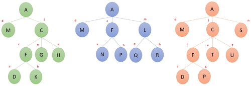
Figure 2. Unified BOM.

The last two edge categories (n-XOR and MUTEX) merely reflect the exclusive relationships across multiple nodes and edges (any edge containing more than two entities is eventually a hyperedge; however, for simplicity, we represent them as edges). The former indicates an exclusive-OR relationship between a set of children sharing the same parent, i.e., the edges connecting a parent with its children. An example of this is the relation between C and L, which appear as descendants of A at different BOM variants. The presence of A thus indicates that only one of C and L can be its child. We depict this relation by drawing a firm angle between edges AC and AL. If the XOR relation is between three or more edges, then the angle would stretch up to the two outermost edges. One might also encounter a situation where n out m children have to be chosen. Such conditions are represented by attaching a cardinality (n) label to the angle (e.g., see the 2-XOR edge connecting four offsprings of C). Although the n-XOR edge allows mutual exclusivity between nodes, it mandates the presence of at least one (or more) child node(s) (given the presence of the parent). In contrast, the MUTEX edge does not enforce this additional constraint; it simply indicates their mutual exclusivity. Let us consider the case of L and S for demonstration. Both of them are offsprings of A, but they do not appear together in any of the variant BOMs. Relating them through an XOR edge compels the presence of exactly one node in any BOM. However, this will disallow the representation of variant 1, which contains neither of them. We thus choose to connect the two nodes via a MUTEX edge. Formation of MUTEX and n-XOR edges are determined by the structural variations across individual BOMs, and the purpose (P_i) of their nodes. The latter indicates the function of an individual part in the manufacturing process. Parts with similar purpose in different BOMs are likely to be interchangeable. For example, in each BOM variant, F consists of two children with purpose a and b. Since both D and N are labeled with purpose a, they act as substitute to each other. Similarly, the children of C (except F) are labeled with the same purpose e and any two of them can be chosen for production. Finally, to account for the positional variation of nodes in different BOM variants (e.g., F in BOM 1 and 2), we follow the procedure prescribed in Romanowski and Rakesh Nagi (2004), i.e., choose the positioning at the lowest level.

3.1.2. Mapping of the UBOM to the supply chain

The unified BOM provides an exhaustive list of the parts that may be used to manufacture the illicit product. This list serves as the basis for categorizing the suppliers into different groups. Each group represents the set of suppliers for a specific ingredient; some may include multiple materials which are interchangeable. A functional supply network, however, will not include all categories at the same time. That decision depends on the product variant being manufactured and the strategy for sourcing its associated raw materials.

As an example, let us assume that illicit traders are interested in peddling the first variant of product A. The BOMs (Figure 1) associated with it indicates two inputs in the manufacturing process: M and C. The first item is a base part and can only be acquired through direct purchase. As for the second ingredient, the manufacturer has options for either direct purchase or in-house manufacturing. Pursuing the second option will again require additional procurement (F, G, and H) and/or additional manufacturing (F from D and N) operations. It is essential to reflect such variations in the supply network.

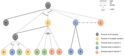
We accomplish this by transforming the original illicit network into another logical graph, $G^T=(V^T,E^T,E^C,A^T)$ (Figure 3). The number of stages in the new network remains unchanged (supplier, manufacturer, and consumer). However, additional nodes are incorporated into the supplier stage. The total number of nodes in the graph is upper bounded by the node-set cardinality in the UBOM, (B^U): $\left|V^T\right|\le \left|L^U\right|+2\left|I^U\right|+2.$ Here, we consider two nodes for each intermediary part (I^U) in the UBOM, indicating direct purchase (shaded gray) and in-house manufacturing (shaded orange), respectively. In the latter case, the manufacturer itself acts as the supplier of the specified product. Since the leaves (L^U) are direct-purchased parts and cannot be manufactured, only one supplier is considered for them. The remaining two nodes correspond to the manufacturer and consumer. The upper bound calculation is based on the assumption that all nodes are placed at a unique level/depth in the UBOM; any violation to this may lead to a bound increase. Each node is assigned a set of attributes A^T (e.g., material type and quality, production quantity, operational discreetness) for specification purpose. To illustrate the order of their selection, we further classify the supplier nodes into multiple tiers/echelons. Each tier corresponds to a particular level of depth in the UBOM (B^U); if a material is placed at depth n in the UBOM, its suppliers shall belong to tier n in the supply network. Tier 1 suppliers provide parts that are direct inputs to the manufacturing process. Tier 2(3) suppliers, on the other hand, provide parts that go into manufacturing of those inputs (parts provided by tier 1(2) supplier). If the selected Tier 1 suppliers are external firms, then there would be no need for tier 2 suppliers. However, if there exists a in-house manufacturing node in tier 1, then it will have to procure-dependent items from suppliers in tier 2. In other words, a tier n supplier will be included in the supply network only if n = 1 or if it supplies parts to a tier n – 1 in-house manufacturer. Thus, the manufacturer shall traverse through the supplier tiers in ascending order until all the suppliers in a tier turn out as seller nodes.

Figure 3. Base supply network corresponding to the UBOM.

To illustrate the diverse flows across supply network, we use multiple (AND, OR, MUTEX, and n-XOR) edge categories. Some of these (mostly AND/OR) connect nodes across different (successive) stages/echelons and represent possible transactions between corresponding entities. We thus call these physical edges E^P (marked green). Others (MUTEX/n-XOR/AND) represent the constraints associated with selection of a set of suppliers. We term them as constraint edges (E^C) and mark them red. Similar to the nodeset, the edgeset in G^T is also highly influenced by the UBOM. In fact, for each edge $e\in E^U$ in the UBOM, there should be a corresponding edge connecting their associated nodes in G^T (however, supplier (purchase) nodes are not allowed any connection with the preceding echelons). In addition, MUTEX edges connect the two variant (purchase and manufacturing) supplier nodes at each tier. With this, the construction of the base network is complete. In the following subsection, we describe our next task: the identification of interface points.

3.2. Searching for interface points in the licit supply network

The base network constructed in the previous subsection characterizes the entities capable of being suppliers in the illicit supply chain, but does not reveal their identity. To achieve this, we rely on another assumption: some of the raw materials are legally tradable and can be sourced from legal organizations (even if this is a controlled substance). Thus, we search the legal supply network to identify all potential supplier nodes, i.e., the interface points. Mathematically, one can relate this to a variant of the subgraph isomorphism problem: Minimal Candidate Sets Problem (MCSP), see Moorman et al. (2018). Here, we consider the illicit network $G^T=(N^T,E^T,A^T)$ as the template and licit network, $G^D=(V^D,E^D,A^D)$ as the world or data graph. For each $v\in N^T,$ we want to find $\underset{f\in \mathcal{F}(G^T,G^D)}{\cup }f(v),$ where $\mathcal{F}(G^T,G^D)$ denotes matches between the template and the world graph. Unlike assignment problems, we do not require one-to-one matching between the nodes, i.e., the same node in the data (template) graph can be matched to two different template (data) nodes. Thus, solving the problem will require enumerating the similarity score between nodes of the two sets. This in turn depends on similarity scores for individual attributes (e.g., traded component, corruptibility, operational discreetness). Depending on the product and context, compatibility in some attribute(s) may be mandatory (e.g., for an organization to be an illicit supplier, it must trade in a product that is involved in the manufacturing of the illicit product). We use this information to accelerate the matching process by deploying a two-step procedure discussed in Date (2018). The first step here is filtering, where we check if a pair consisting of template node $i\in V^T$ and data node $j\in V^D$ is sufficiently compatible in terms of critical attributes. If not, we directly set the similarity score s_ij = 0. Otherwise, we proceed towards computing their similarity as a weighted function of their attribute similarities: $s_{ij}=\sum _k{w}_k{s}_{ij}^k.$ Here, $s_{ij}^k$ denotes the similarity of attribute k between node i and node j. The scoring mechanism may vary across different attributes. Thus, they are normalized to a range from zero to one. To facilitate customization, we offer two user-defined parameters: the weights of different attributes (${\left\{w_k\right\}}_{k=1}^K$), and the threshold similarity score (ϵ). With these, we can formally define the interface points as follows: $${\mathcal{I}}_p=\{q\in V^D:s_{pq}>ϵ\}\forall p\in V^T.$$ In other words, ${\mathcal{I}}_p$ indicates the set of nodes in the licit network that sufficiently match the characteristics of supplier p in the illicit network. Our next step is to integrate these nodes into the illicit network.

3.3. Augmentation of base network

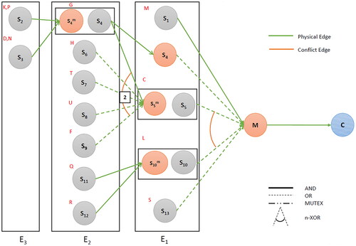
In this step, we augment the base supply network (G^T) into a broader network $G^I=(V^I,E_P^I,E_C^I,W^I,C^I).$ This involves replacing each direct-purchase supplier node p in the base network by its matched set of interface points ${\mathcal{I}}_p,$ as seen in Figure 4. For those without any matching, we can consider a set of nodes indicating possible facility locations/regions. The same approach is applicable to other stages, unless otherwise specified. We also modify the edge-set to define the relationships between these new nodes. Each edge in the base network (G^T) represents a connection between two (or more) specific categories of supply network entities (e.g., manufacturer, supplier of specific part, consumer). The augmented graph consists of multiple entities under each category. It is thus logical to replace each original edge in G^T by a set of edges that connect all pairs of nodes belonging to the Cartesian Product of the two categories (incident in the original edge). For example, only edge exists between category M and C in G^T. However, in the augmented graph, M and C have multiple representations: $M=\{M_1,M_2,M_3\},C=\{C_1,C_2\}.$ Thus, there should be an edge corresponding to every element in the following set: $$M\times C=\{(M_1,C_1),(M_1,C_2),(M_2,C_1),(M_2,C_2),(M_3,C_1),(M_3,C_2)\}.$$

Figure 4. Augmented graph.

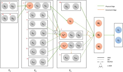
For visual clarity, we only show the edges between the groups. We additionally note the exclusion of edges between supplier nodes (explained in Section 3.1.2); edges between two manufacturing nodes or supplier and manufacturing nodes are allowed. Let us now discuss the node and edge weights, which would serve as basis for our optimization model. The former refers to the price/risk involved in manufacturing or purchasing a part, whereas the later is associated with its logistics. We assign weights only to physical edges, since they alone form the supply network; constraint edges serve as side constraints and restrictions. During weight calculation, a variety of factors need to be taken into account, (e.g., price and quality for node weights; physical distance and interception probability for edge weights). These are represented by q (nodes) and r (edges). Similarity score of the incident nodes (s_ij) is another crucial factor, since it measures their possibility of actually participating in an illicit supply chain. Acknowledging all these issues, we represent the weights as follows: $$w_u=\frac{f(q_u^1,\dots ,q_u^n)}{s_{ui}}\forall u\in {\mathcal{I}}_i{c}_{uv}=\frac{f(r_{uv}^1,\dots ,r_{uv}^m)}{\frac{1}{2}(s_{ui}+s_{vj})}, \forall u\in {\mathcal{I}}_i,v\in {\mathcal{I}}_j.$$

4. Extracting dissimilar supply network topologies

The graph constructed in the preceding section is a generalized representation of the illicit supply network, containing all entities suspected of participating in it. The actual (illicit) supply network should therefore be its subgraph. Our goal in this section is to specify the topology of this network, i.e., predict the entities forming the supply chain and their possible relationships. Unlike traditional approaches, we avoid declaring a single network configuration as the most likely one. Instead, we look for a set of networks that are efficient and “sufficiently dissimilar” (formally defined in Section 4.3). The rationale for our decision is that illicit supply chains are not formed purely around the objective of cost/logistical efficiency. This justifies the prudence in tracking multiple networks. However, an analyst or law enforcement investigator might not benefit from seeing numerous supply chain networks that differ simply by one supplier. They would rather examine a variety of networks that cover the space of “likely” possibilities. Our problem formulation allows users to enjoy this amenity in a flexible manner. The following subsections discuss the problem setting in detail along with an integer linear programming formulation for its representation.

4.1. Problem definition

In this problem setting, we have the illicit supply network represented as a directed acyclic graph, $G_I=(V,E^P,E^C,c,w).$ Each node in V represents an entity suspected of involvement as a supplier, manufacturer, or consumer in the illicit supply chain; $w:V\to R_{+}$ represent their weights. The suppliers are again classified into multiple tiers (e.g., three in Figure 4). Generalizing, we can simply consider the nodeset comprising q groups of supply network entities, i.e., $V={\cup }_{i=1}^q{\lambda }_i.$ We denote Λ as the set of these groups. A viable network (tree) can contain at most one node from a particular group; however, only a set of groups, ${\Lambda }_R\subseteq \Lambda$ are required to be present in it. Whether entities from other groups are present or not is unknown. The supply network is eventually formed with physical edges (E^P) and their cost ($c:E^P\to R_{+}$). Additional constraints (see Section 4.2) are derived from the constraint edges by converting them into distinct sets: R_A, R_M, and $R_{\ell X}.$ With these information available, our goal is to search the graph for p-dissimilar (i.e., the p-best structures that are mutually dissimilar by some minimum quantity) supply network structures, which in our case forms a tree. The following subsections discuss the mathematical formulation of this problem.

4.2. Mathematical formulation for minimum-cost tree

We begin with an integer linear programming formulation for finding a single, minimum cost tree (this will later be extended to p-dissimilar trees in Section 4.3). Although we recognize that this can be found by an algorithmic procedure similar to cost roll-up (see also Algorithm 1), the optimization model is needed for finding the p-best trees, as we will see later in Section 5.2. Furthermore, it might also be easier for the analyst to use a standard optimization solver. While searching for the optimal solution, we are faced with three questions: (i) whether an edge (transaction) is in the optimal tree (network), (ii) whether a node (entity) is in the optimal tree (network), and (iii) whether any node from a group participates in the optimal tree. These questions eventually define our three decision variables. Before defining the decision variables and mathematical formulation, we present the notation used.

First, we use Λ to denote the set of groups we have, with ${\Lambda }_r\subseteq \Lambda$ refering to the groups that are required. Each group, denoted by ${\lambda }_i\in \Lambda ,$ includes entities defined as λ_ij. We use E^P to refer to physical edges, $E_A^P$ to physical AND edges, $E_O^P$ to physical OR edges. All edges are assigned a cost c_e; this can represent a notion of cost, “detectability”, or other discriminating measures. Let $\Gamma ({\lambda }_{gi})$ be the set of edges incident to λ_gi. $\mathcal{R}=R_A\cup R_M\cup R_{\ell X}$ includes the relationship rules between the selected groups. Specifically, R_A, R_m, and $R_{\ell X}$ indicate the set of AND, Mutual exclusive and $\ell$-XOR relationships (for $\ell \ge 1$), respectively. For the $\ell$-XOR relationships, we also define L_r as the number of nodes required in $\ell$-XOR relationship $r\in R_{\ell X}.$ With the notation defined, we may proceed with our decision variables.

We define three binary decision variables: x_e is 1 if edge $e\in E^P$ is present in the optimal tree and 0 otherwise; z_g = 1 if group $g\in \Lambda$ is present in the optimal tree; and y_gi = 1 if node ${\lambda }_{gi}\in V$ is present in the optimal tree. We also note that y_gi can be treated as continuous because it will automatically take on binary values. Finally, we are ready to present the mathematical formulation as in (1)(1) $$\min \sum _{e\in E^p}{c}_e{x}_e+\sum _{{\lambda }_{gi}\in V}{w}_{gi}{y}_{gi}$$(1) –(11)(11) $$z_g\in \{0,1\},\forall g\in \Lambda .$$(11) : (1) $$\min \sum _{e\in E^p}{c}_e{x}_e+\sum _{{\lambda }_{gi}\in V}{w}_{gi}{y}_{gi}$$(1) (2) $$\mathrm{s}.\mathrm{t}. \sum _{i\in {\lambda }_g}{y}_{\mathit{\text{gi}}}{=z}_g,\forall g\in \Lambda ,$$(2) (3) $$z_g=1,\forall g\in {\Lambda }_r,$$(3) (4) $$y_{gi}\ge x_e,\forall {\lambda }_{gi}\in V,e\in \Gamma ({\lambda }_{gi}),$$(4) (5) $$\sum _{e\in E}{x}_e=\sum _{{\lambda }_{gi}\in V}{y}_{gi}-1,$$(5) (6) $$z_i+z_j\le 1,\forall ({\lambda }_i,{\lambda }_j)\subseteq r,\forall r\in R_M,$$(6) (7) $$\sum _{k\in {\mathcal{C}}_r}{z}_k=L_r,\forall r\in R_{\ell X},$$(7) (8) $$z_i=z_j,\forall \left({\lambda }_i,{\lambda }_j\right)\subseteq r,\forall r\in R_A,$$(8) (9) $$x_e\in \{0,1\},\forall e\in E,$$(9) (10) $$y_{gi}\in \{0,1\},\forall i\in {\lambda }_g,g\in \Lambda ,$$(10) (11) $$z_g\in \{0,1\},\forall g\in \Lambda .$$(11) In the objective function (1)(1) $$\min \sum _{e\in E^p}{c}_e{x}_e+\sum _{{\lambda }_{gi}\in V}{w}_{gi}{y}_{gi}$$(1) , we minimize the total weight/cost of the nodes and edges that are selected. Constraints (2)(2) $$\mathrm{s}.\mathrm{t}. \sum _{i\in {\lambda }_g}{y}_{\mathit{\text{gi}}}{=z}_g,\forall g\in \Lambda ,$$(2) restrict only one node from each selected cluster to be present in the tree. The second set of constraints in (3)(3) $$z_g=1,\forall g\in {\Lambda }_r,$$(3) enforce that certain groups are required to be present in the tree. Constraints (4)(4) $$y_{gi}\ge x_e,\forall {\lambda }_{gi}\in V,e\in \Gamma ({\lambda }_{gi}),$$(4) impose that a node can be selected if at least one of each adjacent edges is in the tree. Then, (5)(5) $$\sum _{e\in E}{x}_e=\sum _{{\lambda }_{gi}\in V}{y}_{gi}-1,$$(5) states that the structure obtained needs to form a tree. Although typically this constraint by itself is not enough, in our case the underlying graph is a directed acyclic graph (see Section 4.1), and hence, the traditional cycle elimination constraint is not necessary. The next three families of constraints in (6)(6) $$z_i+z_j\le 1,\forall ({\lambda }_i,{\lambda }_j)\subseteq r,\forall r\in R_M,$$(6) , (7)(7) $$\sum _{k\in {\mathcal{C}}_r}{z}_k=L_r,\forall r\in R_{\ell X},$$(7) , (8)(8) $$z_i=z_j,\forall \left({\lambda }_i,{\lambda }_j\right)\subseteq r,\forall r\in R_A,$$(8) are derived from the constraint edges (AND, MUTEX, and n-XOR, respectively). Finally, constraints (9)(9) $$x_e\in \{0,1\},\forall e\in E,$$(9) –(11)(11) $$z_g\in \{0,1\},\forall g\in \Lambda .$$(11) are our binary variable restrictions.

4.3. Formulation for p-dissimilar trees

The previous section discussed the formulation for identifying the minimum weight/cost tree. In this section, we want to extend it to p-dissimilar trees for diversification purposes of law enforcement. Before that, we need to define the notion of dissimilarity. Based on the formulation described in Erkut and Verter (1998), we represent the dissimilarity between two trees a and b as: $$D(a,b)=1-S(a,b), \mathrm{ }\text{where},\mathrm{ } S(a,b)=\frac{1}{2}\left(\frac{L\left(a\cap b\right)}{L\left(a\right)}+\frac{L\left(a\cap b\right)}{L\left(b\right)}\right).$$

Here, S(a, b) indicates the similarity between the two trees, whereas $L(.)$ indicates the number of elements (node/edge) in a tree. We can use either of these to define the dissimilarity requirement. Any set of feasible trees (satisfies constraints (2)(2) $$\mathrm{s}.\mathrm{t}. \sum _{i\in {\lambda }_g}{y}_{\mathit{\text{gi}}}{=z}_g,\forall g\in \Lambda ,$$(2) -(11)(11) $$z_g\in \{0,1\},\forall g\in \Lambda .$$(11) ) that meets this requirement while accumulating the least cost is considered as optimal. We again provide the formulation after describing the notation and defining our decision variable.

Let $\mathcal{T}$ be the set of feasible trees. Each tree is associated with a cost ${\sigma }_i,i\in \mathcal{T};$ D(i, j) represents the dissimilarity between trees $i,j\in \mathcal{T}.$ Finally, two important parameters are δ and p. δ is the minimum dissimilarity required between any two trees present in the optimal solution. p serves as a budget in the form of the number of dissimilar trees obtained. This leads to a new binary decision variable in the form of: u_t = 1, if and only if if tree $t\in \mathcal{T}$ is present in the optimal set. Finally, the mathematical formulation is shown in (12)(12) $$\min \sum _{t\in \mathcal{T}}{\sigma }_t{u}_t$$(12) –(15)(15) $$u_t=\{0,1\}\forall t\in \mathcal{T}.$$(15) : (12) $$\min \sum _{t\in \mathcal{T}}{\sigma }_t{u}_t$$(12) (13) $$u_i+u_j\le 1,\forall i,j\in \mathcal{T}:D(i,j)<\delta ,$$(13) (14) $$\sum _{t\in \mathcal{T}}{u}_t=p$$(14) (15) $$u_t=\{0,1\}\forall t\in \mathcal{T}.$$(15)

The objective (12)(12) $$\min \sum _{t\in \mathcal{T}}{\sigma }_t{u}_t$$(12) here is to minimize total cost from the selected trees. Equation (13)(13) $$u_i+u_j\le 1,\forall i,j\in \mathcal{T}:D(i,j)<\delta ,$$(13) states the dissimilarity constraints over optimal trees, whereas (14)(14) $$\sum _{t\in \mathcal{T}}{u}_t=p$$(14) indicates the number of required trees. Finally, (15)(15) $$u_t=\{0,1\}\forall t\in \mathcal{T}.$$(15) refers to the binary nature of the decision variable.

A potential drawback of this formulation is the requirement of all feasible trees, even when the value of p is small. An alternative approach would involve sequential generation of the dissimilar trees, which may reach the solution going through a smaller number of trees. This can be done by adopting an algorithmic solution approach, discussed next.

5. Graph-theoretic approach

5.1. Relationship to family of STPs

We begin this section with a discussion on the nature of our problem as stated in Section 4. The purpose is to discover possible connections between our problem setting and existing problem genres, which can provide guidance on its solution approach. In the context of graph theory, the GSTP is perhaps the closest representation of our problem. Taking a graph with multiple node groups as input, the optimal solution to the GSTP is a minimum-cost tree that includes at least one node from each group. Our problem can be adopted to most of these features (requirement of exactly one node per group is a feature of Group Spanning Tree problem, a variant of GSTP). However, the key difference between the two problems lies in the number of groups to be spanned in the optimal tree. Whereas the GSTP requires all groups to be spanned, our problem requires the spanning of only a subset (${\Lambda }_r\subseteq \Lambda$) of these groups. The decision to include other groups is guided by a set of constraints provided as input in constraint set R. Selection of the spanning groups resembles the STP, since we have a set of Terminal groups (spanning required), and a set of Steiner groups (spanning optional). Once the groups are identified, the problem reduces to a GSTP. In other words, our problem can be thought of as a generalization of the GSTP, where the groups to be spanned are unknown and constrained by a set of relationships. This invokes the concept of a new variant of STP: we refer to it as the Generalized Group Steiner Tree Problem (GGSTP). Its formal definition is given in Definition 1.

Problem Definition 1 (GGSTP):

Instance: An undirected graph $G=(V,E)$ with non-negative edge-cost $\{c_e:e\in E\}$, a set of Terminal vertex groups $\{T_1,\dots ,T_m\}$, a set of Steiner vertex groups $\{S_1,\dots ,S_n\}$, and a set of relationships $\mathcal{R}$ between groups.

Solution: A minimum-cost tree T of G that spans at least one node from each Terminal group and satisfies all relationships in $\mathcal{R}.$

Objective: Minimize the sum of edges in the tree.

Theorem 1.

The GGSTP is NP-hard.

Proof.

Consider an instance of GGSTP with all groups are terminal vertex groups (i.e., ${\cup }_{i=1}^m{T}_i=V$) with no Steiner vertex groups. Further, let $\mathcal{R}=\varnothing .$ Then, this is the GSTP problem, which is NP-hard (Ihler, 1991). Hence, the GGSTP is at least as hard as GSTP. □

The definition provided is more general and aims to introduce this interesting problem. In our specific application on illicit trade, there are some important differences; for example, our graph is a directed acyclic graph, which simplifies the situation. We also impose that the optimal tree can contain at most one node from each selected group (both Terminal and Steiner). Finally, we aim to derive a series of p diverse solutions/trees. All these changes are incorporated in our algorithm design, described in the next subsection.

5.2. Approach to identify dissimilar trees

The core objective of our algorithm is to identify the set of p-best trees with at least δ amount of mutual dissimilarity, $\mathcal{P}(p,\delta ).$ Here, $p\ge 1,$ and $0\le \delta \le 1.$ As mentioned earlier, solving this as an optimization problem requires prior knowledge of all feasible trees. Another option is to identify the k-most efficient trees and then search for p-dissimilar trees among them in ascending order (k > p). This again can be formulated as an optimization problem; but we do not know what the value of k should be to find $\mathcal{P}.$ Setting the value of k too high may increase computational cost while setting it too low will fail to capture the desired number of trees. Considering this dilemma, we design our algorithm to sequentially generate trees in increasing order of cost until p of these are retained. This is done in three major steps: (i) identification of the minimum cost tree; (ii) inclusion of additional trees; and (iii) extraction of dissimilar trees. The following subsections discuss them in detail.

5.2.1. Identification of minimum-cost tree

The first step in our algorithm involves identifying the least-cost tree (with specified attributes) within the given graph. A key issue here is the presence of both types of supplier nodes (In-House Manufacturing (IHM) and Direct-Purchase (DP)) in the same group; only one of them can be selected. Since DP nodes are leaves, their inclusion (in the tree) only incurs the costs (node and edge weights) associated with the part they supply. On the other hand, selection of IHM nodes requires consideration of both manufacturing and raw-material sourcing costs, which are harder to estimate directly (as discussed in Section 3.1.2). We thus need to fully characterize the cost and choices for IHM nodes. For this, we adopt an approach similar to the cost roll-up process in an Enterprise Resource Planning (ERP) system by starting with the deepest echelons and moving towards the final product (or customer). As seen in Section 3, our supply network consists of multiple echelons $\mathcal{E}=\{E_1,\dots ,E_Z$}. For ease of computation, we consider an additional echelon E₀ with a single node d that has connections from all customer nodes. The weights of this node and its incident edges is zero. The deepest level Z cannot have any IHM node by definition, thus we start with $E_{Z-1}.$ To determine the cheapest cost of including a specific IHM node $v\in E_{Z-1},$ we need to find the minimum cost in-tree rooted at v. This involves finding the cheapest node corresponding to each required and optional group, i.e., the node u with least value of $w_u+c_{uv}.$ Using the relationship set $\mathcal{R}$ for v, we can then form the least cost sub-tree. Once the (cheapest) cost of all IHM nodes in Echelon $E_{Z-1}$ are computed, we can move to $E_{Z-2}$ and repeat the same process. The same technique will be applied at other echelons as we move up the supply chain. However, for non-supplier echelons, we find the cheapest cost of inclusion (and corresponding substructure) at all nodes. Prior to termination, our algorithm removes the dummy node from the optimal tree. Our approach is demonstrated through a pseudo-code (Algorithm 1). Two key functions involved here are the CheapestEdge (finds the cheapest node from every source group of an IHM node) and Compose (constructs the minimum cost substructure with respect to the available constraint set $\mathcal{R}$ (Compose function).

Algorithm 1.

Identifying Minimum Cost Tree

1: function Get Mincost Tree($G=(V,E^P,c,w),\mathcal{E},\mathcal{R}$)

2:  $i\leftarrow Z-1$                     // Starts at echelon $E_{Z-1}$

3:  while $i\ge 0$ do

4:   $M_i\leftarrow \mathit{Characterize}(G,i)$    // Find set of IHM nodes in echelon E_i

5:   for all $m\in M_i$ do

6:    $B(m)\leftarrow \varnothing$    // Creates Tree corresponding to an IHM node m

7:    $P(m)\leftarrow \mathit{Source}(G,m)$    // Finds the set of suppliers in echelon i – 1

8:    ${\sigma }_m\leftarrow 0$    // Assigns cost to the tree rooted at m

9:    for all $j\in P(m)$ do

10:     $e_j\leftarrow \mathit{CheapestEdge}(j,m,{\sigma }_m)$    // Finds the cheapest edge between group j and node m

11:    end for

12:    (${\sigma }_m,B(m))\leftarrow \mathit{Compose}(\underset{j}{\cup }{e}_j,\mathcal{R})$    // Using the relationship $\mathcal{R},$ we aggregate the cost

13:                     //      and the sources of m

14:   end for

15:   $i\leftarrow i-1$

16:  end while

17:  $K_1\leftarrow B(m)\setminus d$    // Removes dummy node $d\in$ E₀ from optimal tree

18:  return K₁

19: end function

5.2.2. Inclusion of additional trees

With knowledge of the best (least cost) tree available, we proceed to the second step of our algorithm: identifying the set of next best trees. We represent them by the set $\mathcal{K}=\{K_1,\dots ,K_n\},$ where ${\sigma }_{K_i}\le {\sigma }_{K_{i+1}}.$ For its implementation, we follow a Murty-like enumeration approach (see Murty (1968)) that disallows the best solution (by adding an appropriate constraint) to enumerate the next best solution iteratively until the k best supply networks are obtained. In essence, this involves deriving new mutually exclusive sets of constraints (let us assume it to be $\mathcal{C}$) from the prior minimum-cost tree structure and including them separately to the minimum-cost tree problem. Thus, we shall have $\left|\mathcal{C}\right|$ variants of the minimum-cost tree problem. Solving them results in a set of candidate trees, $A_j=\{A_{j1},\dots ,A_{j\left|\mathcal{C}\right|}\};$ we can use Step 1 as a subroutine here. Among these, the tree with the least cost is considered as the next best tree, i.e., $K_j=\arg {\min }_{A_{jl}}\left\{{\sigma }_{A_{jl}}\right\}.$ For brevity, we do not provide detailed explanation of our approach and refer readers to Murty (1968). However, we do provide a sample example to demonstrate the generation of the constraints. Let us assume $K_1=\{e_1,e_2,e_3\}$ to be the minimum-cost tree in the graph. To derive the second best cost tree (K₂), we shall need to define the following constraint sets: $${\mathcal{C}}_{11}=\left\{\overline{e_1}\right\},{\mathcal{C}}_{12}=\{e_1,\overline{e_2}\},{\mathcal{C}}_{13}=\{e_1,e_2,\overline{e_3}\}.$$

Here, the first constraint indicates that the optimal tree shall not consist of edge e₁ (presence of overhead dash). The second constraint mandates the presence of e₁ and absence of e₂ in the optimal tree. Similarly, the third constraint requires the presence of e₁ and e₂ in the optimal solution while prohibiting e₃. Construction of these constraints allow consideration of the whole solution space except K₁. Next, we consider three problem settings corresponding to the addition of each new constraint set. Solving them eventually provides us with three trees, the minimum of which is K₂ (the next least-cost solution). The remaining trees are preserved for future computation. In a similar approach, we derive new constraints with respect to K₂ and obtain a new set of trees as well. The third best tree is the one with the minimum cost among the new trees and the remaining trees from the previous iteration. Once $\left|\mathcal{K}\right|$ reaches a certain number, we can move to the final step.

Algorithm 2.

Identifying k-best Trees

1: function Get k Tree($K_1;k;G=(V,E^P,c,w),\mathcal{E};R$)

2:  $\mathcal{K}\leftarrow \left\{K_1\right\}$    // Initialize the best tree set with the least cost tree

3:  $i\leftarrow 2$     // Start calculation for second tree

4:  $A\leftarrow \varnothing$    // Set of all unselected trees

5:  while $\left|\mathcal{K}\right|<k$ do

6:   $C_{i-1}\leftarrow \mathit{Murty}(K_{i-1})$  // Collection of constraint sets for the previous tree

7:   for all $j\in {\mathcal{C}}_{i-1}$ do

8:    ${\mathcal{R}}_j\leftarrow R\cup \left\{j\right\}$   // Add individual constraint sets to the usual constraint

9:    $A_j\leftarrow \mathrm{GET}\mathrm{MIN}\mathrm{COST}\mathrm{TREE}G=(V,E^P,c,w);\mathcal{E};R_j$

10:    $A\leftarrow A\cup A_j$

11:   end for

12:   $K_i\leftarrow \arg {\min }_{A_j}{\sigma }_{A_j}$

13:   $A\leftarrow A\setminus \left\{K_i\right\}$

14:   $\mathcal{K}\leftarrow \mathcal{K}\cup \left\{K_i\right\}$

15:   $i\leftarrow i+1$

16:  end while

17:  return $\mathcal{K}$

18: end function

5.2.3. Extraction of dissimilar trees

Our third and final step involves filtering the trees in $\mathcal{K}$ to identify $\mathcal{P}=\{P_1,\dots ,P_p\},$ the set of p-best dissimilar trees. It seems reasonable to start with the minimum-cost tree as the first member of $\mathcal{P}.$ Since trees in $\mathcal{K}$ are ordered based on their weights, the next member of $\mathcal{P}$ should thus be the first tree differing from P₁ by at least δ. And the third member should be the first tree differing from both the members of P by at least δ. Thus the search for pth member in $\mathcal{P}$ can be represented as: $$P_p=K_m:m=\underset{j}{\arg \min }\{K_j:D(K_j,P_l)\le \delta \}; \forall l=1,\dots ,p-1.$$

Algorithm 3.

Identifying p-best dissimilar Trees

1: function Get Dissimilar Tree($\mathcal{K},p,\delta$)

2:  $\mathcal{P}\leftarrow \left\{K_1\right\}$    // Minimum cost tree is in the dissimilar set

3:  $i\leftarrow 2$      // Comparison will start from second best tree

4:  while $\left|\mathcal{P}\right|<p$ do

5:   ${\mathcal{D}}_i\leftarrow \varnothing$    // Set for storing dissimilarity scores

6:   for all $m\in \mathcal{P}$ do

7:    ${\mathcal{D}}_{im}=\mathcal{D}(K_i,m)$   // Calculation of dissimilarity

8:    ${\mathcal{D}}_i\leftarrow {\mathcal{D}}_i\cup \left\{{\mathcal{D}}_{im}\right\}$

9:   end for

10:   if $\mathit{min}{\mathcal{D}}_i\le \delta$ then  // Checks if the minimum value in the set less than δ

11:    $\mathcal{P}\leftarrow \mathcal{P}\cup \left\{K_i\right\}$

12:   end if

13:   $i\leftarrow i+1$

14:  end while

15:  return $\mathcal{P}$

16: end function

We can execute Algorithms 2 and 3 sequentially or alternately. The first approach will generate a large number of trees in step 2 before proceeding to step 3. The latter will create a fixed number of trees before step 3. If that fixed number is p, then the algorithm will take at most $2p-1$ additional trees to construct the dissimilar set.

We could also adopt another distinct approach to this problem. Since our objective is to find p distinct trees that are δ dissimilar from each other, it is natural to think of the problem in terms of cliques. Consider that we develop a graph $G^D=(N^{\mathcal{K}},A^D),$ where $N^{\mathcal{K}}$ represent the set of nodes corresponding to the k-best trees, $\mathcal{K},$ and A^D is a set of edges where an edge exists between a pair of node $i,j\in \mathcal{K}$ iff $D(i,j)\ge \delta .$ One could find the maximum clique that includes the first node, repeat this for a few other nodes that were not present in this clique, or find the maximal cliques from each node in $N^{\mathcal{K}}.$ If this approach results in one or more cliques that are of size p or greater, we can pass them on to the analyst for further investigation. If the cliques are not adequate (for law enforcement purposes), one can expand the search on the k-best trees and repeat the process. The complexity of forming the graph G^D is $O(k^2).$ The well-known Bron–Kerbosch (or similar) algorithm can be applied to find the maximum clique. As δ increases and G^D becomes sparser, we can explore more specialized algorithms for sparser graphs (see, e.g., Buchanan et al. (2014)).

6. Illustrative case study

Our discussion up to this point has primarily been on the context and functioning of our proposed methodology. In this section, we shift our attention to its implementation in practical settings as well as the interpretation of the results obtained. For this purpose, we present a semi-real case study on the counterfeit footwear trade, which makes up a significant (22% by seized value (OECD and European Union Intellectual Property Office, 2019)) share of the illicit (counterfeit) trade volume. The following paragraph discusses issues pertinent to the construction of this case study as well as its use in the formation of the generalized supply network.

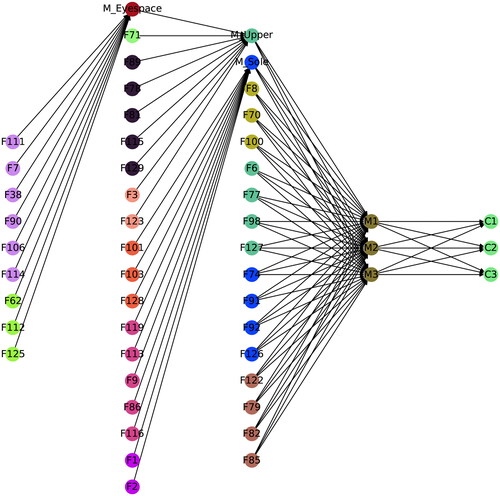
We first construct the UBOM for a counterfeit shoe as seen in Figure 5. This merges three three major shoe variants: laced shoe, slip-on shoe, and sandals. Information on the individual BOM is available online, although the detail may vary across sources. Figure 6 shows the corresponding base supply network with three supplier echelons. We can also see three IHM nodes here (marked yellow): M_Eyespace, M_Upper, and M_Sole. Figure 7, on the other hand, represents the aggregated licit supply network for the items in the UBOM. Its construction required the name and location of organizations involved in the trade of specific parts, as well as their roles (exporter or importer) in it. We used the open search tool in Panjiva (S & P Global Market Intelligence, 2022) to retrieve these; however, organizational attribute data (e.g., product pricing, logistic cost, transparency) were unavailable. We thus assumed a generic likelihood for this nodes of participation in illicit trades. For exporter nodes, this corresponded to the illicit trade environment index score by the Economist Intelligence Unit (Economist Intelligence Unit, 2018); for the importer nodes, this was based on crime rate of the facility locations (World Population Review, 2022). Both scores were normalized between zero and one. A threshold score of $ϵ=0.7$ was set to identify the interface points, which are marked red in the figure. Figure 8 shows the augmented graph, which comprises of 51 nodes and 88 edges. Here, nodes are color-coded to distinguish the groups to which they belong (compare with Figure 6). Node and edge weights are assigned by a random value generator. Unavailability of credible information for some attributes led us to anonymizing the company names (as F1, F2,…) so that we do not incorrectly implicate any of them being a member of the illicit supply chain. Finally, we run our algorithms on the augmented network with the parameter setting: p = 10, $\delta =0.6.$ For verifying the first two algorithms, we also solve the optimization model in Gurobi (Gurobi Optimization, 2022).

Figure 5. Unified BOM for footwear.

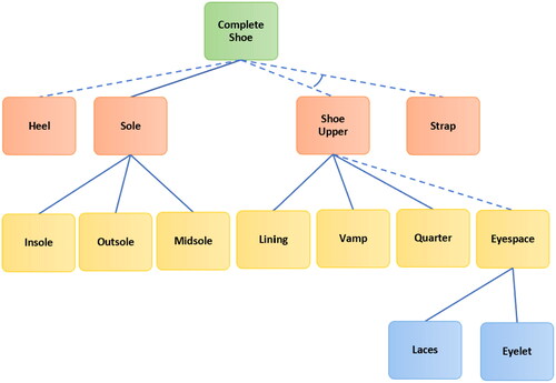
Figure 6. Base illicit supply network.

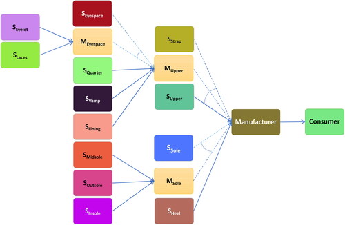
Figure 7. Licit supply network.

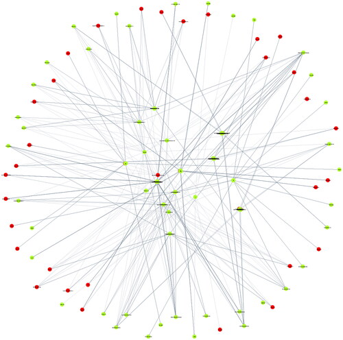
Figure 8. Augmented illicit supply network.

6.1. Result analysis

Following the completion of our experiment, we turn our focus to the result analysis, which is summarized in Tables 1 to 3. Table 1 displays the primary output, i.e., 10 best (cheapest) supply networks that are mutually dissimilar by 0.6 or more. The organizations and BOM variants that are most prevalent in these networks are highlighted in Table 1 and 3, respectively. Let us now discuss the practical insights these results offer on the illicit supply chains. From the simplest perspective, this approach provides us the knowledge of the 10 best dissimilar supply networks. In other words, they are the most likely candidates for the actual supply network. They may also be interpreted as alternative distribution pathways criminals can use if their existing network is disrupted; the extent of disruption is explained by δ. It is important to note that, by investigating these 10 networks sequentially or simultaneously, we can bring 47.06% of the nodes in the suspected networks under surveillance. This measure (cumulative percentage) may be of interest to some analysts, where he/she would like to identify the number of trees/networks to extract for reviewing a certain number/percentage of nodes. This will primarily depend on the value of p and δ. Another crucial insight here is the identification of vital entities, which appear frequently in the diverse networks. Thus, disrupting them results in simultaneous breakdown of multiple supply networks. None of the entities in our case (see Table 2) exhibit such prominence; mostly due to higher value of δ. However, they still inform one of the entities that are preferred at each stage.

Table 1. Analysis of results for Dissimilar Trees.

Rank	Entities Involved	Cumulative Coverage(%)
1	$C_1,M_1,F_{100},F_{74}$	7.84
2	$C_2,M_3,F_{70},F_{91}$	15.69
3	$C_2,M_3,F_{127},F_{91}$	19.61
4	$C_3,M_2,F_8,F_{74}$	23.53
5	$C_2,M_1,F_6,F_{126}$	27.45
6	$C_3,M_1,F_{91},F_{98}$	29.41
7	$C_1,M_3,F_{92},F_6$	31.37
8	$C_1,M_2,F_8,M_{\mathit{Sole}},F_1,F_{101},F_{119}$	39.22
9	$C_2,M_2,F_{92},F_{98}$	39.22
10	$C_2,M_3,F_{92},F_{123},M_{\mathit{Upper}},F_{129},F_{71}$	47.06

Table 2. Analysis of results for Vital Entities

Stage	Rank	Entity	Frequency
Supplier	1	F91 (Sole)	3
	2	F92 (Sole)	3
	3	F8 (Strap)	2
Manufacturer	1	M2	4
	2	M3	3
	3	M1	3
Consumer	1	C1	4
	2	C2	4
	3	C3	2

Table 3. Analysis of results for Preferred Design.

Design Variant	Frequency
Slip-on Shoe	6
Sandal	4

Finally, the resultant networks also hint at possible trends in the design and manufacturing of the illicit product. For example, none of the supply networks corresponded to the laced shoe variant design. Furthermore, most of the supply networks avoided IHM (except in 8 and 10). Such insights would help the analyst find the causes underlying these situations and take appropriate measures to design a more effective scheme for disrupting the illicit supply chain.

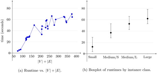
6.2. Runtime analysis

To show the scaling of our algorithm, we ran experiments on networks of different sizes. It was implemented in Python using Jupyter Notebook. The following Figure 9(a) shows our runtime for different values of $\left|V\right|+\left|E\right|;$ all reported results are average runtimes and their standard deviations out of 10 experiments for each setup (see Figure 9(b) for a visualization of minimum, average, and maximum runtimes for different graph sizes). It is important to note that our algorithms are designed to operate sequentially. Parallelization of specific operations and use of more efficient coding platform is expected to improve the run time.

Figure 9. The obtained computational runtimes for graphs of 28 different $\left|V\right|+\left|E\right|.$ All runtimes presented are averages of 10 experiments. Figure 9(b) shows the average, minimum, and runtimes for each family of graphs, separated as small ($\left|V\right|+\left|E\right|<130$), medium-small ($130\le \left|V\right|+\left|E\right|<210$), medium-large ($210\le \left|V\right|+\left|E\right|<280$), and large ($\left|V\right|+\left|E\right|\ge 280$).

7. Conclusions and future work

The first, and often the most difficult, step in countering illicit trades is to expose their clandestine supply chains. In this research, we present a quantitative approach that helps accomplish this goal using limited information. A number of novel concepts and methodologies are featured in the study, including the unification of alternate BOMs, their mapping onto supply networks, detection of interface points, search for dissimilar trees/supply networks and the discovery of the GGSTP. Furthermore, implementation of our methodology in the case study shows its applicability in real-life scenarios. We thus expect our research to benefit both academicians and professionals from relevant domains.

For future research endeavors, there remain several interesting opportunities. A natural extension of this research would be to relax some of the assumptions used in the problem formulation (e.g., single supplier sourcing, tree structure of supply network) and incorporate more realistic conditions (e.g., different transportation strategies, simultaneous deployment of BOM variants). There is also opportunity to adapt this problem into licit supply network design. In fact, diversification of legal supply chains has received significant attention in recent times (Savoy & Ramanujam, 2022). Besides this, the newly introduced the GGSTP remains an exciting open problem to solve efficiently or with bounded approximation.

Data availability statement

The (anonymized) case study data (see Section 6) is available to download from the code repository at https://github.com/moonzadihsar/Dissimilar_Supply-Networks (Anzoom et al., 2022b).

Additional information

Notes on contributors

Rashid Anzoom

Rashid Anzoom is a PhD student in the Department of Industrial and Enterprise Systems Engineering at University of Illinois, Urbana-Champaign. He received his MSc (2019) and BSc (2017) degrees in Industrial and Production Engineering (IPE) from Bangladesh University of Engineering and Technology. Rashid’s research interest includes operations research, data analytics, and supply chain.

Rakesh Nagi

Rakesh Nagi is Donald Biggar Willett Professor of Engineering at the University of Illinois, Urbana-Champaign. He served as the Department Head of Industrial and Enterprise Systems Engineering (2013-2019). He is an affiliate faculty in CS, ECE, CSL, and CSE. Previously he served as the Chair (2006-2012) and Professor of Industrial and Systems Engineering at the University at Buffalo (SUNY) (1993-2013). He has more than 200 journal and conference publications. Dr. Nagi’s academic interests are in big graphs/data, social networks, GPU-accelerated computing, graph algorithms, production systems, applied/military operations research and data fusion using graph-theoretic models.

Chrysafis Vogiatzis

Chrysafis Vogiatzis is a Teaching Assistant Professor in the Department of Industrial and Enterprise Systems Engineering at the University of Illinois, Urbana-Champaign. Previously he was an Assistant Professor of Industrial and Systems Engineering at North Carolina A&T State University. He received his PhD (2014) and MS (2012) degrees in Industrial and Systems Engineering at the University of Florida, and his Dipl. Eng. (2009) degree in Electrical and Computer Engineering at the Aristotle University of Thessaloniki in Greece. His academic interests include network optimization and analysis, decomposition techniques for combinatorial optimization, and applied operations research.

References

- Akgun,V., Erkut, E. and Batta, R. (2000) On finding dissimilar paths. European Journal of Operational Research, 121(2), 232–246.
- Albright, A., Brannan, P. and Scheel Stricker, A. (2010) Detecting and disrupting illicit nuclear trade after aq khan. The Washington Quarterly, 33(2), 85–106.
- Anzoom, R., Nagi, R. and Vogiatzis, C. (2022a) A review of research in illicit supply-chain networks and new directions to thwart them. IISE Transactions, 54(2), 134–158.
- Anzoom, R., Nagi, R. and Vogiatzis, C. (2022b) Data for “uncovering illicit supply networks and their interfaces to licit counterparts through graph theoretic algorithms”. Available at https://github.com/moonzadihsar/Dissimilar_Supply-Networks (accessed 1 November 2022).
- Buchanan, A., Walteros, J.L., Butenko, S. and Pardalos, P.M. (2014) Solving maximum clique in sparse graphs: An O(nm + n2d/4) algorithm for d-degenerate graphs. Optimization Letters, 8(5), 1611–1617.
- Carbonnel, J., Delahaye, D., Huchard, M. and Nebut, C. (2019) Graph-based variability modelling: Towards a classification of existing formalisms, in D. Endres, M. Alam, and D. Şotropa (eds.), Graph-Based Representation and Reasoning, ICCS 2019, Lecture Notes in Computer Science, Vol. 11530, Springer, Cham.
- Carotenuto, P., Galiano, G., Giordani, S. and Riciardelli, S. (2004) Finding spatial dissimilar paths for hazmat shipments, in Proceedings of the Fifth Triennal Symposium on Transportation Analysis TRISTAN V Conference, Guadeloupe, 2004, CD-ROM.
- Chauhan, S.S., Proth, J.M., Sarmiento, A.M. and Nag, R. (2006) Opportunistic supply chain formation from qualified partners for a new market demand. Journal of the Operational Research Society, 57(9), 1089–1099.
- Chlebık, M. and Chlebıkova, J. (2008) The Steiner tree problem on graphs: Inapproximability results. Theoretical Computer Science, 406(3), 207–214.
- Chondrogiannis, T., Bouros, P., Gamper, J., Leser, J. and Blumenthal, D.B. (2018) Finding k-dissimilar paths with minimum collective length, in Proceedings of the 26th ACM SIGSPATIAL International Conference on Advances in Geographic Information Systems (SIGSPATIAL'18), pp. 404–407, Association for Computing Machinery, New York, NY, USA. https://doi.org/10.1145/3274895.3274903.
- Chudak, F.A., Roughgarden, T. and Williamson, D.P. (2004) Approximate kmsts and k-Steiner trees via the primal-dual method and Lagrangean relaxation. Mathematical Programming, 100(2), 411–421.
- Coke-Hamilton, P. and Hardy, J. (2019) Illicit trade endangers the environment, the law and the sdgs. We need a global response, World Economic Forum, NY.
- Crotty, S.M. and Bouche, V. (2018) The red-light network: Exploring the locational strategies of illicit massage businesses in Houston, Texas. Papers in Applied Geography, 4(2), 205–227.
- Date, K., Gross, G.A. and Nagi, R. (2014) Test and evaluation of data association algorithms in hard + soft data fusion, in 17th International Conference on Information Fusion (FUSION), IEEE Press, Piscataway, NJ, pp. 1–8.
- Dell’Olmo, P., Gentili, M. and Scozzari, A. (2005) On finding dissimilar paretooptimal paths. European Journal of Operational Research, 162(1), 70–82.
- DeVos, M., McDonald, J. and Pivotto, I. (2016) Packing Steiner trees. Journal of Combinatorial Theory, Series B, 119, 178–213.
- Economist Intelligence Unit (2018) Illicit Trade Environment Index. Available at http://illicittradeindex.eiu.com/.
- Erkut, E. and Verter, V. (1998) Modeling of transport risk for hazardous materials. Operations Research, 46(5), 625–642.
- Farrugia, S., Ellul, J. and Azzopardi, G. (2020) Detection of illicit accounts over the ethereum blockchain. Expert Systems with Applications, 150, 113318.
- Garg, N., Konjevod, G. and Ravi, R. (2000) A polylogarithmic approximation algorithm for the group Steiner tree problem. Journal of Algorithms, 37(1), 66–84.
- Gbadamosi, O.A. and Aremu, D.R. (2020) Design of a modified Dijkstra’s algorithm for finding alternate routes for shortest-path problems with huge costs, in 2020 International Conference in Mathematics, Computer Engineering and Computer Science (ICMCECS), IEEE Press, Piscataway, NJ, pp. 1–6.
- González Ordiano, J.Á., Finn, L., Winterlich, A., Moloney, G. and Simske, S. (2020) On the analysis of illicit supply networks using variable state resolution-Markov chains, in M.-J. Lesot, S. Vieira, M. Z. Reformat, J. P. Carvalho, A. Wilbik, B. Bouchon-Meunier, and R. Yager (eds.), International Conference on Information Processing and Management of Uncertainty in Knowledge-Based Systems, IPMU 2020, Communications in Computer and Information Science, Vol. 1237, Springer, Cham. https://doi.org/10.1007/978-3-030-50146-4_38.
- Guanghua, W. and Zhanjiang, S. (2010) Application of ahp and Steiner tree problem in the location-selection of logistics’ distribution center, in 2010 International Conference on Networking and Digital Society, volume 1, IEEE Press, Piscataway, NJ, pp. 290–293.
- Gurobi Optimization, LLC. (2022) Gurobi Optimizer Reference Manual. Available at https://www.gurobi.com.
- Han, X., Liu, J., Liu, D., Liao, Q., Hu, J. and Yang, Y. (2014) Distribution network planning study with distributed generation based on Steiner tree model, in 2014 IEEE PES Asia-Pacific Power and Energy Engineering Conference (APPEEC), IEEE Press, Piscataway, NJ, pp. 1–5.
- Hauptmann, M. and Karpinski, M. (2015) A compendium on Steiner tree problems, Department of Computer Science and Hausdorff Center for Mathematics, University of Bonn, Bonn, Germany.
- Hegge, H.M.H. and Wortmann, J.C. (1991) Generic bill-of-material: A new product model. International Journal of Production Economics, 23(1), 117–128.
- Hwang, F.K. and Richards, D.S. (1992) Steiner tree problems. Networks, 22(1), 55–89.
- Ihler, E. (1991) The complexity of approximating the class Steiner tree problem, in G. Schmidt, and R. Berghammer (eds.), Graph-Theoretic Concepts in Computer Science, WG 1991, Lecture Notes in Computer Science, Vol. 570, Springer, Berlin, Heidelberg.
- Jiao, J., Tseng, M.M., Ma, Q. and Zou, Y. (2000) Generic bill-of-materials-and-operations for high-variety production management. Concurrent Engineering, 8(4), 297–321.
- Johnson, P.E., Joy, D.S., Clarke, D.B. and Jacobi, J.M. (1993) Highway 3.1: An enhanced highway routing model: Program description, methodology, and revised users manual. Technical report, Oak Ridge National Lab., TN, USA.
- Kim, M., Choo, H., Mutka, M.W., Lim, H.-J. and Park, K. (2013) On QOS multicast routing algorithms using k-minimum Steiner trees. Information Sciences, 238, 190–204.
- Ljubic, I. (2021) Solving Steiner trees: Recent advances, challenges, and perspectives. Networks, 77(2), 177–204.
- Magliocca, N.R., McSweeney, K., Sesnie, S.E., Tellman, E., Devine, J.A., Nielsen, E.A., Pearson, Z. and Wrathall, D.J. (2019) Modeling cocaine traffickers and counterdrug interdiction forces as a complex adaptive system. Proceedings of the National Academy of Sciences, 116(16),7784–7792.
- Mashiri, E. and Sebele-Mpofu, F.Y. (2015) Illicit trade, economic growth and the role of customs: A literature review. World Customs Journal, 9(2), 38–50.
- Meneghini, C., Aziani, A. and Dugato, M. (2020) Modeling the structure and dynamics of transnational illicit networks: An application to cigarette trafficking. Applied Network Science, 5, 1–27.
- Micara, A.G. (2012) Current features of the European Union regime for export control of dual-use goods. JCMS: Journal of Common Market Studies, 50(4), 578–593.
- Moghanni, A., Pascoal, M. and Godinho, M.T. (2022) Finding shortest and dissimilar paths. International Transactions in Operational Research, 29, 1573–1601.
- Moorman, D., Chen, Q., Tu, T.K., Boyd, Z.M. and Bertozzi, A.L. (2018) Filtering methods for subgraph matching on multiplex networks, in 2018 IEEE International Conference on Big Data (Big Data), IEEE Press, Piscataway, NJ, pp. 3980–3985.
- Murty, K.G. (1968) An algorithm for ranking all the assignments in order of increasing cost. Operations Research, 16(3), 682–687.
- OECD/EUIPO. (2019) Trends in Trade in Counterfeit and Pirated Goods, Illicit Trade, OECD Publishing, Paris. https://doi.org/10.1787/g2g9f533-en.
- Pan, F. and Nagi, R. (2013) Multi-echelon supply chain network design in agile manufacturing. Omega, 41(6), 969–983.
- Romanowski, C.J. and Nagi, R. (2004) A data mining approach to forming generic bills of materials in support of variant design activities. Journal of Computer Information Science and Engineering, 4(4), 316–328.
- Romanowski, C.R., Nagi, R. and Sudit, M. (2006) Data mining in an engineering design environment: OR applications from graph matching. Computers & Operations Research, 33(11), 3150–3160.
- S & P Global Market Intelligence. (2022) Panjiva Supply Chain Intelligence. Available at https://www.spglobal.com/marketintelligence/en/solutions/panjiva-supply-chain-intelligence.
- Savoy, C.M. and Ramanujam, S.R. (2022) Diversifying supply chains: The role of development assistance and other official finance, Center For Strategic and International Studies, Washington, DC, USA. Available at https://csis-website-prod.s3.amazonaws.com/s3fs-public/publication/220610_Savoy_Diversifying_SupplyChains.pdf?VersionId=amuNJudMyT6DQd27i.9YafkUvcsSNoIp.
- Sin, S. and Boyd, M. (2016) Searching for the nuclear silk road: Geospatial analysis of potential illicit radiological and nuclear material trafficking pathways, in, Nuclear Terrorism, Routledge, New York, pp. 159–181.
- Wedekind, H. and Muller, T. (1981) Stucklistenorganisation bei einer grossen variantenanzahl. Angewandte Informatik, 23(9), 377–383.
- World Economic Forum. (2012) Network of global agenda councils reports 2011-2012, NY, USA. Available at https://www.weforum.org/reports/network-global-agenda-councils-reports-2011-2012/.
- World Population Review. (2022) Crime Rate By State 2022. Available at https://worldpopulationreview.com/state-rankings/crime-rate-by-state.
- Zhao, M. (2019) The illicit distribution of precursor chemicals in China: A qualitative and quantitative analysis. International Journal for Crime, Justice and Social Democracy, 8(2), 106–120.
- Zhu, S., Cheng, D., Xue, K. and Zhang, X. (2007) A unified bill of material based on step/xml, in W. Shen, J. Luo, Z. Lin, JP.A. Barthès, and Q. Hao (eds.), Computer Supported Cooperative Work in Design III, CSCWD 2006, Lecture Notes in Computer Science, Vol. 4402, Springer, Berlin, Heidelberg. https://doi.org/10.1007/978-3-540-72863-4_28.