Inferring sources of substandard and falsified products in pharmaceutical supply chains

Abstract

Substandard and falsified pharmaceuticals, prevalent in low- and middle-income countries, substantially increase levels of morbidity, mortality and drug resistance. Regulatory agencies combat this problem using post-market surveillance by collecting and testing samples where consumers purchase products. Existing analysis tools for post-market surveillance data focus attention on the locations of positive samples. This article looks to expand such analysis through underutilized supply-chain information to provide inference on sources of substandard and falsified products. We first establish the presence of unidentifiability issues when integrating this supply-chain information with surveillance data. We then develop a Bayesian methodology for evaluating substandard and falsified sources that extracts utility from supply-chain information and mitigates unidentifiability while accounting for multiple sources of uncertainty. Using de-identified surveillance data, we show the proposed methodology to be effective in providing valuable inference.

Keywords:

• Substandard and falsified pharmaceuticals
• network inference
• Bayesian statistics
• identifiability

1. Introduction

Substandard and Falsified Pharmaceuticals (SFPs) are a pressing global health issue. Recent studies estimate that around 10% of medical products in low-and middle-income countries are unsuitable for consumption; estimates indicate higher burdens depending on the disease or assessment methodology (Koczwara and Dressman, 2017; Ozawa et al., 2018; World Health Organization (WHO), 2018). Mortality estimates assert that SFPs lead to 450,000 preventable deaths every year (Karunamoorthi, 2014). SFPs also contribute to the growing worldwide threat of drug resistance (WHO, 2017a), as well as diminished public confidence in health systems (Cockburn et al., 2005).

1.1. Post-market surveillance

Medical products regulators ensure pharmaceutical quality through different activities conducted throughout the manufacturing and distribution processes. Following data monitored at United States Pharmacopeia, this article considers Post-Market Surveillance (PMS) where regulators collect samples from consumer-facing outlets and test those samples for compliance with registration specification (Nkansah et al., 2017). The goal of PMS is estimation of SFP prevalence in regulatory domains and identification of sources of either substandard or falsified pharmaceuticals. Usual PMS in low- and middle-income countries comprises of three stages. The first stage selects a subset of locations that distribute pharmaceuticals to consumers, and the second stage collects and tests pharmaceuticals from these locations. The third stage analyzes testing data and enforces corrective actions. Corrective actions can include issuing warnings or recalls for particular brands or supply-chain locations. Stretched regulatory budgets translate to limited PMS data: a single PMS activity may comprise a few hundred tests, used to evaluate an entire pharmaceutical indication, e.g., antimalarials. Data constraints necessitate effective use of available metadata and regulatory domain knowledge to better understand SFP patterns.

Current methods for the analysis stage of PMS focus on establishing tolerance thresholds of SFP prevalence at sampled supply-chain locations. Supply-chain information is regularly stored as part of PMS protocols. The MEDQUARG guidelines of Newton et al. (2009), an industry standard for PMS, recommend collection of various supply-chain features of the outlet location and manufacturer of each sample. The Medicines Quality Database (MQDB), featured in the case study of Section 6, captures PMS results submitted by dozens of participating national medical products regulators in line with the MEDQUARG guidelines (United States Pharmacopeial Convention (USP), 2021). Each MQDB record contains testing results and associated supply-chain metadata such as manufacturer, manufacturer country, sampling location, and region of the sampling location.

Consideration of PMS within supply chains carries unique properties in the field of network detection. SFP sources can be situated at any location from manufacturer to consumer; testing data from consumer-facing locations measure quality reflective of SFP sources throughout the supply chain beyond tested locations. Thus, it is not clear whether a detected SFP is due to the consumer-facing location or an upstream supply-chain location. Additionally, the supply-chain path of each sample is typically only partially known: labels are not applied every time a sample traverses the supply chain, and paths are only known probabilistically in some cases. Different consumer-facing locations often share manufacturers or other upstream supply-chain locations. Understanding these shared supply-chain connections can help regulators identify SFP sources. In current practice, PMS data may be analyzed by manufacturer or aggregation of regional consumer-facing locations, but the information contained in supply-chain connections is underutilized.

1.2. Supply-chain PMS

There is a need for PMS analysis methods that can infer the origin of SFP generation by modeling the paths of SFPs across separate supply-chain echelons. An echelon is a collection of supply-chain locations that share a key attribute or function, such as the collection of manufacturers or the collection of outlets that sell products. SFP generation refers to either the degradation of product quality or the infiltration of falsified products. The origin of an SFP is the location where an SFP is generated. The origin can differ from where the SFP is detected. For instance, pharmaceuticals can be produced according to good manufacturing practices, but stored at a distribution warehouse where temperatures exceed allowable limits, causing degradation and resulting in substandard products. Alternatively, an outlet can receive quality products, but sell a falsified substitute to the public while re-selling the quality products elsewhere. This article explores if identification of origins of SFP generation can be improved by incorporating supply-chain connections between consumer-facing testing locations and one upstream echelon. We model only one additional upstream echelon due to PMS data availability common to low- and middle-income settings. While we model two echelons of a larger, more complex supply chain, this work is a step to expanding PMS capabilities through supply-chain information, even when such information is limited.

In our analysis of consumer-facing testing locations and an upstream echelon, we identify three types of uncertainty: fundamental unidentifiability, testing accuracy, and untracked supply-chain information. Uncertainty due to fundamental unidentifiability results from only testing the lower echelon of a supply chain. Confirmation of SFP generation at upstream locations is not possible without upstream testing; thus the aim is to examine if SFPs were generated at tested locations or further upstream, requiring additional investigation. Uncertainty due to testing accuracy comes from imperfect testing equipment, human error, and inappropriate use of testing methods (Kovacs et al., 2014). Testing accuracy is measured through sensitivity, which captures the ability to correctly detect SFPs, and specificity, which captures the ability to correctly detect quality products. Uncertainty due to untracked supply-chain information arises when the path traversed by a sample is only known probabilistically. Under untracked information, rather than knowing the exact supply-chain path a product takes to reach the sampled location, there is a known probability distribution for a sample’s path across upper-echelon locations. Our methodology accounts for these sources of uncertainty using a Bayesian framework that synthesizes testing data with available supply-chain information to infer SFP sources and thus guide regulator decisions.

1.3. Contributions

1.3.1. Consideration of PMS in supply chains

This article builds on existing PMS practice through incorporation of frequently available supply-chain information. We use as an experiment the MQDB, which contains manufacturer labels as well as province and sub-region information for the consumer-facing location of each test. Current practice does not synthesize PMS test results with supply-chain information towards inference of SFP sources. Given that SFPs are recognized as a supply-chain problem—as described in Section 2—integrating readily available supply-chain information with testing results is a novel advance in PMS analysis.

1.3.2. Understanding unidentifiability

Whether SFP rates throughout a supply chain can be recovered through PMS has not been explored. By integrating testing data with supply-chain information, we establish unidentifiability of SFP rates in supply chains. Establishing unidentifiability is a key contribution: we show SFP rates cannot be recovered through consideration of PMS testing results alone. Understanding PMS results requires approaches that mitigate this unidentifiability.

1.3.3. General algorithms for low- and middle-income countries

Low- and middle-income countries require flexible analysis methods. PMS data collection in these countries features considerable heterogeneity in available metadata. PMS samples usually have a manufacturer label, and may also have a label designating one or more intermediate distributors. The sampling location carries additional regional designations such as city or district. Crucially, any of these designations may be critical to understanding SFP occurrence (Pisani et al., 2019). Although frameworks such as MEDQUARG for standardizing the collection of such metadata have been proposed, data collection from country to country struggles to attain such standards (Ozawa et al., 2018). Thus, general approaches are needed that meet real-world data collection.

This article is organized as follows. Section 2 presents related literature regarding PMS and network inference. Section 3 describes supply-chain PMS and associated sources of uncertainty. Section 4 demonstrates the unidentifiability inherent in using PMS testing results. Section 5 introduces a Bayesian method for inferring SFP sources. Section 6 illustrates an application of our method to PMS data from a low- and middle-income country and demonstrates improvements on current PMS practice. Section 7 discusses implementation considerations and future directions.

2. PMS and network inference literature

This section reviews the state of the literature for PMS and network inference in addressing the problem of identifying SFPs in supply chains.

2.1. PMS and SFP detection

Two WHO reports from 2017 detailed the global impact of SFPs and highlighted gaps in current monitoring and means of strengthening SFP regulation, including PMS (WHO, 2017a; WHO, 2017b). Regulators in low- and middle-income countries face a multitude of challenges: limited operational budgets, overstretched regulatory frameworks, and a global supply chain with little international regulatory coordination. Procurement streams for many countries involve a web of manufacturers and intermediary suppliers with numerous exchanges before reaching consumers (United Nations Interregional Crime and Justice Research Institute (UNICRI), 2012; USP, 2020). Limited PMS data combined with many potential SFP causes means regulators require more sophisticated analysis tools to better identify SFP sources.

Studies of SFP prevalence span several countries and a variety of pharmaceuticals. Koczwara and Dressman (2017) analyzed 41 such SFP studies and noted significant differences in SFP prevalence based on sample source, country, and therapeutic class. Ozawa et al. (2018) also described considerable study heterogeneity in a survey of 265 SFP studies.

Current PMS methodologies rely on principles of risk-based surveillance and/or lot-quality assurance sampling. Risk-based surveillance involves applying regulatory resources as a function of public-health risk and SFP risk. Nkansah et al. (2017) proposed a risk-based PMS approach that maximizes resource utilization in low- and middle-income countries. Nkansah et al. leveraged resource availability, assessments of SFP risk, and valuations of public-health importance in generating PMS policies. Risk-based surveillance thus provides guidance on which pharmaceuticals and outlets to sample; lot-quality assurance sampling is a method that provides guidance on the sample sizes required to draw conclusions from PMS data. Newton et al. (2009) developed guidelines for PMS sampling using the lot-quality-assurance-sampling principle of tolerance thresholds for the proportion of pharmaceuticals or outlets of unsuitable quality in a particular region or country. The regulator sets an SFP tolerance level for each region, and analysis of tested random samples from different regions reveals if the SFP prevalence level within a region exceeds this tolerance. Risk-based PMS and lot-quality assurance sampling recognize the medicine-specific and regional drivers of SFPs, but upstream supply-chain effects or assessments are not yet fully integrated.

Studies have identified supply-chain factors that drive the generation and distribution of SFPs. Analysis of falsified products collected throughout sub-Saharan Africa in Newton et al. (2011) suggested original manufacture in eastern Asia. Suleman et al. (2014) analyzed the impact of supply-chain echelon and other factors in Ethiopia and concluded that the country of manufacturer is the most important indicator for SFPs. Pisani et al. (2019) illustrated how different risks within a pharmaceutical market interact to drive government, industry, counterfeiter and consumer actions using qualitative data from China, Indonesia, Turkey and Romania. Analyses in Pisani et al. (2019) include depictions of how SFPs can be driven by supply-chain factors both inside and outside a given country, with low- and middle-income countries facing more challenges regarding these factors than high-income countries. The risk-based PMS guidelines of Nkansah et al. (2017) acknowledge the effect on SFP prevalence by upstream supply-chain locations in risk calculations but do not use this in analysis of PMS testing data.

With recent developments in technology for medical products regulation, there are opportunities for new approaches for PMS sampling and data analysis. Hamilton et al. (2016) reviewed policies for combating SFPs under testing uncertainty and called for a methodology that accounts for testing accuracy. The growth of track-and-trace technology, where bar-coded products are followed from manufacturer to outlet, can provide important supply-chain data to improve regulation (Rotunno et al., 2014; Pisani et al., 2019). However, the implementation of full track-and-trace systems is resource-intensive. Low-cost screening tools that supplement expensive and centrally located laboratory testing are well-suited to many low- and middle-income settings despite their decreased accuracy. Chen et al. (2021) demonstrated that low-cost screening tools have the potential to locate SFPs more cost-effectively than the exclusive use of high-performance laboratory testing.

In summary, supply-chain effects on the occurrence of SFPs are known to be crucial, but these effects are not yet integrated into PMS methodology. Nkansah et al. (2017) used assessments of SFP risk to better allocate limited PMS resources to select consumer-facing sampling locations; we leverage available supply-chain information to extract more analytical power from limited PMS resources. Newton et al. (2009) provided the sampling levels necessary to determine if SFPs at tested sites exceeded designated threshold rates; the method of this paper provides inference on the SFP rates at tested locations as well as locations upstream in the supply chain.

2.2. Network inference

Studies of illicit supply chains span a variety of modeling and solution approaches. Anzoom et al. (2022) reviewed approaches to understanding and disrupting illicit systems. Anzoom et al. (2022) classified studies as taking either a supply-chain view or a network view: a supply-chain view models production and distribution processes directly, whereas a network view considers general associations among actors. For instance, Basu (2014) described three supply-chain phases of procurement, concealed transportation, and distribution in the case of wildlife smuggling, whereas Schwartz and Rouselle (2009) proposed measuring nodes in criminal networks according to the nodes’ resources and relationships with other nodes. Our study considering two echelons of a pharmaceutical supply chain falls within the supply-chain view category; Anzoom et al. (2022) noted that studies in this category usually meet the context of a particular field rather than generalize to all illicit systems. Bayesian approaches have also been used for illicit network problems; Anzoom, et al. (2022) noted Hussain and Arroyo (2008), which identified principal nodes in criminal social networks, and Triepels et al. (2018), which used shipping documents to detect smuggling.

Our objective is to guide detection of SFP origins given testing at downstream nodes. This setting belongs to the family of network-inference problems where parameters are determined using measurements from network-deployed sensors at nodes or links. Nodes can create or store information or products, and a link between two nodes is a possible avenue of traversal of information or products (Diestel, 2005).

Network-tomography methods infer unknown network parameters through measurements taken at a subset of network locations (Castro et al., 2004). Network tomography emerged with the internet’s rise, as transfer delay could only be measured at origins and destinations while delay at interior network links remained unknown. A frequently studied model is $z^{\star }=\mathit{Q}\theta ,$ where $z^{\star }$ is a vector of link-level measurements of a phenomenon such as traffic flow or delay, $\theta$ is a vector of parameters characterizing phenomena for paths between pairs of nodes, and $\mathit{Q}$ is an incidence matrix tying links with paths. In such models, either $\mathit{Q}$ or $\theta$ is unknown. Tomography approaches infer the unknown parameters from data. The conditions under which network parameters are identifiable under sufficient data are often of interest, so that approaches can be developed that allow parameter identification. For example, Tebaldi and West (1998) considered the problem of inferring road traffic between nodes using link measurements and employed a Bayesian approach to rectify identifiability issues. Network tomography infers the path-level parameters in $\theta ,$ for example in Chen et al. (2010), or the presence of links in $\mathit{Q},$ for example in Ni et al. (2010).

Inference on quality rates in pharmaceutical supply chains parallels prior work in network inference. However, to our knowledge, the specific supply-chain structure of untested nodes in a higher echelon that supply tested nodes in a lower echelon cannot be recovered from the structures present in the literature. A key difference in network inference under PMS is that measurements are expensive, as emphasized by the value of the risk-based approach in Nkansah et al. (2017). PMS requires obtaining physical samples from pharmaceutical vendors, while network tomography approaches, for instance, can take network measurements every few minutes or seconds (Cao et al., 2000). The strategies to discern parameters in network-inference applications leverage techniques such as Bayesian analysis, distributional assumptions, or problem-specific characteristics such as user behavior or propagation processes.

3. Modeling supply-chain PMS

This section describes PMS data collection and types of associated uncertainty.

3.1. Pharmaceutical supply chains

The PMS activities we study entail the testing of products sampled from outlets, which are locations where customers purchase products (Nkansah et al. 2017). We consider the echelon of outlets, plus one upstream echelon shared by outlets. The echelon of test nodes, denoted by $\mathcal{A}=\{1,\dots ,|\mathcal{A}\left|\right\},$ is the set of nodes from which the regulator collects samples for testing. A test node may be an individual seller of pharmaceuticals, or an aggregation of such sellers; Newton et al. (2009) considered such aggregates for analysis. Some echelon from which test nodes source their products is referred to as the echelon of supply nodes, denoted by $\mathcal{B}=\{1,\dots ,|\mathcal{B}\left|\right\}.$ Designation of the upstream echelon is a modeling choice left to the regulator and often determined by the metadata available. For instance, supply nodes may be national importers who procure from international sources, or collections of international manufacturers grouped by country of operation. This flexibility generalizes to many low- and middle-income settings, as discussed in Section 7.

Under these definitions, each product passes through exactly one supply node and one test node before collection by a regulator for testing, but products often have passed through other echelons before and after the supply node prior to reaching the test node. SFP generation at a node may stem from factors merely associated with that node and not because of intrinsic conditions at that node; for instance, an outlet may consistently source from an intermediary injecting falsified products, or a manufacturer may often use a transport service with poor adherence to proper storage conditions. This article’s approach provides inference on where in the supply chain to further investigate.

3.2. PMS data collection

For sample i, regulators collect the product from a test node for testing with a binary response: $y_i=1$ represents SFP detection and $y_i=0$ represents no SFP detection. We assume collected products are taken uniformly from across all products at the test node, i.e., there is no bias in the SFP probability of the collected product. This assumption is reasonable as collection occurs before testing, and regulators usually attempt to collect products covertly. Multiple samples can be collected from each test node. The test node $a_i$ in $\mathcal{A}$ associated with sample i is known at the point of collection, as the regulator visits the test node to collect the sample. There are two cases for available supply-chain information regarding supply nodes:

• Tracked: The supply-chain path for each sample is known, meaning sample i includes the supply-node label $b_i$ of $\mathcal{B}.$ For example, the tracked case applies if the supply node is identified on packaging or invoices for samples.

• Untracked: Instead of knowing the specific supply node-test node path for each sample, the vector of sourcing probabilities from all supply nodes, ${\mathit{Q}}_a,$ is known for each test node a. For example, the untracked case applies if the packaging of samples does not have a supply-node label, but the regulator has access to historical procurement records for test nodes. Untracked supply-chain information constitutes the minimum degree of information required to integrate testing data and supply-chain information towards forming inferences.

Some supply chains may feature both tracked and untracked elements; however, we generally consider supply chains that are wholly tracked or untracked, and discuss supply chains featuring both information types in Section 7.

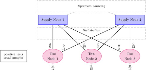
An illustrative example in Figure 1 depicts a tracked supply chain with three test nodes and two supply nodes. A supply node b-test node a path, also called an $(a,b)$ arc, is the product route from supply node b of $\mathcal{B}$ to test node a of $\mathcal{A}.$ Fraction labels indicate the number of positive tests over the total tests. A regulator only inspecting aggregate values at the test-node echelon may conclude that Test Nodes 1 and 2 are significant sources of SFP generation, given their positivity rates. However, products at these nodes only test positive when sourced from Supply Node 1. Half of the tested products from Supply Node 1 are SFPs, whereas no SFPs are associated with Supply Node 2. If the test nodes were truly generating SFPs, a more even distribution of discovered SFPs across supply-node paths would be expected. It instead seems more reasonable that SFPs stem from upstream factors associated with Supply Node 1. This example illustrates the importance of supply-chain information for determining SFP sources.

Figure 1. Extending analysis of PMS test results by one additional upstream echelon. “Upstream sourcing” and “Distribution” signify supply-chain locations for which information is not considered.

3.3. Sources of uncertainty

We describe three key sources of uncertainty when inferring SFP sources using PMS. Fundamental unidentifiability refers to the inability to conclude the origin of an SFP upon its detection. Testing accuracy refers to the ability of testing tools to correctly detect SFPs. Untracked sampling refers to the case where the supply node associated with each test is known probabilistically.

3.3.1. Fundamental unidentifiability

There is an inherent inability to identify the sources of SFPs when sampling only at test nodes and not at supply nodes: it cannot be stated with certainty that SFP generation did or did not occur upstream in the supply chain.

3.3.2. Testing accuracy

Testing tools have an inherent sensitivity and specificity. Sensitivity refers to the probability of a positive test result given that the tested product is indeed an SFP, and specificity refers to the probability of a negative test result given that the tested product is not an SFP. Kovacs et al. (2014) identified 42 SFP testing technologies and noted sensitivity in the range of 78–100% and specificity in the range of 88–100%, although metrics for some technologies were not reported and testing accuracy can depend on the type of pharmaceutical being tested. The detected amount of SFPs may increase or decrease from the amount that would be detected with perfectly accurate testing tools, depending on the testing accuracy as well as the SFP rates in the supply chain.

3.3.3. Untracked samples

In the untracked setting, the supply node associated with a sample is unknown. It is assumed instead that for each test node, a distribution across supply nodes can be constructed through historical procurement data or other means. Modeling outlets as test nodes and intermediary distributors as supply nodes, for example, testing data can be integrated with outlet records of previous distributor transactions to form untracked PMS data. The likelihood that test node a in $\mathcal{A}$ procures from supply node b in $\mathcal{B}$ is called the sourcing probability of test node a from supply node b, and is captured by element ${\mathit{Q}}_{ab}$ in matrix $\mathit{Q}\in {[0,1]}^{\left|\mathcal{A}\right|\times \left|\mathcal{B}\right|}.$ Note $\mathit{Q}$ resembles the path-link incidence matrices reviewed in Section 2.2. The row vector corresponding to the set of sourcing probabilities for test node a is ${\mathit{Q}}_a.$ Thus in the untracked case, the sourcing probability vector ${\mathit{Q}}_a$ is known for each test node a.

4. Problems in SFP inference

This section defines likelihood functions for PMS data and establishes that tracked and untracked supply chains are unidentifiable.

4.1. Tracked and untracked likelihoods

Binary data $y_1,\dots ,y_n$ are obtained for samples from test nodes in $\mathcal{A}$ that are tested with a device with sensitivity $s\in [0,1]$ and specificity $r\in [0,1].$ Each sample is collected uniformly from all products at the test node, and products at test nodes are sourced from supply nodes according to sourcing-probability matrix $\mathit{Q}.$ Conditional on test node random variable $A_i=a_i$ for sample i, $b_i$ is a realization of random variable $B_i$ which is independently sampled according to the probabilities in row ${\mathit{Q}}_a.$ The overall set of testing data is represented by $\mathit{d}=(\mathit{y},\mathit{a},\mathit{b})$ in the tracked case, where $\mathit{y}=\{y_1,\dots ,y_n\}$ is the set of testing results, $\mathit{a}=\{a_1,\dots ,a_n\}$ is the set of test-node labels, and $\mathit{b}=\{b_1,\dots ,b_n\}$ is the set of supply-node labels. For the untracked case, $\mathit{d}=(\mathit{y},\mathit{a},\mathit{Q}).$ Test-node SFP rates are stored in vector $\eta =({\eta }_1,\dots ,{\eta }_{\left|\mathcal{A}\right|})\in {(0,1)}^{\left|\mathcal{A}\right|}$ and supply-node SFP rates are stored in vector $\theta =({\theta }_1,\dots ,{\theta }_{\left|\mathcal{B}\right|})\in {(0,1)}^{\left|\mathcal{B}\right|}.$ A node’s SFP rate denotes a constant proportion of products traversing the node that become SFP. As nodes signify real-world locations, SFP rates of exactly zero or one are not considered: a rate of zero implies a node incapable of error, whereas a rate of one implies a node only distributing SFPs.

In multi-echelon supply chains, SFPs can be generated at any echelon. In our modeling of two connected echelons, when we say that products become SFP at either the test node or the supply node, we mean that SFP generation occurs at the test node, at an upstream location associated with the supply node, or at the supply node itself.

The consolidated SFP rate of a sample denotes the probability that the sample is an SFP when accounting for SFP rates at test nodes as well as supply nodes. It suffices to consider only the test node-supply node paths where test nodes have a non-zero probability of sourcing from the supply node. Let $\mathcal{E}\subseteq \mathcal{A}\times \mathcal{B}$ be the set of $(a,b)$ arcs where ${\mathit{Q}}_{ab}>0$. The consolidated SFP rate of a tracked sample collected from an $(a,b)$ arc in $\mathcal{E}$ is (1) $$z_{ab}^{\star }(\eta ,\theta )={\eta }_a+(1-{\eta }_a){\theta }_b.$$(1)

The first term of (1)(1) $$z_{ab}^{\star }(\eta ,\theta )={\eta }_a+(1-{\eta }_a){\theta }_b.$$(1) corresponds to the test-node SFP rate and the second term corresponds to the supply-node SFP rate, adjusted for the test-node rate. This adjustment is necessary as an SFP cannot generate at both the test node and the supply node; we assume once a pharmaceutical is substandard or falsified, additional poor supply-chain conditions do not make the pharmaceutical less suited for consumption. Further, an SFP cannot be recovered into a non-SFP. The consolidated SFP rate of an untracked sample collected from test node a in $\mathcal{A}$ is (2) $$\begin{array}{cc}{z}_a^{\star }(\eta ,\theta )=\sum _{b\in \mathcal{B}}{\mathit{Q}}_{ab}{z}_{ab}^{\star }(\eta ,\theta )=\hfill & {\eta }_a+(1-{\eta }_a)\sum _{b\in \mathcal{B}}{\mathit{Q}}_{ab}{\theta }_b .\hfill \end{array}$$(2)

(Note $\sum _{b\in \mathcal{B}}{\mathit{Q}}_{ab}=1$ for all a.) In the untracked case, each supply node–test node path is weighted according to the sourcing probabilities.

The tracked and untracked contexts differ in the supply-chain information available, yet the expressions of SFP probability are similar. To simplify notation we use supply-chain trace k of $\mathcal{K}$ to denote the supply-chain information available at sample collection: k of $\mathcal{K}$ is an $(a,b)$ arc in the tracked case and test node a in the untracked case, where $\mathcal{K}$ represents $\mathcal{E}$ or $\mathcal{A},$ respectively. The summary of the underlying SFP generation accordingly lies with vector $z^{\star }(\eta ,\theta )$ of length $\left|\mathcal{K}\right|,$ where element $z_k^{\star }(\eta ,\theta )$ of $z^{\star }(\eta ,\theta )$ refers to $z_{ab}^{\star }(\eta ,\theta )$ for some $(a,b)$ arc in the tracked case and $z_a^{\star }(\eta ,\theta )$ for some test node a in the untracked case. Similarly, supply-chain trace $k_i$ associated with sample i refers to either arc $(a_i,b_i)$ in the tracked case or $a_i$ in the untracked case, and random variable $K_i$ is $(A_i,B_i)$ in the tracked case or $A_i$ in the untracked case.

Given sensitivity s and specificity r, the probability of a positive SFP test is $z_k(\eta ,\theta )=s{z}_k^{\star }(\eta ,\theta )+(1-r)(1-z_k^{\star }(\eta ,\theta ))$ for each k of $\mathcal{K}.$ The random variable $Y_i$ of test i with supply-chain trace $K_i=k_i$ is one with probability $z_{k_i}(\eta ,\theta )$ and zero otherwise. The log-likelihood of $(\eta ,\theta )$ under data $\mathit{d}$ is (3) $$\mathcal{\ell }(\eta ,\theta |\mathit{d})=\sum _{i=1}^n[\hspace{0.17em}\log [z_{k_i}(\eta ,\theta )]y_i+\hspace{0.17em}\log [1-z_{k_i}(\eta ,\theta )](1-y_i)].$$(3)

The log-likelihood has a clearer form when summed over supply-chain traces in $\mathcal{K}.$ Let ${\mathcal{I}}_k=\left\{i\in \{1,\dots ,n\}:k_i=k\right\}$ be the tests corresponding to k. The number of results for k is $n_k=\left|{\mathcal{I}}_k\right|,$ with mean positive test rate of ${\overline{z}}_k=\frac{1}{n_k}\sum _{i\in {\mathcal{I}}_k}{y}_i.$ The log-likelihood in (3)(3) $$\mathcal{\ell }(\eta ,\theta |\mathit{d})=\sum _{i=1}^n[\hspace{0.17em}\log [z_{k_i}(\eta ,\theta )]y_i+\hspace{0.17em}\log [1-z_{k_i}(\eta ,\theta )](1-y_i)].$$(3) is equivalently expressed using $n_k$ and ${\overline{z}}_k$ as (4) $$\mathcal{\ell }(\eta ,\theta |\mathit{d})=\sum _{k\in \mathcal{K}}{n}_k[\log [z_k(\eta ,\theta )]{\overline{z}}_k+\hspace{0.17em}\log [1-z_k(\eta ,\theta )](1-{\overline{z}}_k)].$$(4)

Thus, the ${\overline{z}}_k$ and $n_k$ values across all k in $\mathcal{K}$ are sufficient statistics for the supply-chain traces of the data, as the likelihood can be expressed using these values without other data elements. As a result, the likelihood can be computed using a summary of PMS testing results. A usable PMS summary requires the number of positives and negatives associated with each supply-chain trace.

4.2. Unidentifiability

The tracked and untracked likelihoods are unidentifiable, i.e., for any set of SFP rates $(\eta ,\theta )$ there exists another set of SFP rates $({\eta }^{\prime },{\theta }^{\prime })$ such that $\mathcal{\ell }({\eta }^{\prime },{\theta }^{\prime }|\mathit{d})=\mathcal{\ell }(\eta ,\theta |\mathit{d}).$ Unidentifiability means data collection cannot uniquely reveal SFP rates. Theorems 1 and 2 state that unidentifiability is assured in the tracked and untracked cases for any set of testing data. Proofs are in Appendix A.

Theorem 1

(Tracked unidentifiability).

Let $(\eta ,\theta )$ be any set of SFP rates and let $\mathit{d}=(\mathit{y},\mathit{a},\mathit{b})$ be a set of tracked data. There exists $({\eta }^{\prime },{\theta }^{\prime })\ne (\eta ,\theta )$ such that $$\mathcal{\ell }({\eta }^{\prime },{\theta }^{\prime }|\mathit{d})=\mathcal{\ell }(\eta ,\theta |\mathit{d}).$$

Theorem 2

(Untracked unidentifiability).

Let $(\eta ,\theta )$ be any set of SFP rates and let $\mathit{d}=(\mathit{y},\mathit{a},\mathit{Q})$ be a set of untracked data. There exists $({\eta }^{\prime },{\theta }^{\prime })\ne (\eta ,\theta )$ such that $$\mathcal{\ell }({\eta }^{\prime },{\theta }^{\prime }|\mathit{d})=\mathcal{\ell }(\eta ,\theta |\mathit{d}).$$

Establishing unidentifiability in supply-chain PMS is a core contribution. We show unidentifiability exists when only considering two echelons of a supply chain; a corollary is that consideration of additional echelons also implies unidentifiability challenges. Thus, SFP rates cannot be recovered through PMS as currently practiced. Unidentifiability indicates a need for approaches that distinguish among multiple explanations for a set of data; Section 5 presents such an approach.

5. SFP-inference resolution

Theorems 1 and 2 show that identification of unique SFP rates explaining PMS data is not possible; yet, unidentifiability does not eliminate prospects for inferring SFP sources. This section presents a Bayesian approach to statistical inference of SFP rates that mitigates identifiability issues.

5.1. Bayesian mitigation of unidentifiability

Bayesian analysis combines observations and prior beliefs to infer unknowns. Placing priors on $(\eta ,\theta )$ encodes beliefs about SFP generation that distinguish candidate SFP rates with similar likelihoods. For example, Tebaldi and West (1998) employed a Bayesian approach to alleviate identifiability issues for pair-wise traffic counts for nodes in a network. Given different vectors of SFP rates with similar likelihoods under a set of PMS data and supply-chain information, prior expectations of the level and dispersal of SFPs across the supply chain help discern plausible vectors of SFP rates.

Let $p(\eta ,\theta )$ be a prior density on $(\eta ,\theta ).$ Multiplying $p(\eta ,\theta )$ with the likelihood under data $\mathit{d},$ $\hspace{0.17em}\exp \hspace{0.17em}(\mathcal{\ell }(\eta ,\theta |\mathit{d})),$ is then proportional to the posterior, i.e., (5) $$p(\eta ,\theta |\mathit{d})\propto \hspace{0.17em}\exp \hspace{0.17em}(\mathcal{\ell }(\eta ,\theta |\mathit{d}))p(\eta ,\theta ) .$$(5)

Posterior concentration at a region of high SFP rates for a particular node means that available information indicate that node as a credible SFP source. Posterior concentration at a region of low SFP rates indicates that node is not a credible SFP source. Non-concentration of the posterior means data are insufficient to overcome sources of uncertainty.

Sections 5.4 and 5.5 discuss prior formation and generating suitable posterior draws. Sections 5.2 and 5.3 first illustrate the application of inference in a PMS context.

5.2. Inference example

We revisit the example from Section 3.2 from a Bayesian perspective. Suppose one believes that SFP rates at nodes are independent and, although nodes could exhibit SFP rates near 40%, most nodes will exhibit SFP rates below 20%. A prior that meets this criterion on test-node SFP rates $\eta =({\eta }_1,{\eta }_2,{\eta }_3)$ and supply-node SFP rates $\theta =({\theta }_1,{\theta }_2)$ is $$p(\eta ,\theta )\propto \prod _{a\in \{1,2,3\}}\hspace{0.17em}\exp \hspace{0.17em}\left\{-\frac{1}{2}{\left[g({\eta }_a)+2\right]}^2\right\}\prod _{b\in \{1,2\}}\hspace{0.17em}\exp \hspace{0.17em}\left\{-\frac{1}{2}{\left[g({\theta }_b)+2\right]}^2\right\},$$ where $g(x)=\hspace{0.17em}\log \hspace{0.17em}\left(\frac{x}{1-x}\right)$ is the logit function. Using the logit transformation moves analysis to the real number line: manipulation of the posterior on the real number line avoids computational issues that arise as SFP rates approach zero or one.

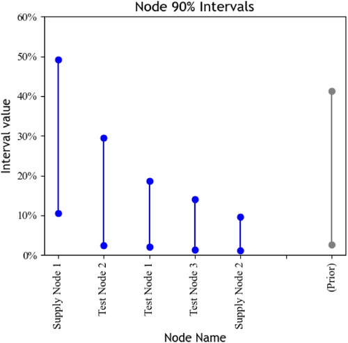
Combining the prior with the likelihood under the testing data from Figure 1 yields the posterior. Figure 2 depicts the 5% and 95% quantiles for 1,000 posterior draws of $(\eta ,\theta ).$ The quantiles for the prior are included for reference. A node associated with sufficiently high 5% quantiles indicates a significant posterior probability that SFP generation is linked with that node. For instance, Supply Node 1 likely constitutes a high SFP risk. However, although 9 of 20 tests associated with Supply Node 1 are SFPs (45%), the prior and the chance that the test nodes are responsible for some SFP generation mean that most weight for the interval for Supply Node 1 falls below the raw percentage of 45%. A high 95% quantile means that sufficient data may show the associated node to be a large driver of SFPs. For example, Test Node 2 has a 95% quantile near 30%: more data collection may plausibly show that Test Node 2 is associated with a higher SFP rate than Supply Node 1.

Figure 2. 5% and 95% quantiles for the posterior of example testing data in Figure 1.

5.3. Interpreting posterior samples

Draws from the posterior are used to build credible regions for the values of $(\eta ,\theta )$ that generated the data $\mathit{d}.$ Credible regions signify a space of SFP rates with ($1-\alpha$) posterior probability, for some desired $\alpha$ level. For example, the 5% and 95% quantiles are used to build a 90% interval. Wide intervals for particular nodes indicate that data are insufficient to draw conclusions. Drivers of inconclusive intervals include low sample size and the uncertainty sources of Section 3.3.

Interval interpretation should consider at least three categories for the application of regulatory resources. Similar to the thresholds of the lot-quality assurance sampling approach of Newton et al. (2009), categorization of nodes along the lines of “act,” “do not act,” and “gather more data before deciding,” allows regulators to translate PMS results into the allocation of intervention resources or further PMS activities. Categorization aids efficient use of limited resources under uncertainty.

We suggest using acceptance thresholds to build categories from posterior intervals. The first category includes nodes with interval lower bounds above some lower threshold l, where l signifies an SFP rate that triggers the use of further intervention resources. Data are sufficient to suggest that the SFP rates associated with members of this first category are as high as l. If the example in Figure 2 uses $l=5\%,$ then Supply Node 1 is categorized as a high SFP risk. Designation of l by regulators should consider the availability of intervention resources as well as what SFP rates are unacceptable in their domains. For instance, Newton et al. (2009) noted WHO guidelines for malaria programs that suggest a change in policy once treatment failure exceeds 10%; similar treatment-specific rates may guide designation of l for different pharmaceuticals.

The second category includes nodes with interval lower bounds below l, but upper bounds above an upper threshold u. SFP rates for members of this category are potentially as high as u, but more data are required to assert that SFP rates are not below l. Thus, targeting further PMS sampling of these nodes may be recommended. If the example in Figure 2 uses $l=5\%$ and $u=20\%,$ then Test Node 2 is a moderate SFP risk. Designation of u by regulators should consider what additional resources can be expended in investigating nodes with the potential for high SFP rates: setting u too low means potentially categorizing all nodes as moderate SFP risks.

The third category captures nodes associated with intervals that have upper bounds below u and lower bounds below l. Nodes in this category are least likely to pose significant SFP risk.

5.4. Prior formation

A variety of prior forms can be used with (5)(5) $$p(\eta ,\theta |\mathit{d})\propto \hspace{0.17em}\exp \hspace{0.17em}(\mathcal{\ell }(\eta ,\theta |\mathit{d}))p(\eta ,\theta ) .$$(5) . Effective priors encode regulator expectations of SFP generation with respect to size, variability, and dispersal pattern. Priors are beneficial for mitigating unidentifiability when informed by reliable regulatory domain knowledge.

Applications including the modeling of movie sales and interventions against infections have employed density transformations to enable application-specific analysis (Ainslie, et al., 2005; Hui et al., 2020). Similarly, an effective strategy here is developing priors on the real number line and transforming the resulting posterior SFP rates to the $(0,1)$ interval for analysis. Priors defined on the real number line also favorably correspond with the SFP rates indicated by studies in the literature: the resulting distributions have long tails, which aligns with the heterogeneity of SFP generation noted by WHO (2017b).

Consider an independent normal prior, expressed as $$p(\eta ,\theta )\propto \prod _{a\in \mathcal{A}}\hspace{0.17em}\exp \hspace{0.17em}\left\{-\frac{1}{2}{\left[\frac{g({\eta }_a)-\gamma }{\nu }\right]}^2\right\}\prod _{b\in \mathcal{B}}\hspace{0.17em}\exp \hspace{0.17em}\left\{-\frac{1}{2}{\left[\frac{g({\theta }_b)-\gamma }{\nu }\right]}^2\right\}.$$

Parameter $\gamma$ signifies a prior belief of the standard SFP rate at test nodes and supply nodes, and $\nu$ corresponds to SFP-rate spread. The standard parameter centers expectations of SFP prevalence throughout the supply chain. The spread parameter reflects the anticipated variety across rates. For example, a normal prior on the real number line with $\gamma =-2$ and $\nu =1$ produces a distribution in the $(0,1)$ space with respective 5%, 50% and 95% quantiles of 3%, 12% and 41%.

For low $\gamma$ values, the independence within each prior reflects an assumption that it is unlikely that many SFP sources exist: one node carrying an SFP rate above $\gamma$ has higher prior likelihood than many nodes carrying such SFP rates. Using priors with lower spread parameters requires more testing data to pull the posterior probability towards regions favored by the likelihood.

Consider an independent Laplace prior, which carries a similar shape to the normal: $$p(\eta ,\theta )\propto \prod _{a\in \mathcal{A}}\hspace{0.17em}\exp \hspace{0.17em}\left\{-\frac{|g({\eta }_a)-\gamma |}{\nu }\right\}\prod _{b\in \mathcal{B}}\hspace{0.17em}\exp \hspace{0.17em}\left\{-\frac{|g({\theta }_b)-\gamma |}{\nu }\right\}.$$

For average and spread similar to the normal, an independent Laplace concentrates nearer the average and has heavier tails. A Laplace prior reflects an anticipation that some nodes will have SFP rates far from the average; thus the Laplace may better suit consideration of falsification, where falsifiers exploit available, yet limited, entry points (WHO, 2017b). A normal prior reflects an expectation that rates will vary nearer the average; thus the normal may better suit substandardization: production, transportation and storage entail similar activities conducted by different actors.

5.5. Markov chain Monte Carlo sampling

To build the inference described in Section 5.3, samples from the posterior are needed. The posterior in (5)(5) $$p(\eta ,\theta |\mathit{d})\propto \hspace{0.17em}\exp \hspace{0.17em}(\mathcal{\ell }(\eta ,\theta |\mathit{d}))p(\eta ,\theta ) .$$(5) does not exhibit natural sampling, but tools such as Markov chain Monte Carlo (MCMC) allow sampling from general posteriors. Our study uses the No-U-Turn Sampler (NUTS) sampler of Hoffman and Gelman (2014). This sampler uses posterior gradient information; Supplementary Material I contains applicable posterior derivatives. The NUTS sampler requires a number of samples to warm start, as well as a parameter, $\delta ,$ that governs how the algorithm proposes samples. Our analysis uses $\delta$ of 0.4, which falls within the region suggested by Hoffman and Gelman (2014) The analysis then generates 5,000 warm-start draws and 1,000 draws for inference; more inference draws could be used, but 1,000 draws appear sufficient for analysis (see Supplemental Material II).

Computation time is not a major restriction for analyzing data common to many low- and middle-income settings. Supplementary Material II describes drivers of computation time. In general, more nodes increases the dimensionality of $(\eta ,\theta )$ and slows down sampling. However, computation time for a system with 100 nodes is seconds, and supply chains in most cases will not feature more than a few hundred nodes. Our code is publicly available on Github as Python package logistigate (Wickett et al., 2021).

6. Case study

Several national regulatory agencies in low- and middle-income countries provide data to United States Pharmacopeia’s MQDB to strengthen global regulatory capacity. We use a PMS data set from MQDB to show how incorporating upstream information can add to the understanding of SFP sources. The case study demonstrates unidentifiability in real PMS data and shows the value of our Bayesian approach over current practice.

6.1. Case-study setting

The data consist of products collected and tested by a country’s pharmaceutical regulatory agency in 2010. The data are anonymized to protect the country’s sources and mask the outlets and manufacturers involved. A data record denotes purchasing and testing information for a single form of a pharmaceutical product as sold to consumers, e.g., a box of 12 tablets. A test result is either “Pass,” meaning compliance with registration specification, or “Fail,” meaning non-compliance. Each record is associated with multiple geographic divisions. We consider the “District” and “Manufacturer” levels of the supply chain, where District refers to the second-largest geographic sub-division of the country. We model Manufacturers as supply nodes and Districts as test nodes.

The case-study data feature 25 Manufacturers and 23 Districts in 406 PMS records. These data contain 73 positive tests, or an 18% SFP rate. An 18% SFP rate suggests significant quality issues for the areas sampled by regulators; however, examination of the testing results by only supply-node or test-node label reveals difficulties in defining SFP sources. District 8 features seven SFPs of 12 associated tests (58%), District 7 features 24 SFPs of 81 tests (30%), and District 16 features eight SFPs of 44 tests (18%). A natural regulatory response would be to dedicate intervention resources to these districts with SFP rates exceeding the national average of 18%. At the same time, 8 of 21 samples from Manufacturer 8 are SFPs (38%), 28 of 92 samples from Manufacturer 5 are SFPs (30%), and 5 of 31 samples from Manufacturer 3 are SFPs (16%). Examining data by manufacturer, a justifiable regulatory response would be to dedicate resources to investigating supply-chain factors associated with these manufacturers.

6.2. Limitations of current methods

Lot-quality assurance described in Newton et al. (2009) uses standard 90% confidence intervals for proportions to determine if SFP prevalence for a node exceeds quality thresholds, where the 90% interval for a given proportion $\widehat{z}$ and number of samples $n_{\widehat{z}}$ is given as $\widehat{z}\pm 1.645\sqrt{\widehat{z}(1-\widehat{z})/n_{\widehat{z}}}.$ The proportion $\widehat{z}$ can relate to either a test node or a supply node. For instance, the standard interval for Manufacturer 13 is $(7\%,22\%)$ and the standard interval for District 5 is $(5\%,25\%).$ The intervals for six districts and eight manufacturers exceed a threshold of $l=5\%.$ A typical regulator response would be to allocate investigative and intervention resources to these locations.

Additionally, a common requirement for the standard interval is $n_{\widehat{z}}\widehat{z}\ge 5$ and $n_{\widehat{z}}(1-\widehat{z})\ge 5$ (Mann, 2010). In this data set, the requirement is satisfied by only 5 of 25 manufacturers and 6 of 23 districts. Obtaining sufficient tests for all test and supply nodes may be infeasible in many resource-limited settings, as in our experiences at USP: regulators must often allocate resources using insufficient numbers of tests. In contrast, our method does not have a minimum to complete inference; Manufacturer 2, for example, is featured on only one test.

6.3. Manufacturer–district analysis

The expectations grounding the prior in the Manufacturer–District analysis follows past work in PMS. Previous studies, such as those reviewed in Ozawa et al. (2018), typically reported aggregated rates across countries, geographic regions, or sub-divisions of the pharmaceutical market. Research shows that although SFPs are a widespread global problem, SFP generation is heterogeneous: much of the supply chain exhibits low rates while many SFPs derive from a few supply-chain locations (UNICRI, 2012; WHO, 2017b). Thus the prior for analysis employs an average SFP rate anchored to what previous studies indicate and a spread sufficiently high to capture anticipated heterogeneity. An independent Laplace prior with average $\gamma =-2.5$ and spread parameter $\nu =1.3$ produces an average of 15%, a median of 8%, and a 90% interval of [0.4%, 62%], meaning the prior carries a long right tail covering high SFP-rate regions. In fact, 70% of prior weight falls below an SFP rate of 14%. The sensitivity analysis in Supplementary Material III indicates that prior choice does not have an instrumental effect on interval width; sufficient data seem to counterbalance the prior designation.

The Manufacturer–District analysis assumes perfect testing sensitivity and specificity to enable easier isolation of the effects of fundamental unidentifiability and untracked settings. As expected, sensitivity analysis shows that testing-tool uncertainty generally has an inflationary effect on inference; this inflationary effect is larger for nodes for which there are less data.

Figures 3 and 4 show 90% intervals for SFP rates corresponding to Districts and Manufacturers, respectively, under both tracked and untracked settings. (Figure 4 is in Appendix B.) The figures use the classification scheme described in Section 5.3 with $l=5\%$ and $u=30\%.$ First, consider the tracked setting. Our method’s credible intervals are comparable in width with the standard intervals described in Section 6.2; however, as SFP rates are not considered across the supply chain, the standard intervals are shifted higher by 10 to 30%. Let the raw SFP rate of a given node be the SFP rate of all tests associated with that node, despite the upstream or downstream supply-chain factors causing SFPs. Raw rates only apply to supply nodes in the tracked case, as the supply node for each test is unknown in the untracked case. The raw SFP rates for samples from Manufacturers 10, 8, and 5 are 57%, 38%, and 34%, respectively, and the raw rates associated with District 8 and 7 are respectively 58% and 30%. The raw SFP rates sit near the interval upper bounds for each Manufacturer and District; the interval upper bound for Manufacturer 5, for instance, is 38%. The intervals skew lower than the raw rates for all nodes. The posterior constituting these intervals is accounting for a prior with a low average, in addition to the possibility that SFPs are generated at either test nodes or supply nodes. In addition, our method reflects uncertainty from low levels of data. For instance, Manufacturer 2 has only one associated (positive) test: the associated interval spans most of $(0\%,100\%).$

Figure 3. Test-node and supply-node 90% intervals for MCMC samples generated using case-study data in the tracked setting. Intervals with lower bounds above $l=5\%$ are featured in solid lines on the left, intervals with lower bounds below l and upper bounds above $u=30\%$ are featured in dashed lines in the middle, and all other intervals are featured in dotted lines on the right.

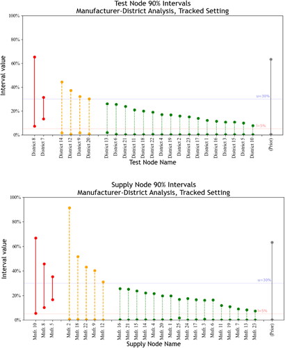
Figure 4. Test-node and supply-node 90% intervals for MCMC samples generated using case-study data in the tracked setting. Intervals with lower bounds above $l=5\%$ are featured in solid lines on the left, intervals with lower bounds below l and upper bounds above $u=30\%$ are featured in dashed lines in the middle, and all other intervals are featured in dotted lines on the right.

Direct consideration of supply-chain connections and associated testing data lends credence to the inferences illustrated in the figures. All seven SFPs associated with District 8 are tied to Manufacturers with at least 15% raw SFP rates: Manufacturers 3, 5, 8, 10 and 24. The data also feature four non-SFPs for tests from the District 8-Manufacturer 13 arc, which does not support District 8 as a major SFP source. District 7, on the other hand, is associated with 19 tests featuring Manufacturer 13, where eight of these tests are SFPs (42%). The other 43 tests involving Manufacturer 13 feature only one SFP; thus, District 7 is likely a significant SFP source. The standard interval for Manufacturer 13 is $(7\%,22\%),$ while our method’s interval for Manufacturer 13 is (0.1%, 9%). A regulator using the standard interval under $l=5\%$ would find Manufacturer 13 to be associated with significant SFP sources. Thus, we observe how the posterior addresses the challenge of fundamental unidentifiability by integrating testing data, supply-chain information, and prior expectations to create credible intervals that regulators can use to improve policy decisions.

The analysis also illustrates the importance of supply-chain connections for forming inferences in the tracked setting: without interconnected nodes, fundamental unidentifiability renders too many SFP scenarios as plausible. Sourcing patterns limit the number of scenarios that can credibly explain the data. The interval associated with District 5 is an example of the importance of sourcing patterns. Although testing at District 5 yields five SFPs in 34 samples (15%), District 5 has a narrower interval than the interval for District 17, which yields no SFPs in nine samples. Inspection of the manufacturers associated with District 5 samples reveals that all five SFPs are sourced from Manufacturer 5. The standard interval for District 5 is $(5\%,25\%),$ exceeding the lower threshold of $l=5\%,$ while our method’s credible interval for District 5 is (2%, 9%). Instead of suspecting SFP generation at District 5, supply-chain information allows us to infer the opposite: District 5 is less likely an SFP source than another test node, District 17, with no detected SFPs. A regulator using standard intervals may invest intervention resources in District 5, whereas incorporating supply-chain information avoids this investment. Thus, the inferences resulting from our approach can help regulators determine if data are sufficient to invest limited regulatory resources.

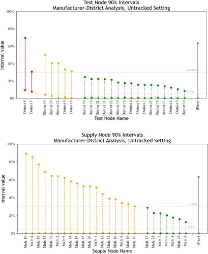
For the untracked setting, the sourcing-probability matrix, $\mathit{Q},$ is used as the supply-chain trace instead of the supply-node labels. The estimated element of $\mathit{Q}$ corresponding to District a and Manufacturer b is formed by dividing the number of observed samples from arc $(a,b)$ by the total number of samples collected from test node a. The resulting matrix is sparse: test nodes only source from a subset of supply nodes. Comparing the tracked and untracked intervals, as shown in Figures 3 and 4, reveals the value of tracked over untracked information. The intervals associated with test nodes remain nearly identical, whereas the intervals associated with supply nodes change considerably. This effect is reasonable: we know test nodes exactly and supply nodes only probabilistically. The untracked supply-node intervals still indicate that upstream supply-chain factors are associated with SFP generation, as shown by the many Manufacturers classified as moderate risks. However, inferring the most critical upstream direction from many options is unclear. Untracked analysis for this case study thus carries Type II risk, where potential upstream sources of SFP are missed.

In the untracked case, the structure of $\mathit{Q}$ is an important factor in the ability to overcome unidentifiability. In particular, untracked inference is hampered when test nodes possess similar sourcing patterns. For instance, 18 of 23 Districts had more than 10% of associated tests tied to Manufacturer 5. SFPs associated with upstream supply-chain factors become difficult to infer. Even if it is known that upstream factors are principal SFP drivers, SFPs can just as likely stem from a supply node with high market share and a low SFP rate as from a supply node with low market share and a high SFP rate. Accordingly, the ideal sourcing environment for successful untracked inference is an environment where each test node sources from a small subset of supply nodes, with only a few shared supply nodes among any subset of test nodes.

Another challenge to untracked inference is sufficiently estimating the sourcing structure from past data. Estimating $\mathit{Q}$ from procurement or sourcing records carries variance due to the sampling variance of the records. Supplementary Material III examines inference sensitivity to the estimation of $\mathit{Q}$ using bootstrap sampling; use of different $\mathit{Q}$ estimates for this case study impacts the resulting inference for supply nodes but not for test nodes. In sum, untracked settings carry challenges for inferring upstream SFP sources, particularly if information for estimating $\mathit{Q}$ is too limited.

7. Conclusion and discussion

Regulators in low- and middle-income countries can benefit from new tools and methods to maximize the power of surveillance activities. This article characterizes the challenge of identifying SFP sources under PMS and demonstrates how the analytical capacity of PMS can be expanded by consideration of supply-chain information. Our case study illustrates how a Bayesian approach can be combined with domain expertise through well-chosen priors to strengthen identification of SFP sources. PMS data, including upstream supply-chain information, are already collected routinely; this article provides a means of extracting more utility from this regular activity.

In addition to limited budgets, the WHO has identified poor international coordination as a significant challenge for regulators in low- and middle-income countries (WHO, 2017b). Placing PMS in a supply-chain context opens avenues for collaboration among regulators in different countries with overlapping supply chains. As scanning and tracking technology becomes more widely available, the collection of additional supply-chain information presents more opportunities for identifying quality issues. Our analysis shows the value of additional supply-chain information.

7.1. Implementation guidelines

Implementation of the approach will be accompanied by challenges. In addition to low overall numbers of tests, supply-chain information in current PMS collection records can be limited, and this information is crucial to identifying supply chain-driven problems. Standard PMS may benefit from supplementing the data-collection checklist proposed by Newton et al. (2009), MEDQUARG, with key supply-chain information such as importers, warehouses, and intermediaries. Furthermore, proper accounting of the uncertainty associated with a PMS test requires known sensitivity and specificity with respect to the testing tool. Testing-tool accuracy can vary by therapeutic indication, e.g., antimalarial, or by technician experience, and thus sensitivity and specificity should be recorded for each test where possible. In particular, false positives in low-SFP environments have the potential to confuse analysis and lead to unproductive use of resources.

The adaptable designation of nodes as individual locations or aggregates of such locations, as well as the designation of supply nodes as locations in any upstream echelon, are features that allow generalization of our approach to many low- and middle-income countries. The supply-chain information available to regulators is often constrained; the only requirements of our approach are standard test node labels and information, even if partial, about some upstream echelon. Additionally, the variety in SFP causes requires adaptable methods. For instance, economic conditions in one region may encourage a higher prevalence of falsified products in that region, or choices by one plant manager may result in a higher rate of substandard products. Our approach allows for different analyses using individual supply-chain locations or aggregates of such locations to match goals. The value of this adaptability is illustrated in our case study, which infers notable aggregate District SFP rates as well as SFP rates associated with individual Manufacturers.

Implementation may require customized deployments in different settings. For instance, some settings may feature tracked, as well as untracked, supply-chain information; for example, scanning records may be available at every transferal point for public-sector products, whereas only procurement records are available for private-sector or non-profit, non-governmental products. In this case, each test i has an associated trace $k_i$ that is either tracked or untracked, and the vector of sourcing probabilities for untracked samples is available. Thus, the log-likelihood of (4)(4) $$\mathcal{\ell }(\eta ,\theta |\mathit{d})=\sum _{k\in \mathcal{K}}{n}_k[\log [z_k(\eta ,\theta )]{\overline{z}}_k+\hspace{0.17em}\log [1-z_k(\eta ,\theta )](1-{\overline{z}}_k)].$$(4) , $$\mathcal{\ell }(\eta ,\theta |\mathit{d})=\sum _{i=1}^n[\hspace{0.17em}\log [z_{k_i}(\eta ,\theta )]y_i+\hspace{0.17em}\log [1-z_{k_i}(\eta ,\theta )](1-y_i)],$$ can be constructed through the corresponding $k_i$ of each test, and inference can be conducted as described in Section 5. Prior construction is another fundamental element of our approach involving some ambiguity. Section 6.3 forms a prior using studies from the global literature on SFPs; using the global to characterize the local may be inadvisable in some environments. Section 5 suggests independent priors to capture the notion that SFP generation at one node does not affect generation at other nodes. However, it is feasible that changes in regulatory environments might stimulate correlated SFP behavior across nodes: Eban (2019) discussed “two-tracked” manufacturers with different supply lines for high-income and low-income countries. Improved prior formation that captures local features requires an interaction between practitioners and statisticians.

In this work, the distinction between substandard and falsified is not instrumental. “SFP” is broadly used to refer to products unsuitable for consumption. We consider an environment where SFPs frequently occur, test results are captured by a binary variable, and the aim is to better understand SFP sources. Although the WHO includes unregistered products in its definition of poor quality (WHO, 2018), our study concentrates on substandard and falsified products—the principal focus of the literature on poor-quality medical products. Substandard and falsified products generally have different generation mechanisms (WHO, 2017b); however, both substandard and falsified products are problems rooted in supply-chain conditions (Pisani et al., 2019). Usual PMS implementation seeks detection of all causes of poor quality simultaneously, and often does not require different diagnostics for each cause. Regulators can select the criteria with which tests are marked as positive or negative. Depending on objectives and detection tools, one may consider only substandard products, only falsified products, all SFPs, or even unregistered products.

The approach of this article only considers binary pass–fail measurements, consistent with data in MQDB. Due to the affordability and flexibility of screening tests, PMS data can consist largely of pass–fail results. Regulators can conduct a single screening test with minimal training for less than a dollar per test, while running high-powered testing requires reference standards, training, and technology costing upwards of hundreds of thousands of dollars (Kovacs et al., 2014; Chen et al., 2021). Further, pharmaceuticals have different stability profiles. Products may fail testing for any quality attribute, such as dissolution characteristics or impurity prevalence; however, proportions of expected Active Pharmaceutical Ingredients, or API, are the most widely measured. API content can be measured through common non-laboratory methods and provide important information regarding SFP causes (WHO, 2017b). For instance, large discrepancies with the declared content often indicate falsified products. A testing failure due to detected API content that is 4% outside the acceptable range implies different causes than a failure with detected API content that is 70% below the acceptable range. The first failure is generally associated with substandard products, whereas the second failure is expected with falsified products. Keeping with the binary response variable, falsified and substandard products could be categorized using different API thresholds. However, full analysis of API requires modeling the pharmaceutical-degradation process and integrating stability behavior with supply-chain information. Moving to an inference model that treats API content as a continuous response variable would be a valuable line of future research.

7.2. Broader objectives

This method can assist in the selection of testing methodology—assessing, for example, if it is better to run 1,000 tests with a spectrometer or 10,000 tests with thin-layer chromotography. The consideration of costs versus accuracy within an inferential context could be leveraged to explore scenarios where an inexpensive, less accurate testing tool is preferential to an expensive, highly accurate testing tool, as explored in Chen et al. (2021).

The method can also inform the collection of additional samples. If the interval for a particular test node is sufficiently narrow, allocating samples to different test nodes may be recommended. Alternatively, if more data are desired regarding a particular supply node, sampling from a test node with a narrow interval may be sensible if the supply node is often sourced by the test node. Integration of statistical methods with regulatory insights and objectives can inform an adaptive sampling framework that feeds testing results into sample allocation decisions. Sequential analysis, which determines stopping rules for when data sufficient for regulator objectives have been collected, and Bayesian experiment design, which seeks to maximize the inference utility through sampling choices, may be valuable avenues. An adaptive sampling framework may also forgo the assumption that elements such as $(\eta ,\theta )$ or $\mathit{Q}$ are constant, and signal when these elements have significantly shifted. Understanding how PMS data may be analyzed is a crucial step towards using available supply-chain information to guide the choice of sampling locations.

Additional supply-chain echelons can be integrated into the log-likelihood if supply-chain information from multiple echelons is available. Consider a tracked case where each test bears a label for a node from an additional echelon of distributor nodes sitting between supply nodes and test nodes. Let $\mathcal{C}$ be the set of distributor nodes with corresponding SFP rates $\zeta =({\zeta }_1,\dots ,{\zeta }_{\left|\mathcal{C}\right|}).$ The consolidated SFP rate of a test from a supply node b-distributor node c-test node a path is then (6) $$z_{\mathit{acb}}^{\star }(\eta ,\zeta ,\theta )={\eta }_a+(1-{\eta }_a)z_{cb}^{\star }(\zeta ,\theta ) .$$(6)

Thus, the log-likelihood of (4)(4) $$\mathcal{\ell }(\eta ,\theta |\mathit{d})=\sum _{k\in \mathcal{K}}{n}_k[\log [z_k(\eta ,\theta )]{\overline{z}}_k+\hspace{0.17em}\log [1-z_k(\eta ,\theta )](1-{\overline{z}}_k)].$$(4) can be constructed by using trace $k_i=(a_i,c_i,b_i)$ for each test i. The consolidated SFP rate in the untracked case can be similarly formed. Although tests with more than two labels are not explored in this article, magnified unidentifiability issues should be anticipated when considering more than two echelons, as additional SFP rates are being inferred without additional testing data. In a context where testing data are available from multiple echelons, future work can ascertain the conditions for identifiability or unidentifiability of SFP rates.

An additional managerial implication concerns the pooling of quality-assurance resources internationally. The global nature of pharmaceutical supply chains means SFPs may generate between manufacture and domestic introduction. Integrating information across borders provides the possibility for studying complex, multi-tiered supply chains that feature many echelons of interconnected nodes. Two countries with limited regulatory resources can expand their inferential power by sharing testing data and supply-chain information. Expanding the scope of our approach may also entail an improved modeling of manufacturing and black-market mechanisms, perhaps using insights from work such as Pisani et al. (2019). Information such as economic indicators may be incorporated into prior construction to better anticipate SFP generation.

Data availability statement

Due to the nature of this research, participants of this study did not agree for their data to be shared publicly; supporting data are not available. In lieu of data used in the case study, analogous synthetic data that permit similar findings can be found on Github at https://github.com/eugenewickett/inferringSFPsrepoducibilityreport.

Additional information

Funding

This work was funded through two National Science Foundation grants: EAGER Award 1842369: ISN: Unraveling Illicit Supply Chains for Falsified Pharmaceuticals with a Citizen Science Approach, and NSF 1953111. We acknowledge United States Pharmacopeial Convention (USP) and the Promoting the Quality of Medicines Plus (PQM+) program, funded by the United States Agency for International Development (USAID), for the use of data in our case study and the time of staff, including the co-authors, spent contributing to this paper.

Notes on contributors

Eugene Wickett

Eugene Wickett is a PhD candidate in Industrial Engineering and Management Sciences at Northwestern University. His dissertation considers the regulation of pharmaceutical supply chains.

Matthew Plumlee

Matthew Plumlee is an assistant professor in the Department of Industrial Engineering and Management Sciences at Northwestern University. He primarily studies uncertainty quantification methods for computational models of systems.

Karen Smilowitz

Karen Smilowitzis the James N. and Margie M. Krebs Professor in Industrial Engineering and Management Science at Northwestern University, with a joint appointment in the Operations group at the Kellogg School of Management. Dr. Smilowitz is an expert in modeling and solution approaches for logistics and transportation systems in both commercial and nonprofit applications. Dr. Smilowitz is the Editor-in-Chief of Transportation Science and a Fellow of the INFORMS society.

Souly Phanouvong

Souly Phanouvong is the Senior Technical Advisor, Regulatory Systems Strengthening for the USAIDfunded Promoting the Quality of Medicines Plus (PQM+) Program of the United States Pharmacopeial (USP) Convention. He has over 35+ years of national, regional, and international experience in medicines policy and regulations, quality assurance and quality control of medical products. He has contributed to regulatory capacity strengthening in over 15 countries in Asia and the Pacific, and some 13 countries in Africa. He holds a PharmD and two PhDs (from Budapest, Hungary; and Melbourne, Australia).

Victor Pribluda

Victor S. Pribluda is the Senior International Regulatory Intelligence Manager at the Global External Affair division at the United States Pharmacopeia since 2019, where he also oversees technical support tools and documentation for Post Marketing Surveillance. Dr. Pribluda earned his M. in Chemical Science from the National University of Buenos Aires, Argentina, and his PhD in Cellular Biology from the Weizmann Institute of Science, Rehovot, Israel.

Appendices to Inferring sources of substandard and falsified products in pharmaceutical supply chains by Wickett, Plumlee, Smilowitz, Phanouvong and Pribluda

Appendix A. Proofs

Proof of Theorem 1.

For original SFP rates $(\eta ,\theta )$ in the tracked setting, we form $({\eta }^{\prime },{\theta }^{\prime })\ne (\eta ,\theta )$ with an initial adjustment of the SFP rate at one test node by some $ϵ.$ We use the original rate at this test node and $ϵ$ to produce adjusted rates at all other nodes that result in $({\eta }^{\prime },{\theta }^{\prime })$ with the same likelihood as $(\eta ,\theta ).$

Let $(\eta ,\theta )$ be any set of SFP rates. Select test node $a^{\prime }$ and $ϵ>0.$ For each test node a, set ${\eta }_a^{\prime }$ as (7) $${\eta }_a^{\prime }={\eta }_a-ϵ\frac{1-{\eta }_a}{1-{\eta }_{a^{\prime }}},$$(7) and for each supply node b, set ${\theta }_b^{\prime }$ as (8) $${\theta }_b^{\prime }=\frac{{\theta }_b(1-{\eta }_{a^{\prime }})+ϵ}{1-{\eta }_{a^{\prime }}+ϵ}.$$(8) Inspection of (7)(7) $${\eta }_a^{\prime }={\eta }_a-ϵ\frac{1-{\eta }_a}{1-{\eta }_{a^{\prime }}},$$(7) reveals that a sufficiently small $ϵ$ assures ${\eta }_a^{\prime }>0$ for each a. For any $ϵ>0,$ inspection of (8)(8) $${\theta }_b^{\prime }=\frac{{\theta }_b(1-{\eta }_{a^{\prime }})+ϵ}{1-{\eta }_{a^{\prime }}+ϵ}.$$(8) shows that ${\theta }_b^{\prime }<1,$ as SFP rates are assumed to be between 0 and 1. Thus a sufficiently small $ϵ$ assures valid adjusted rates $({\eta }^{\prime },{\theta }^{\prime })$ such that $({\eta }^{\prime },{\theta }^{\prime })\ne (\eta ,\theta ).$

Consider the tracked consolidated SFP rate under $({\eta }^{\prime },{\theta }^{\prime })$ for any $(a,b)$ arc: $$\begin{array}{c}{z}_{ab}^{\star }({\eta }^{\prime },{\theta }^{\prime })={\eta }_a^{\prime }+(1-{\eta }_a^{\prime }){\theta }_b^{\prime }\\ ={\eta }_a-ϵ\frac{1-{\eta }_a}{1-{\eta }_{a^{\prime }}}+\left(1-{\eta }_a+ϵ\frac{1-{\eta }_a}{1-{\eta }_{a^{\prime }}}\right)\frac{{\theta }_b(1-{\eta }_{a^{\prime }})+ϵ}{1-{\eta }_{a^{\prime }}+ϵ}\\ ={\eta }_a-ϵ\frac{1-{\eta }_a}{1-{\eta }_{a^{\prime }}}+\left(\frac{(1-{\eta }_a)(1-{\eta }_{a^{\prime }}+ϵ)}{1-{\eta }_{a^{\prime }}}\right)\frac{{\theta }_b(1-{\eta }_{a^{\prime }})+ϵ}{1-{\eta }_{a^{\prime }}+ϵ}\\ ={\eta }_a+\frac{{\theta }_b(1-{\eta }_{a^{\prime }})-{\eta }_a{\theta }_b(1-{\eta }_{a^{\prime }})-ϵ+ϵ{\eta }_a+ϵ-ϵ{\eta }_a}{1-{\eta }_{a^{\prime }}}\\ ={\eta }_a+(1-{\eta }_a){\theta }_b=z_{ab}^{\star }(\eta ,\theta ) .\end{array}$$ Thus $z_{ab}^{\star }({\eta }^{\prime },{\theta }^{\prime })=z_{ab}^{\star }(\eta ,\theta )$ for all arcs and $\mathcal{\ell }({\eta }^{\prime },{\theta }^{\prime }|\mathit{d})=\mathcal{\ell }(\eta ,\theta |\mathit{d}).$ □

Proof of Theorem 2.

For original SFP rates $(\eta ,\theta )$ in a supply chain in the untracked setting, we form $({\eta }^{\prime },{\theta }^{\prime })\ne (\eta ,\theta )$ by adjusting the SFP rate at one supply node by some $ϵ.$ The SFP rates at all test nodes are then adjusted by an amount proportional to the respective sourcing probability of that supply node to produce $({\eta }^{\prime },{\theta }^{\prime })$ with the same likelihood as $(\eta ,\theta ).$

Let $(\eta ,\theta )$ be any set of SFP rates. Select a supply node b and choose $ϵ>0$ such that ${\mathit{Q}}_a(\theta -e_bϵ)>0$ for test node a, where ${\mathit{Q}}_a$ is the row vector of sourcing probabilities in $\mathit{Q}$ corresponding to a and $e_b$ is a vector of length $\left|\mathcal{B}\right|$ with a one at the bth element and a zero at all other elements. Such an $ϵ$ exists as all SFP-rates are non-zero. Set ${\theta }^{\prime }=\theta -e_bϵ.$ For each a, set ${\eta }_a^{\prime }$ as (9) $${\eta }_a^{\prime }=\frac{{\eta }_a(1-{\mathit{Q}}_a\theta )+ϵ{\mathit{Q}}_{ab}}{1-{\mathit{Q}}_a\theta +ϵ{\mathit{Q}}_{ab}} .$$(9) As the elements of each row ${\mathit{Q}}_a$ sum to one, it follows that ${\mathit{Q}}_a\theta <1.$ Additionally, since SFP rates and sourcing probabilities are all between zero and one, it holds that $0<{\eta }_a^{\prime }<1$ for any $ϵ>0,$ and thus $({\eta }^{\prime },{\theta }^{\prime })$ are valid rates. As ${\theta }_b^{\prime }={\theta }_b-ϵ$ for some $ϵ>0,$ it follows that $({\eta }^{\prime },{\theta }^{\prime })\ne (\eta ,\theta ).$

Consider the untracked consolidated SFP rate under $({\eta }^{\prime },{\theta }^{\prime })$ at any test node a: $$\begin{array}{cc}{z}_a^{\star }({\eta }^{\prime },{\theta }^{\prime })={\eta }_a^{\prime }+(1-{\eta }_a^{\prime }){\mathit{Q}}_a{\theta }^{\prime }\hfill & \hfill \\ =\frac{{\eta }_a(1-{\mathit{Q}}_a\theta )+ϵ{\mathit{Q}}_{ab}}{1-{\mathit{Q}}_a\theta +ϵ{\mathit{Q}}_{ab}}+\frac{(1-{\eta }_a)(1-{\mathit{Q}}_a\theta )}{1-{\mathit{Q}}_a\theta +ϵ{\mathit{Q}}_{ab}}{\mathit{Q}}_a(\theta -e_bϵ)\hfill & \hfill \\ =\frac{{\eta }_a(1-{\mathit{Q}}_a\theta )+{\mathit{Q}}_a\theta -{\mathit{Q}}_a\theta ({\mathit{Q}}_a\theta -ϵ{\mathit{Q}}_{ab})-{\eta }_a({\mathit{Q}}_a\theta -ϵ{\mathit{Q}}_{ab})+{\eta }_a{\mathit{Q}}_a\theta ({\mathit{Q}}_a\theta -ϵ{\mathit{Q}}_{ab})}{1-{\mathit{Q}}_a\theta +ϵ{\mathit{Q}}_{ab}}\hfill & \hfill \\ =\frac{{\eta }_a+(1-{\eta }_a){\mathit{Q}}_a\theta -{\mathit{Q}}_a\theta [{\eta }_a+(1-{\eta }_a){\mathit{Q}}_a\theta ]+ϵ{\mathit{Q}}_{ab}[{\eta }_a+(1-{\eta }_a){\mathit{Q}}_a\theta ]}{1-{\mathit{Q}}_a\theta +ϵ{\mathit{Q}}_{ab}}\hfill & \hfill \\ ={\eta }_a+(1-{\eta }_a){\mathit{Q}}_a\theta =z_a^{\star }(\eta ,\theta ) .\hfill & \hfill \end{array}$$ Thus $z_a^{\star }({\eta }^{\prime },{\theta }^{\prime })=z_a^{\star }(\eta ,\theta )$ for all test nodes and $\mathcal{\ell }({\eta }^{\prime },{\theta }^{\prime }|\mathit{d})=\mathcal{\ell }(\eta ,\theta |\mathit{d}).$ □

Appendix B.

Figure for case study in the untracked setting

References

- Ainslie, A., Drèze, X. and Zufryden, F. (2005) Modeling movie life cycles and market share. Marketing Science, 24(3), 508–517.
- Anzoom, R., Nagi, R. and Vogiatzis, C. (2022) A review of research in illicit supply-chain networks and new directions to thwart them. IISE Transactions, 54(2), 134–158.
- Basu, G. (2014) Concealment, corruption, and evasion: A transaction cost and case analysis of illicit supply chain activity. Journal of Transportation Security, 7(3), 209–226.
- Cao, J., Davis, D., Wiel, S.V. and Yu, B. (2000) Time-varying network tomography: Router link data. Journal of the American Statistical Association, 95(452), 1063–1075.
- Castro, R., Coates, M., Liang, G., Nowak, R. and Yu, B. (2004) Network tomography: Recent developments. Statistical Science, 19(3), 499–517.
- Chen, A., Cao, J. and Bu, T. (2010) Network tomography: Identifiability and Fourier domain estimation. IEEE Transactions on Signal Processing, 58(12), 6029–6039.
- Chen, H.H., Higgins, C., Laing, S.K., Bliese, S.L., Lieberman, M. and Ozawa, S. (2021) Cost savings of paper analytical devices (PADs) to detect substandard and falsified antibiotics: Kenya case study. Medicine Access @ Point of Care, 5, 1–11.
- Cockburn, R., Newton, P.N., Agyarko, E.K., Akunyili, D. and White, N.J. (2005) The global threat of counterfeit drugs: Why industry and governments must communicate the dangers. PLoS Medicine, 2(4), e100.
- Diestel, R. (2005) Graph Theory. 3rd edition, Graduate Texts in Mathematics, Vol. 173. Springer Verlag, New York, NY.
- Eban, K. (2019) Bottle of Lies: The Inside Story of the Generic Drug Boom, Ecco, an imprint of HarperCollins Publishers, New York, NY.
- Hamilton, W.L., Doyle, C., Halliwell-Ewen, M. and Lambert, G. (2016) Public health interventions to protect against falsified medicines: A systematic review of international, national and local policies. Health Policy and Planning, 31(10), 1448–1466.
- Hoffman, M.D. and Gelman, A. (2014) The no-U-turn sampler: Adaptively setting path lengths in Hamiltonian Monte Carlo. Journal of Machine Learning Research, 15(1), 1593–1623.
- Hui, S., Krishnamurthy, P., Kumar, S., Siddegowda, H.B. and Patel, P. (2020) Understanding the effectiveness of peer educator outreach on reducing sexually transmitted infections: The role of prevention vs. early detection. Marketing Science, 39(3), 500–515.
- Hussain, D.M.A. and Arroyo, D.O. (2008) Locating key actors in social networks using Bayes’ posterior probability framework, in European Conference on Intelligence and Security Informatics. DOI:10.1007/978-3-540-89900-6_6
- Karunamoorthi, K. (2014) The counterfeit anti-malarial is a crime against humanity: A systematic review of the scientific evidence. Malaria Journal, 13(1), 209. DOI:10.1186/1475-2875-13-209
- Koczwara, A. and Dressman, J. (2017) Poor-quality and counterfeit drugs: A systematic assessment of prevalence and risks based on data published from 2007 to 2016. Journal of Pharmaceutical Sciences, 106(10), 2921–2929.
- Kovacs, S., Hawes, S.E., Maley, S.N., Mosites, E., Wong, L. and Stergachis, A. (2014) Technologies for detecting falsified and substandard drugs in low and middle-income countries. PLoS ONE, 9(3), e90601.
- Mann, P.S. (2010) Introductory Statistics, 7th edition. Wiley, Hoboken, NJ.
- Newton, P.N., Green, M.D., Mildenhall, D.C., Plançon, A., Nettey, H., Nyadong, L., Hostetler, D.M., Swamidoss, I., Harris, G.A., Powell, K., Timmermans, A.E., Amin, A.A., Opuni, S.K., Barbereau, S., Faurant, C., Soong, R.C., Faure, K., Thevanayagam, J., Fernandes, P., Kaur, H., Angus, B., Stepniewska, K., Guerin, P.J. and Fernandez, F.M. (2011) Poor quality vital anti-malarials in Africa - an urgent neglected public health priority. Malaria Journal, 10, 352. DOI:10.1186/1475-2875-10-352
- Newton, P.N., Lee, S.J., Goodman, C., Fernández, F.M., Yeung, S., Phanouvong, S., Kaur, H., Amin, A.A., Whitty, C.J.M., Kokwaro, G.O., Lindegárdh, N., Lukulay, P., White, L.J., Day, N.P.J., Green, M.D. and White, N.J. (2009) Guidelines for field surveys of the quality of medicines: A proposal. PLoS Medicine, 6(3), e1000052.
- Ni, J., Xie, H., Tatikonda, S. and Yang, Y.R. (2010) Efficient and dynamic routing topology inference from end-to-end measurements. IEEE/ACM Transactions on Networking, 18(1), 123–135.
- Nkansah, P., Smine, K., Pribluda, V., Phanouvong, S., Dunn, C., Walfish, S., Umaru, F., Clark, A., Kaddu, G., Hajjou, M., Nwokike, J. and Evans, L. (2017) Guidance for Implementing Risk-Based Post-Marketing Quality Surveillance in Low- and Middle-Income Countries. U.S. Pharmacopeial Convention. The Promoting the Quality of Medicines Program. Rockville, MD.
- Ozawa, S., Evans, D., Bessias, S., Haynie, D.G., Yemeke, T.T., Laing, S.K. and Herrington, J.E. (2018) Prevalence and estimated economic burden of substandard and falsified medicines in low- and middle-income countries: A systematic review and meta-analysis. JAMA Network Open, 1(4), e181662.
- Pisani, E., Nistor, A.-L., Hasnida, A., Parmaksiz, K., Xu, J. and Kok, M.O. (2019) Identifying market risk for substandard and falsified medicines: An analytic framework based on qualitative research in China, Indonesia, Turkey and Romania. Wellcome Open Research, 4, 70. DOI:10.12688/wellcomeopenres.15236.1
- Rotunno, R., Cesarotti, V., Bellman, A., Introna, V. and Benedetti, M. (2014) Impact of track and trace integration on pharmaceutical production systems. International Journal of Engineering Business Management, 6. DOI:10.5772/58934
- Schwartz, D.M. and Rouselle, T. (2009) Using social network analysis to target criminal networks. Trends in Organized Crime, 12, 188–207.
- Suleman, S., Zeleke, G., Deti, H., Mekonnen, Z., Duchateau, L., Levecke, B., Vercruysse, J., D’Hondt, M., Wynendaele, E. and De Spiegeleer, B. (2014) Quality of medicines commonly used in the treatment of soil transmitted Helminths and Giardia in Ethiopia: A nationwide survey. PLoS Neglected Tropical Diseases, 8(12), e3345.
- Tebaldi, C. and West, M. (1998) Bayesian inference on network traffic using link count data. Journal of the American Statistical Association, 93(442), 557–573.
- Triepels, R., Daniels, H. and Feelders, A. (2018) Data-driven fraud detection in international shipping. Expert Systems with Applications, 99, 193–202.
- UNICRI. (2012) Counterfeit Medicines and Organized Crime. Turin, Italy.
- USP. (July 2020) Increasing Transparency in the Medicines Supply Chain. Rockville, MD.
- USP. (2021) Medicines Quality Database. Available at %5Curl%7Bapps.usp.org/app/worldwide/medQuality%20Database/selectGeoLocation.html%7D (accessed 12 June 2021).
- Wickett, E., Plumlee, M. and Smilowitz, K. (2021) Logistigate User’s Manual. Version 0.1.1. Available at https://logistigate.readthedocs.io (accessed 1 November 2021).
- WHO. (2017a) A Study on the Public Health and Socioeconomic Impact of Substandard and Falsified Medical Products. Licence: CC BY-NC-SA 3.0 IGO.
- WHO. (2017b) WHO Global Surveillance and Monitoring System for Substandard and Falsified Medical Products. Licence: CC BY-NC-SA 3.0 IGO.
- WHO. (2018) Substandard and Falsified Medical Products - Key Facts. Available at https://www.who.int/en/news-room/fact-sheets/detail/substandard-and-falsified-medical-products (accessed 20 June 2022).