Rebooting simulation

Abstract

Computer simulation has been in the toolkit of industrial engineers for over 50 years and its value has been enhanced by advances in research, including both modeling and analysis, and in application software, both commercial and open source. However, “advances” are different from paradigm shifts. Motivated by big data, big computing and the big consequences of model-based decisions, it is time to reboot simulation for industrial engineering.

Keywords:

• Systems simulation
• big data
• high-performance computing
• system of systems

1. Computer simulation?

The term computer simulation means different things to different Industrial Engineers (IEs): Discrete-event, process, network, Monte Carlo, spreadsheet, agent-based, system dynamics, digital-twin, finite-element and Generalized Semi-Markov Process (GSMP) are all modifiers of “computer simulation” that are taught in IE curricula and, with the exception of GSMPs, are all applied in practice.¹ Further muddying the water, there are general-purpose simulation languages and software, along with simulation packages specialized to particular applications, such as manufacturing, healthcare and business processes. Many years ago Leon McGinnis of the School of Industrial and Systems Engineering at Georgia Tech lamented the field of computer simulation by saying, “the problem is that you [simulation] guys have no definition of what a ‘simulation’ is!”

Contrast computer simulation with mathematical optimization: Mathematical optimization has settled on a largely universal definition of a “mathematical program” as consisting of decision variables, constraints on the values of the decision variables, and one or more objective functions of the decision variables. This definition facilitates application and software independent descriptions for both research and practice. A simulation scholar has to be a little envious.

For the purposes of this article, the type of simulation to be rebooted consists of a computer model of a real or conceptual system that may evolve through time and that has inherent (and important) randomess that will be synthetically sampled. The term “systems simulation” will be used despite the ambiguity. From the list of modifiers above this excludes most finite-element and many system dynamics simulations, but includes some types of digital twins. In fact, what Biller et al. (2022) call “process twins” is one motivator for a reboot. Person-in-the-loop and virtual-reality simulations are also excluded, although some of the ideas here might apply there as well.

For systems simulation, 1963 was a very important year, because it established many of the initial conditions for the field. In 1963, K. D. Tocher in the United Kingom published The Art of Simulation (Tocher, 1963), which many regard as the first textbook on systems simulation. Tocher was both a practitioner (United Steel Companies Ltd.) and an academic (Imperial College and University of Southampton). He was an early contributor to the concept of “discrete-event simulation,” and developed the idea of an activity cycle diagram as well as software called the General Simulation Program (GSP). Tocher’s book emphasized manufacturing applications and presented simulation as queueing theory without requiring exponential distributions, a perspective that still holds sway in systems simulation today.

That same year Richard W. Conway of Cornell University and the RAND Corporation published “Some Tactical Problems in Digital Simulation” in Management Science (Conway, 1963), arguably the most influential paper on simulation analysis methodology ever.² Conway’s “tactical problems” were (a) establishing when a simulation run is in statistical equilibrium (now called steady state); (b) producing precise comparisons of alternatives (now the focus of simulation optimization); and (c) obtaining a valid measure of error for simulation-based estimates of equilibrium performance (now called the steady-state confidence-interval problem). Both (a) and (c) are consistent with thinking of simulation as queueing theory which emphasizes long-run average performance of stable stochastic systems. Comparisons leading to better system performance (b) is part of the raison d’êtra of industrial engineering. For more on the exceptional influence of this paper see Nelson (2004).

In the 1960s, the simulation modeling and execution language GPSS was developed by IBM’s Geoffrey Gordon. He named it Gordon’s Programmable Simulation System, but the name was later changed to General Purpose Simulation System when IBM decided to release it as a product. GPSS was initially for simulating telecommunications systems, but it was truly general, as the name implies, so other applications followed. GPSS represents a system as a process defined by a network of special-function blocks that have distinct symbols. The GPSS code that actually executes the simulation flows from the graphical representation. Of course there was no graphical user interface or animation in the 1960s, but the GPSS graphical representation certainly anticipated them. This process/network view is the most pervasive in commercial software even now, at least partly because GPSS was the simulation software you got with an IBM computer, and IBM dominated in those days. For a history of systems simulation software see Nance and Overstreet (2017).

As IEs, we have gotten a lot of mileage out of thinking as these pioneers did in 1963: Systems simulation is empirical queueing theory, with performance data generated by a network simulation model that can be used to estimate, and even optimize, long-run average performance. In some ways (e.g., software, simulation-optimization technology) the field has advanced dramatically, but in departing from these historical perspectives, not as much. However, big data, big computing and big consequences should be (and in some cases already are) pushing simulation into new modeling and analysis paradigms that are very different from 1963, and these form the topics of this article.

Section 3 speculates on simulation and data, both the input data that drives a simulation model and also the output performance data a simulation generates. This leads to the question, is simulation just a special case of machine learning or is it somehow distinct? (Spoiler: The answer is distinct, but machine learning can and should have a significant impact on how we build and what we do with a simulation.) Section 4 muses on how the simulation mindset should be changed by ubiquitious and cheap high-performance (particularly parallel) computing. Section 5 acknowledges the critical role that model-based decision making plays in society, and how simulation can be a reliable player. Conclusions are drawn in Section 6. Before starting these topics, Section 2 establishes some basic notation and describes the role that time plays in what follows.

An article like this has a higher opinion-to-provable-fact ratio than the typical research paper appearing in IISE Transactions. The opinions are mine, based on a long career in simulation research and practice that started in 1980 with an applied course from the late Alan Pritsker. These insights are intended to apply broadly, but I will often use my own research and experiences to illustrate them. This is not intended to imply superiority of either, only that they influenced the opinions expressed here. The starting point for this article was the keynote address “Rebooting Simulation for Big Data, Big Computing and Big Consequences” delivered at the 2020 INFORMS Annual Meeting.

1.1. Notation and the role of time

There are two fundamental classes of random variables in a simulation, inputs and outputs. Input random variables are defined by fully specified probability distributions (including empirical distributions) or stochastic processes, and will be denoted by Z or $\mathbf{Z},$ possibly with subscripts or arguments. They are often fit to data that have been collected either intentionally or passively. Boldface type denotes vectors or matrices. Examples of inputs are the number of parts until a tool in a milling machine fractures, modeled (say) as having a geometric distribution with a specific probability of failure p; or the arrival process of calls to a contact center modeled as (say) a nonstationary Poisson process with specific rate function $\lambda (t).$ Inputs represent the randomness or uncertainty in the system that will be synthetically generated in the simulation; see Section 3.1.

Outputs, denoted generically by Y and $\mathbf{Y},$ are system-performance-related random variables generated by the simulation. Examples include the number of parts produced in a day by a manufacturing system, or the average time on hold experienced by callers between 1–2 PM in a contact center. As a simulation often prescribes independent and identically distributed (i.i.d.) replications of a simulated system, replications are indicated by appending a subscript, as in $Y_1,Y_2,\dots$ or Y_j. See Section 3.2.

When simulation is used to compare system designs, including optimizing the design, decision variables are denoted by x or $\mathbf{x};$ these could be discrete-valued (e.g., number of contact center agents), continuous-valued (e.g., how long to delay a flight) or categorical (e.g., plant layout). Optimization is with respect to some output summary measure, such as the expected value. Thus, $\mathrm{E}[Y(\mathbf{x})]$ denotes the expected value of output Y when its distribution depends on decision variable $\mathbf{x};$ e.g., the expected value of the average time on hold for callers to the contact center between 1–2 PM with agent schedule $\mathbf{x}.$ We refer to simulations with different values of $\mathbf{x}$ as different model instances, and $\mathbf{x}$ as a design or decision variable.

The terms “runlength” and “run” are often confusing. As far as possible I will avoid the term “run,” and when I do use it it will mean to execute the simulation and let it do whatever it was programmed to do, as in “run the simulation.” When what is intended is a statistically independent repetition of a particular simulation model instance I will always say replication. “Runlength,” when needed, is part of the defintion of a replication and indicates how much simulated time passes or the number of basic outputs that are generated until a replication terminates; these might be defined by conditions rather than fixed values. Often the runlength is implied by the situation being simulated (e.g., the contact center accepts calls from 7 AM to 6 PM and the replication terminates when the last call completes). However, when estimating equilibrium or steady-state system performance the runlength may be an experiment design choice.

Runlength is synonyous with simulated time, and one of the primary reasons computer simulation is valuable is because simulated time passes much faster than the wall-clock time it represents. However, a barrier to using computer simulation can be the wall-clock time required to build a simulation model, especially for a large-scale, complicated system. Call this simulation set-up time. Once a simulation model has been constructed, the resources consumed to execute it are wall-clock time and computing resources. The available computing resources can affect the wall-clock time required, which means that it may be possible to reduce wall-clock time by obtaining additional computing resources. “Obtaining” could mean borrowing or purchasing, and “purchasing” could be acquiring additional hardware or (increasingly) renting capacity from a service.

Assume the typical case in which simulation results will be a factor in a decision. The set-up time available until a decision is needed is the go-no-go for whether to employ simulation at all. Once the simulation is available, there is the simulation use time to execute it. Will the simulation be employed for a one-time system design decision, or queried repeatedly for ongoing decisions? When queried for ongoing decisions, how much time is there between knowing a decision is required and needing the simulation results? And is there any time to assess the decision after it is implemented (say, to recalibrate the simulation)? Thus, simulation use time may be subject to wall-clock time constraints, which in turn may influence the computing resources obtained and the simulation experiment that can be run.

In summary, I have mentioned the wall-clock set-up time to build a simulation; the wall-clock time that the simulated time represents; and the wall-clock use time it takes to execute the simulation experiment. These interact in important ways with the wall-clock time available for decision making and assessement. These “times” will be important in, and motivating for, the topics that follow.

2. Big data

The heart knowest the Rules; probability distributions are for that known only to the Omniscient.

—The Book of Input

The Truth is revealed by many runs and much averaging.

—The Book of Output

One high-level description of systems simulation is $$\mathsf{\text{Systems}}\mathsf{\text{Simulation}}\mathsf{}=\mathsf{}\mathsf{\text{Inputs}}\mathsf{+}\mathsf{\text{Logic}}.$$

The logic is a collection of rules that describe how the system reacts to the inputs, and the inputs are the uncertain (random) quantities that defy further deconstruction. In this view, simulation modeling consists of describing as much of the system’s behavior as possible via its (fully specified) logic, and then invoking probability models to represent the unexplanable part; this view is consistent with the Book of Input above. Correspondingly, the Book of Output is consistent with the goal of estimating long-run average performance of stationary stochastic systems. The term “book” is used because these perspectives have held sway since at least 1963, and their admonitions made sense when input data had to be “collected,” output data storage and analysis capability were limited, and the role of simulation was to set basic system capacities. However, the availability of huge quantities of real-world data, the ability to save and explore large quantities of simulated data, and new applications of simulation suggest that the time has come for a revision.

2.1. A new book of input

Here is a typical, and true, simulation story: The Sloan company, at their location in Franklin Park, Illinois, is a leading producer of plumbing fixtures, including their ubiquitous toilet flush valves found in public and business restrooms. In 1999, Sloan was considering replacing an old, labor-intensive, but highly reliable, milling process with an automated one, and I spent my spring break trying to predict whether the new process—not yet installed or entirely invented—would actually be able to produce as many parts per shift as the older lines it was replacing. There was substantial concern within the company that a potential loss of productivity might arise because tool failure affected the current and proposed milling processes differently.

This is a classic IE systems simulation problem: evaluate a potential change to an existing system, a change that does not yet exist, but seems like it might be better. In exactly the way that simulation studies are typically described, I first toured the plant and talked to Sloan employees who understood the milling process or who were working with another company to create the new one. My goal was to explain as much of the system’s operations as possible by rules or logic, and then everything left over would be a stochastic input (e.g., how many parts until a tool wears out or fails). This hyperlink is to a video that Sloan recorded of my plant tour https://users.iems.northwestern.edu/∼nelsonb/NelsonSloan.mp4.

Once the plant tour ended, whatever input data that were available were collected, and for inputs with no data employees provided best guesses (e.g., upper and lower bounds and most likely values). All of this led to probability distributions describing things like the number of parts until a tool wears out, the chance that a tool fractures during a cut, the time to sharpen a tool while still attached to the mill, the time to replace a failed tool, and so on. Two simulation models were coded—existing and proposed systems—and their productivities compared under several scenarios.

The Sloan problem put a lot of pressure on the modeler (me) to fully explain how the system worked logically, leaving only the most basic uncertainty to be covered by probability models learned from data (real or subjective). This type of modeling is a tedious process, open to errors and omissions. My claim is that such a restricted view of learning the simulation from data is out of step with current capabilities, it greatly constrains model building, and it can significantly impair the fidelity of simulation.

Contrast the Machine Learning (ML) approach to modeling with data and the simulation approach. ML starts with a very flexible model, say $Y=\mathbf{g}(\mathbf{Z};\mathit{\beta })+\epsilon ,$ and from the data $(Y_j,{\mathbf{Z}}_j)$ learns the values of the parameters $\mathit{\beta }$ and even what composition of functions should form $\mathbf{g}(·).$ Simulation modeling, on the other hand, is more analogous to using Lindley’s equation to simulate waiting times in a single-server queue: $Y_{i+1}=\mathrm{\text{max}}\{0,Y_i+Z_i^S-Z_{i+1}^A\},$ where “Y” denotes waiting time, “A” denotes interarrival time, “S” the service time, and i denotes customer number. How waiting times occur is logically specified with no possibility of deviations or exceptions, and data are only used to model the distributions of Z^A and Z^S. This may not look so bad for a single-server queue, but in a more complicated system like Sloan’s milling process the logical representation is usually far more rigid than the system it models.

Suppose we take a more data-centric perspective: The video of my plant tour is actually a big data set, with a lot richer information about the system logic than an observer could ever uncover. For instance, suppose that machine operators in a manufacturing system like Sloan make decisions about where to transfer boxes of finished parts by looking at what is happening on the factory floor, and they may even delay moving a box because they can see that a space will open soon in an advantageous location.³ This “logic” may not be documented anywhere, or even discussed, it just evolves. A simulation modeler is likely to end up with simplified rules for finished parts movement that do not reflect the subtlety of what actually happens. However, if days of factory floor video are appropriately processed then a flexible, state-dependent, and accurate ML model of part flow could be learned and embedded into the simulation. Technology for such video analysis already exists, for example from companies like Artisight https://www.artisight.com/. And this approach is not restricted to video: there is a substantial literature on process mining of transaction logs to discover patterns and structure, e.g., Huang and Kumar (2012).

The New Book of Input tries to push as much of the simulation model as is reasonable into being an input that is learned from data. This is worth restating. Old Book: try to minimize that part of the simulation model that has to be covered by a data-driven distribution and maximize the causal logic. New Book: try to maximize that part of the simulation covered by a rich model that is learned from the data, reserving causal logic for that part of the simulation that really needs it (more on that below).

The potential advantage is obvious: richer and more realistic simulation models, with larger chunks built from data rather than tedious human modeling. However, there is also a more subtle advantage: data-driven statistical models are more amenable to uncertainty quantification than modeler-specified logic; this advantage will be explored in Section 5.

Can simulation therefore be replaced by ML? No, in fact quite the opposite. At its heart, ML is about estimating conditional distributions, often conditional expectations. Of course that is what the ancient technology of linear regression does, too, but linear regression uses strong modeling assumptions like $Y={\mathit{\beta }}^{\top }\mathbf{Z}+\epsilon$ to precisely estimate $\mathrm{E}(Y|\mathbf{Z}=\mathbf{z})$ even from small datasets. When one has vast quantities of $(Y,\mathbf{Z})$ data, however, even with high-dimensional $\mathbf{Z},$ strong modeling assumptions are no longer needed to tease out precise conditional relationships. Ergo, the ML revolution.

What can simulation add? The following is an oversimplification and a little mathematically loose, but captures the key point. ML predictions are largely limited to conclusions about the responses Y that are spanned by the space of covariate data $\mathbf{Z}$ that have been observed. Something completely outside of the observed data—like an entirely new milling process with as-of-yet nonexistent tools that fail (input $\mathbf{Z}$) and no corresponding productivity data (output Y) is where simulation is essential. In fact, a useful way to think about simulation is as data analytics for systems that do not yet exist.

Detailed, human-driven modeling is essential for describing those aspects of the system that can or will be changed, so the actual logic of the change is important. The Sloan example again illustrates the point: The new milling process replaced six machines of three distinct types with a single, highly automated machine. Furthermore, tool failure characteristics were only available for the tools currently in use. With simulation, Sloan could answer the question “how reliable does the new tooling have to be for the new milling process to match the productivity of the old one?” ML is impotent for this question because there are no data from which to learn. Further, tool repair and replacement must be modeled logically, because that is what is going to change. Stated differently, the focus of simulation modeling becomes those aspects of the system that do not yet exist at all or will change.

Learn all that you can from the what came before, and let your imagination illuminate what is yet to come.

—The New Book of Input

This New Book of Input is the main message of this section, but it could have been built around some other rebooting, including the following:

• For inputs, Industrial Engineering systems simulation has typically exploited well-known families of parametric distributions (e.g., normal, lognormal, Poisson, exponential, gamma) when data are available, and distributions that are easy to specify like uniform and triangular when they are not. However, when one has data, empirical distributions, or mixtures of empirical and parametric distributions, can often perform much better than inflexible parametric families, and these are no more difficult to use even if the amount of data is substantial (Jiang and Nelson, 2018; Nelson et al., 2021). On the other hand, most of the well-known parametric distributions arose from some kind of process physics (e.g., summing, multiplying, minimizing), which allows for more appropriate distributions than uniform or triangular to be chosen if provided ways to fit them to subjective information.

• In realistic systems the inputs would often be best represented by multivariate, possibly nonstationary stochastic processes. Beyond the workhorse nonstationary Poisson process, few such process models are widely used or even known by IEs. There is substantial evidence that leaving out dependence leads to inaccurate simulations, but creating process models from first-principles is hard. However, ML technology is providing flexible tools for input modeling that do not require a fully specified stochastic process; see for instance Zhu et al. (2023).

Notice that even in the best case—meaning we have input data—the input models that drive the simulation are still approximations. As will be discussed in Section 5 on big consequences, this should factor into decisions based on simulations.

2.2. A new book of output

At Purdue University, circa 1982, I took IE 640 from Prof. Steve Roberts. IE 640 was a Ph.D.-level course on network simulation language design. The course project was for each student to create their own network simulation language and write a compiler for it (in Fortran!). My language was called CANT-Q, which seemed a lot funnier to me then.

A key trick we learned was to have the entire simulation live and execute within the one-dimensional, equivalenced Fortran arrays NSET/QSET. More specifically, when my compiler parsed the statements in the simulation language it built a complex linked list within NSET/QSET representing the network model, and it set aside space for the event calendar, entities, variables, input distributions, random number seeds and statistics. The simulation engine then executed the model by updating the contents of NSET/QSET at the times of the discrete events. This programming trick was used by several real simulation languages because Fortran was the engineering programming standard at that time.

Here is something about that project that is even more thought-provoking today: If someone saved the complete contents of NSET/QSET at any point in simulated time and later reloaded it into NSET/QSET, then the simulation engine could continue on from that time point without any knowledge of how it got there. NSET/QSET, along with the simulation engine, was essentially a generalized semi-Markov process (Whitt, 1980), which is a very abstract representation of a simulation that is useful for proofs. More importantly, since this was a discrete-event simulation, the sample path of NSET/QSET as it was updated was a countable record of everything that happened in the simulation. That is, one could recover the complete history of every entity, event or performance statistic if one recorded the contents of NSET/QSET each time it changed. Of course, this fact was of absolutely no use in 1982 because there was insufficient memory to store such a sample path, much less the computing power to analyze it. Therefore, all interesting performance measures had to be chosen in advance, and only sums and sums of squares of outputs were recorded to facilitate computing sample means and confidence intervals at the end. Critically, time-dependent effects were lost by averaging through time. This is not dramatically different from what happens in simulation languages today.

What could a simulation analyst do if they had access to, and the power to query and analyze, “everything?” Certainly one possibility is that they would ask very non-equilibrium questions such as:

• What events really drive the system’s dynamic behavior?

  A systems simulation may have hundreds of thousands of events, such as tool failures, surges of calls, critically injured patients, or bad weather, but certain ones, in certain places or in certain combinations, may be critical to a loss of productivity, customer delays, shortage of resources, or cancelled flights. Learning this could lead to useful monitoring of the real system to trigger interventions.

• Why is one system design better than another?

  Using simulation to optimize system performance is often the goal, and methodology for Simulation Optimization (SO) is an active area of research; see Fu (2015) and Section 4 below. The first order of business is correctly identifying the optimal or a very good solution, but a secondary question is, what is it about this combination of decision variables that actually leads to better performance? Understanding why something is better might suggest system designs that were not initially considered, or which of the decision variables are actually critical to the improvement, or whether optimality is obtained by averaging long periods of really great performance with some periods of disastrous performance that one would like to avoid.

• What current conditions in the system warn of problems that will occur later in simulated time?

  Is a huge bottleneck at a workstation caused by a contemporaneous event at that station, or a confluence of events much earlier or elsewhere? Dynamic, stochastic systems often have periods of good and bad behavior, and having advance warning of impending bad behavior could suggest control actions or system redesign for the real system.

• How predictable is this system’s behavior?

  This question relates to the limits of forecasting and control. Is the time it takes for the system to recover from a disruption predictable or highly variable? Can lead times be predicted with high precision from the current state of the factory, or must due date quotes have lots of padding if they are to be achieved with high confidence? Are there underlying periodicities and feedbacks that might just appear to be randomness? Understanding the inherent level of uncertainty in a system can aid in making decisions that hedge against it.

• Why did that happen?

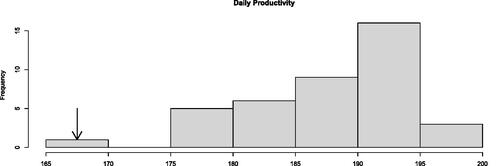
  The histogram in Figure 1 is the simulated daily production attained by a system, where each value in the histogram is the daily production from an independent replication. Clearly there is variability from day to day. One could accept that variability as an inherent feature of the system, but it is also an IE’s obligation to ask why bad days happen because maybe something can be done about it. Obviously, there are no clues in a summary report like a histogram, but there certainly are clues in the complete sample path of the indicated replication—meaning the details of what happened on that bad simulated day—compared to the others.

Figure 1. Histogram of daily productivity values from multiple replications with one particularly bad replication indicated.

Most modern simulation languages will generate a trace, which is a time-stamped record of at least part of what happened at event times; call this a sample path of the system state. Such a record, even from multiple replications of multiple system instances, is at worst “medium data” compared with the “big data” that is routinely the subject of analytics today. Further, the data are clean, well structured and without missing values; they are begging to be investigated. The term simulation analytics (Nelson, 2016) refers to using the simulation-generated data beyond summary statistics for deeper analysis and to answer questions like those posed above.

Several commercial simulation languages provide hooks for, or even include, ML methods such as neural networks. However, simulation data can differ in important ways from the transactional data that are often the focus of data analytics (e.g., purchase decisions along with a vector of customer-specific covariates). For example, a trace is typically a series of time-ordered, dependent values that cannot be treated as independent (feature, label) instances. This opens opportunities for simulation research; here is an example.

Recall that the full system state, as represented conceptually by NSET/QSET, is all of the information that there is to predict the future evolution of the simulation. Some of that state information would also be observable in the real-world system; e.g., queue lengths. As a thought-experiment, imagine creating a database of simulation traces. Then when a state is observed in the real world (e.g., queue lengths), the most similar state observations in the database could be used to predict the future for the real system it simulates. The simplest predictor is kNN, that is the k nearest state vectors in the database to the real-world state.

Of course “nearest” requires a measure of distance. The field of Distance Metric Learning (DML) uses data to train a metric that is more effective than Euclidean distance for kNN and other ML methods (Bellet et al., 2013; Kulis, 2013; Li and Tian, 2018). One formulation of DML is to find an effective matrix $\mathbf{M}$ for the Mahalanobis metric $$d^2({\mathit{s}}_i,{\mathit{s}}_j)={({\mathit{s}}_i-{\mathit{s}}_j)}^{\top }\mathit{M}({\mathit{s}}_i-{\mathit{s}}_j)$$ where in the present context s_i and s_j are two vectors of simulation state values. Notice that squared Euclidean distance is a special case when $\mathbf{M}$ is the identity matrix.

Laidler et al. (2023) considered metric learning for queueing systems, with the specific example of a semiconductor wafer fab where the goal is to classify whether a job released to the fab will be early or late based on observable features such as queue lengths at stations. Using a simulation of the fab, a database of state instances at job release and their ultimate timeliness were generated. Then when a wafer is released to the real fab, the k nearest systems states in the database to the current system state of the fab are used to predict whether the job will be on time or late using kNN and a well-trained distance metric.

Metric learning has been studied extensively, but for situations quite different from the simulation context: The covariate features are typically treated as continuous-valued, rather than being discrete like queue lengths. Further, there is assumed to be a true classification, so that any noise is a type of corruption rather than an inherent part of a stochastic system. And finally, some system states may repeat frequently in the simulation, but DML implicitly assumes unique features for training. All of these differences hinder or completely thwart existing methods for learning $\mathbf{M}.$ This provided an opening for Laidler et al. (2023) to create Stochastic Neighborhood Components Analysis (SNCA), metric learning that not only allows, but exploits these features of simulation data.

There are many such opportunities for simulation analytics. Therefore, a new Book of Output should emphasize post-experiment examination of everything, rather than averages that mask time-dependent effects and discard contextual information. This view will also have implications for Big Consequences in Section 5.

The box score is but a summary; the insight is in the replay.

—The New Book of Output

3. Big computing

“Anyone working on simulation modeling & methods who is not thinking about how it will parallelize is missing the point.”

—B. L. Nelson (2020), in “Statements That Are Sure to Get Me in Trouble”

Since at least the 1970s, the simulation community has been seriously flirting with parallel and distributed simulation; see Fujimoto et al. (2017). “Parallel” is a word like “simulation” that can mean different things to different users. For instance, breaking the simulation model itself into logical pieces that can execute in parallel with occassional coordination is sometimes essential and there have been notable successes; see for examples Perumalla and Seal (2012) and Perumalla et al. (2014).

Far easier, however, is parallelizing the simulation of distinct model instances or replications of a single model instance, and that is the approach discussed here. A common case is obtaining $n\gg 1$ independent replications of $k\ge 1$ model instances by exploiting $p\ll \mathrm{\text{max}}\{k,n\}$ parallel processors. The $\gg$ and $\ll$ indicate that the most substantial computational speed up occurs when many more replications or systems are simulated than there are parallel processors because there is computational overhead to be amortized.

In many programming languages (e.g., Python) parallelizing operations that can be represented as loops is trivially easy,⁴ making looping over $k>1$ models or n replications attractive. More and more commercial simulation software does this automatically on laptop and desktop computers. Distributing simulations across a computing cloud or cluster takes more sophistication, but is certainly doable and will become easier, and it can make computationally infeasible simulations feasible. The differences in parallel architectures will not be discussed here, but they do very much matter.

So why not always parallelize? Consider simulating k = 1 system instance when the number of replications n is not fixed, but instead is the result of achieving some statistical objective, like an estimated relative error of the sample mean of some output being $<5\%.$ This implies that the simulation output values determine when sufficient replications have been achieved.

As far back the 1980s, Phil Heidelberger and Peter Glynn (Heidelberger, 1988; Glynn and Heidelberger, 1991) noted that caution is required in such a case because the order in which requests for replications are distributed to the parallel processors is not necessarily the order in which they are realized (completed and recorded), and this can introduce bias. For instance, suppose we have p = 100 parallel processors, we unleash requests for one replication from each, and we compute the relative error as each output completes. This first 100 will finish, and therefore enter the statistical estimate, in some order. If, for instance, the execution time of a replication is postively correlated with the simulation-generated output’s value, then replications with small output values will tend to be completed first. Statistically, they are not identically distributed.

To convince yourself that this can happen, consider a queueing simulation with a stochastic arrival process for which a replication is 12 simulated hours. Some replications, by chance, see a larger-than-average number of arrivals, which leads to larger-than-average congestion; such a replication can be expected to execute more slowly because more arrivals and service times have to be generated, more events have to be added to and removed from the event calendar, and more waiting-time outputs recorded. Thus completion time is correlated with value. Waiting until the first 100 replications complete before calculating the relative error and distributing any more replication requests solves the statistical probem, but at the cost of idling 99 parallel processors while waiting for the last replication from each batch to complete; a big hit on the speed up.

Unfortunately, Luo et al. (2015) showed that the problem becomes statistically more complicated when multiple model instances are involved (k > 1), such as in parallel simulation optimization. In brief, thoughtlessly parallelizing replications or instances can induce unwanted statistical problems, whereas simple fixes to those problems can seriously degrade the parallel speed up.

Nevertheless, parallel computing greatly extends the limits of problems that can be addressed by simulation, which is good, but clearly parallel simulation requires a different kind of thinking when it comes to analysis methodology. In a single-processor environment, “computationally efficient” almost always means “observation efficient,” that is, obtaining the desired result or inference with as little simulation (e.g., replications) as possible. Computationally efficient parallel simulation is measured in wall-clock time to reach a conclusion, or if parallel capacity is rented, then rental cost. A computationally efficient approach for a single processor can be inefficient in parallel, and vice versa.

To illustrate why different thinking is needed, consider simulation optimization via Ranking & Selection (R&S); see Hong et al. (2021) for a survey of R&S, and for R&S in parallel see Hunter and Nelson (2017). R&S is, in a sense, brute-force optimization because every feasible solution will be simulated. However, R&S is the most well-studied method in simulation, and the only class of methods that provide global optimality guarantees without strong assumptions. Because big computing has pushed back the R&S limit, R&S can be the method of choice even when the decision variable $\mathbf{x}$ has spatial structure.

The canonical R&S problem is to find the best (optimal) among $k\ge 2$ system instances based on the expected value (mean) of some output performance measure such as throughput, profit or utilization. R&S treats the system instances as categorical, so let $x\in \{1,2,\dots ,k\}.$ Further let Y(x) be the random performance output of system design x, with expected value $\mu (x)=\mathrm{E}[Y(x)]$ so the (unknown) best system is $x^{\star }={\text{argmax}}_{x=1,2,\dots ,k}\mu (x).$ For simplicity here assume the best is unique. Finally, let $\widehat{x}$ denote the system ultimately selected by R&S, which will depend on simulation-generated replications $\{Y_j(x),x=1,2,\dots ,k,j=1,2,\dots \}.$ Because the problem is stochastic, a 100% guarantee that $\widehat{x}=x^{\star }$ is not possible but some statistical assurance is desired, and that is what R&S procedures deliver.

R&S—which was initally created for biostatistics problems but has found its greatest application in simulation—was created from the mindset that (a) data (replications in simulation) are expensive (time-consuming in simulation); (b) k is relatively small (say, 5 to 100 system designs); and (c) successfully choosing the best or near-best solution is very important. When R&S was adapted to simulation it was further assumed that the procedure would be executed on a single processor, implying that only one simulation replication or numerical calculation could be completed at a time. The implications of this perspective were profound, and led to R&S procedures doing some or all of the following:

• (a) Carefully allocating one replication at a time, because they are so expensive.

• (b) Eliminating systems using pairwise comparisons because they are powerful discriminators, especially when enhanced with common random numbers (Nelson and Pei, 2021).

• (c) Terminating with strong guarantees, such as the Probability of Correctly Selecting $x^{\star }$ ($\text{PCS}$) being very high, say $\text{PCS}$ near one, or attaining a $\text{PCS}$ that is as large as possible given a budget of simulation effort.

These philosophies led to creative procedures that are amazingly observation or replication efficient. Unfortunately, they do not scale well to a very large number of systems k and $p\gg 1$ parallel processors. To illustrate how parallelizing changes thinking dramatically, the example below shows how a good idea and a horrible idea on a single processor with modest k, become a horrible idea and a good idea, respectively, in parallel with large k.

When k is relatively small and there is p = 1 processor, many observation-efficient R&S procedures are built on sequentially tracking the sum of pairwise differences among systems, with one member of the pair being eliminated if the sum drifts far enough from zero. Specifically, the procedures track ${\sum }_{j=1}^{?}(Y_j(x)-Y_j(x\prime )),\forall x\ne x\prime$ and eliminates one of the pair if it departs from a continuation region, as illustrated in the top plot in Figure 2. This approach allows good systems to eliminate bad ones quickly, and because the replications are paired, it can make effective use of the common random numbers to reduce the variance of the difference, which narrows the region. By setting the statistical error in each pairwise comparison to be small enough, say $\alpha /(k-1),$ a strong family-wise PCS guarantee can be attained. On a single processor this is a good idea that has been widely exploited in practice.

Figure 2. (Top) The sample path of the partial sum ${\sum }_{j=1}^{?}(Y_j(x)-Y_j(x\prime ));$ which system is eliminated depends on the direction the continuation region is exited. The pairwise differences of all surving systems are tracked, and the error for each continuation region controlled at the $\alpha /(k-1)$ level. (Bottom) The sample path of the partial sum ${\sum }_{j=1}^{?}(Y_j(x)-{\overline{\overline{Y}}}_{\text{survivors}});$ the system is eliminated if the boundary of the continuation region is crossed, which may never happen. All surviving systems are tracked, and the error for each continuation region controlled at the α level.

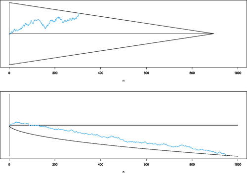
On the other hand, a different partial sum that could be tracked is ${\sum }_{j=1}^{?}(Y_j(x)-{\overline{\overline{Y}}}_{\text{survivors}}),\forall x$ where ${\overline{\overline{Y}}}_{\text{survivors}}$ is the sample average of all observations from all surviving (not-yet-eliminated) systems. In this case a system is eliminated if the sum crosses a one-sided boundary, as illustrated in the bottom plot of Figure 2. When there are only k = 2 systems this partial sum takes four times more observations on average relative to a pairwise difference to eliminate the inferior system. Common random numbers do not help. And finally, the statistical guarantee is on the Expected False Elimination Rate (EFER), the marginal probability that a good system is eliminated, which is not a family-wise guarantee. A horrible idea.

Now suppose that k is huge—maybe thousands to millions—but you have access to $p\gg 1$ parallel processors. Now ${\sum }_{j=1}^{?}(Y_j(x)-Y_j(x\prime )),\forall x\ne x\prime$ is a horrible idea: The $({}_2^k)$ pairwise comparisons explodes into crippling overhead. And since the algorithm has to wait until an observation from each survivor is obtained—a highly coupled operation—processors are frequently idle. And finally, obtaining a family-wise PCS guarantee becomes absurdly demanding due to the curse of multiplicity; this shows up as a much wider, longer continuation region than the one in Figure 2 (top).

On the other hand, ${\sum }_{j=1}^{?}(Y_j(x)-{\overline{\overline{Y}}}_{\text{survivors}}),\forall x$ is a good idea: The number of comparisons is linear in k, the update of ${\overline{\overline{Y}}}_{\text{survivors}}$ is O(1), there is no need to wait for coupling, and the EFER guarantee is scale free, meaning that the boundary in Figure 2 (bottom) does not depend on k. For a deeper discussion of these issues, see Pei et al. (2020, 2022). The key point is that learning to think in parallel requires a reboot that includes a sensitivity to computational as well as statistical efficiency. A statistically efficient simulation-optimization procedure that does not parallelize may be of little value in the future. An additional compelling illustration of thinking differently in parallel for R&S is the knock-out tournament approach described in Zhong and Hong (2022).

Parallel simulation touches many analysis problems, in addition to optimization:

• A consuming research topic for decades was the conundrum of whether to use one long replication vs. multiple independent replications for estimating steady-state (equilibrium) performance measures. The famous paper by Alexopoulos and Goldsman (2004) lays out the issues in a single-processor environment, with one long replication being favored due to the initial-condition-bias problem being difficult to solve. But a one-long-run strategy looks foolish with p > 1 parallel processors available, motivating a reconsideration of the bias-mitigation problem.

• Pseudorandom number generation in a single-processor environment is effectively a solved problem, as there are generators with (for all practical purposes) infinite substreams with infinite periods and good statistical properties; see for instance L’Ecuyer et al. (2002). However, management of pseudorandom numbers in parallel adds additional complexity to ensure that replications that are supposed to be independent have different blocks of pseudorandom numbers; to ensure that replications that are supposed to have common pseudorandom numbers have the same blocks; and to ensure that results are repeatable on different parallel architectures, or even on the same architecture with different loads. See L’Ecuyer et al. (2017).

• Common random numbers approach, which is designed to reduce the variance of differences such as $Y_j(x)-Y_j(x\prime ),$ is most effective when the simulations of model instances can be synchronized (e.g., paired). Synchronization, however, is the enemy of parallel speed up so one has to think carefully as to whether the statistical gain is worth the computational penalty. My conjecture is that typically it will not be worth it.

• I have avoided the issue of which parallel architecture, but it does matter, as well as the number of “processors” p. For instance, Avci et al. (2023) create parallel R&S procedures specifically for desktop/laptop environments with from 8 to 32 processors, $k\le 100$ systems and shared memory, whereas Pei et al. (2022) is tailored for very large numbers of systems and processors in a distributed, message-passing setting; neither would be as effective in the other’s environment

4. Big consequences

“Close enough for government work.”

—Phrase believed to have originated during World War II

Many of society’s most important challenges—healthcare, global terrorism, income inequality, world food supply, power distribution, pandemics—are best modeled as system-of-systems problems. This often means that they cannot be attacked without multiple models, and simulation is often the glue that holds these models together. Saltelli et al. (2020) is a sobering reflection on our profound responsibilities to be careful, open and relevant as model builders for such critical challenges.

Simulation in industrial engineering has traditionally been used for system design, meaning static, one-time decisions such as how many intensive care beds to have in a hospital, how many agents to staff for each hour of the day in a contact center, what layout of machines to deploy in a wafer fab, and so on. However, there are important decisions that are needed in real or near-real time that simulation could support if results are useful and timely. One compelling example is when the simulation is a digital twin and is used to make state-dependent decisions, say if something goes wrong in the real system that it mirrors (Biller et al., 2022). When supporting frequent decisions, small mistakes pile up.

Both societal challenges and real-time decision making put a lot of pressure on the simulation to get it right, but what does that mean? Any discussion of “get it right” raises the issue of model validation. There is a rich, deep and useful history of validation research and methods in systems simulation; see Sargent and Balci (2017). Some of these validation tools address good modeling practices, whereas others are more quantitative.

Everyone wants a valid model, but “valid model” is a difficult concept. If we start from the premise that the simulation and the real or conceptual system it represents are never identical twins, then practical validation boils down to certifying that it is valid enough. This seems difficult to establish, and perhaps more importantly, “valid enough?” begs the question of what to do if the answer is “no” or “unsure.”

Uncertainty Quantification (UQ) is a different take on the validation conundrum. UQ means estimating or bounding the error between the simulation model and real world where it matters, which is in the predicted performance and supported decision. A thorough UQ establishes how much model risk one should hedge against in deploying a simulation-based decision. “Hedging” can mean rolling out a new initiative slowly because the UQ indicates a possibility of trouble; or dedicating extra resources until something like the actual performance predicted by the simulation is observed; or avoiding a change altogether if the model resolution is just not sufficient to ensure averting a disaster. UQ is more actionable than a valid-or-not dichotomy, and an obligation when there are big consequences. This is the main message of the section.

Shortly after the COVID pandemic began in 2020, Professors Peter Frazier, Shane Henderson and David Shmoys along with an army of Ph.D. students in the School of ORIE at Cornell University undertook extensive simulation analysis that was fundamental to Cornell’s decision about whether and how to reopen in fall 2020. To feel good about how relevant simulation can be to decision makers, see Cornell President Pollock’s August 5, 2020 reactivation message at https://covid.cornell.edu/updates/20200805-reactivation-decision.cfm

Although the modeling and simulation behind Cornell’s decision to reopen is interesting, when you dig into the reports you find a full and amazingly candid assessment of the sources and impact of model risk, including parameter uncertainty, model misspecification and offsetting approximations, along with extensive sensitivity analysis, threshold analysis, and estimation of relative instead of absolute differences. One suspects that this candid and quantitative risk analysis gave decision makers more confidence about what to do, where to be careful, and what key indicators to track. This is an example of simulation being central to both a system-of-systems problem, and being used for frequent adjustments as new information was realized.

For simulation to be ready for big consequences, a change in simulation’s treatment of risk is needed, along with the research to support it. Two related issues stand out: Dispensing with an overreliance on averages and Confidence Intervals (CIs) to quantify system performance, and disentangling estimation risk and model risk and reality risk.

Averages and CIs, a key tactical problem from Conway (1963), convey no information about how predictable system performance is, which is often more important than the long-run average. For an intuitive simulation output plot that captures both aspects see Nelson (2008). More generally, default simulation input and output displays that emphasize their distributions and relationships would give users a better understanding of system behavior. Section 3.2 described going into the simulation sample path for deeper information, including establishing relationships and the distribution of performance. Here I focus on the various types of UQ this might support.

Let $\mathbf{x}$ be a decision that can be implemented in the real world and also in the simulation of it. For instance, in the air traffic disruption recovery problem of Rhodes-Leader et al. (2022), $\mathbf{x}$ specified the recovery decision for each affected flight. Further, let $Y^R(\mathbf{x})$ be the real-world response to decision $\mathbf{x}$ with (unknown) mean ${\mu }^R(\mathbf{x})=\mathrm{E}[Y^R(\mathbf{x})];$ this was the cost of recovery in Rhodes-Leader et al. (2022), and the $\mathbf{x}$ that minimized this expectation was the desired action. From the simulation, let $Y_j^S(\mathbf{x}),j=1,2,\dots ,n$ be the simulation response from n i.i.d. replications with (also unknown) mean ${\mu }^S(\mathbf{x})=\mathrm{E}[Y^S(\mathbf{x})],$ and let ${\overline{Y}}^S(\mathbf{x})$ be the sample mean of those replications. All of the following risks are relevant:

• Estimation risk refers to the fact that ${\overline{Y}}^S(\mathbf{x})\ne {\mu }^S(\mathbf{x})$—the simulation sample mean does not equal its expected value—and this risk is often captured by a CI. Every simulation language reports these and there is a big emphasis on obtaining statistically valid CIs.

• Model risk refers to the fact that, among other things, ${\mu }^S(\mathbf{x})\ne {\mu }^R(\mathbf{x});$ that is, there is a potential mismatch between the mean of the simulation and the mean of real-world performance (and more generally their distributions). Models are not perfect.

• Reality risk refers to the fact that, among other things, $Y^R(\mathbf{x})\ne {\mu }^R(\mathbf{x})$ in general; that is, the real world itself is variable, so even if the simulation provided the optimal decision $\mathbf{x}$ in terms of mean performace, chances are that what actually happens will not be the mean, and in fact might be better or worse.

Reality risk is quantified to some extent by looking beyond the mean or average performance from the simulation, but unless the same decision $\mathbf{x}$ is employed repeatedly in the same real-world setting, it is hard to know whether unexpected results are due to reality risk or a misalignment between the simulation and real world (model risk). Accounting for reality risk is a huge and important challenge when simulation is employed repeatedly for context-sensitive decisions. See Rhodes-Leader and Nelson (2023) for some ideas about assessing digital-twin and real-world misalignment in the presence of reality risk.

Recently there has been considerable UQ success in assessing or hedging against model risk due to input models that are estimated from data. The term used for this risk in simulation is input uncertainty. Loosely, “assessing” means quantifying the additional error between the simulation and real world, for instance via an inflated CI that accounts for both estimation and input-uncertainty error. “Hedging,” on the other hand, tries to identify the worst case input models within a space of plausible input models. Input uncertainty is a topic on which research has been advancing rapidly, but a relatively recent survey is Barton et al. (2022). Notice that pushing more of the simulation model into being an input—as described in Section 3.1—allows more of the model risk to be treated as input uncertainty.

The most basic UQ tool for model risk is sensitivity analysis, which can be global (across the full range of possible changes) and local (small changes from a nominal model). Unfortunately, sensitivity analysis does not play as large a role in simulation as it does in mathematical optimization or stochastic processes; it should. In the related field of computer experiments—essentially deterministic simulations—sensitivity analysis with respect to model parameters about which there might be some uncertainty, or that might be changed to yield improved or robust performance, is well developed; see for instance Saltelli et al. (2008).

For systems simulation sensitivity analysis it is easy to forget that classic experiment design is a well-developed and powerful tool—particularly for global sensitivity—when one can afford simulations at various settings of possibly sensitive factors. See Sanchez et al. (2020) for a gentle introduction with lots of references. Unfortunately, our infatuation with ML has pushed experiment design into the background.

Local sensitivity analysis can be a bit more subtle with some of what appears in current software being hard to interpret or even misleading. Here is an illustration of why meaningful sensitivity analysis is difficult: In Factory Physics (Hopp and Spearman, 2011), the authors coined the phrase “the corrupting influence of variability” in describing the physics of manufacturing systems. Variability matters. So a natural sensitivity question to ask of, say, your wafer fab simulation is, “How sensitive is my mean cycle time to the variance of the developer step?” Great question, until you try to decide what it means.

Let Z be the input random variable representing time to complete the developer step and let Y be the output random variable representing the average cycle time. What one wants is something like $\partial \mathrm{E}(Y)/\partial \text{Var}(Z)$ that is meaningful and estimable. However, unless it is the case that $Z=\mu +\sigma W,$ where W has mean 0 and variance 1, there are lots of ways that changes in $\text{Var}(Z)$ can affect Z. Which one is relevant?

When Z has a parametric input distribution with natural parameter θ, partial derivatives with respect to components of θ can be estimated (see for instance Fu (2006)). However, for something like a gamma distribution whose natural parameters are shape and scale, $\theta =(\alpha ,\beta ),$ partial derivatives of the output mean (or other properties) with respect to these parameters do not answer the sensitivity-with-respect-to-variance question. Recall that ${\sigma }^2=\alpha /{\beta }^2$ for the gamma distribution.

As one solution Jiang et al. (2021) suggested using meaningful directional derivatives with respect to θ: $$\frac{\partial \mathrm{E}(Y)}{\partial \text{Var}{(X)}_{\mathit{d}}}=\frac{{\mathit{d}}^{\top }{\nabla }_{\theta }\mathrm{E}(Y)}{{\mathit{d}}^{\top }{\nabla }_{\theta }\text{Var}(X)}$$ where $\mathbf{d}$ is a direction vector and $\nabla$ is the gradient operator. The ${\nabla }_{\theta }\text{Var}(X)$ is computable (at least numerically) for any parameteric distribution, and as mentioned above ${\nabla }_{\theta }\mathrm{E}(Y)$ is estimable using now standard simulation methods. Meaningful directions $\mathbf{d}$ include steepest ascent, minimum mean change, or something application specific. Steepest ascent implies that within this parametric family θ changes so that the variance increases as fast as possible; this might represent a worst-case scenario when variance is bad. Minimum mean change implies that the parameter θ changes to increase the variance without changing the mean developer time; this is likely what many users want. An application-specific direction comes from some particular knowledge of how increased variance might change the developer step. And this meaningful-direction approach is not restricted to sensitivities of means with respect to variance.

As an illustration of why a careful definition of sensitivity is important, Jiang et al. (2021) demonstrated in their wafer fab example that 27 hrs/hr² is the steepest-ascent sensitivity of mean cycle time to variance, while 0.3 hrs/hr² is the minimum-mean-change sensitivity to variance, a huge difference indicating dramatially different levels of variance risk. Routine and interpretable sensitivity analysis is the very least that should accompany any simulation of consequence, but more research is needed to make it so.

Returning to repeated, context-sensitive decisions, two interesting paradigms have arisen for leveraging simulation: online simulation as needed, and offline simulation for online application. To date the digital twin setting has emphasized online simulation. In Rhodes-Leader et al. (2022) the digital twin represents airspace in the UK. When a disruption occurs due to weather or aircraft breakdown the ideal is to undertake a simulation optimization in real time to decide what flights to delay, reroute or cancel. However, given the complexity of an airspace model and the state of the art in simulation optimization, online simulation optimization is computationally impossible for this application. Therefore, to facilite real-time decisions, mathematical programming is used to generate a small number of good schedules, and then simulation optimization is used to fine-tune them and select the best. Digital twins are a challenging domain for simulation methodology that forces consideration of simulation use time vs. real-world decision time. In any event it is certainly a good application for the strategic use of parallel simulation.

Offline simulation for online application, on the other hand, means doing all or nearly all simulation that will be needed to support decision making in advance of when decisions have to be made. For example, Shen et al. (2021) consider R&S when the best system/decision depends on contemporaneous covariate information, such as an arriving patient’s health record. A carefully designed offline simulation experiment that covers the space of possible covariate values then provides a metamodel to be queried for the best decision whenever actual covariate values are realized, while still providing a strong statistical guarantee of optimality. Databases of simulation results can be queried much more rapidly than large-scale simulation experiments can be conducted, making offline simulation for online application a very promising direction.

That said, simulation optimization is not immune to model and reality risk. SO considers problems of the form ${\mathrm{\text{max}}}_{\mathbf{x}\in \mathcal{X}}\mathrm{E}[Y(\mathbf{x})],$ with methods tailored to what is known about the simulation and about $\mathbf{x}.$ At noted earlier, R&S is one class of SO methods. The reality of model risk is that the simulation model may not have sufficient resolution to distinguish which simulated solution is the real-world optimal solution if model risk is considered. Song and Nelson (2019) show that it is sometimes easier to determine the optimal solution than to estimate the actual real-world performance in the presence of input uncertainty when that uncertainty affects all the feasible solutions near the optimal similarly. This is an interesting direction, but barely explored. A different approach is to find a defensive optimal solution, such as one that optimizes over the worst-case performance for plausible input models; see for instance Fan et al. (2020). The trick is to avoid being overly conservative.

Claiming optimality in the presence of significant model risk is misleading, and a thorough UQ should accompany any recommended solution. This is yet another challenge posed by big consequences.

5. Conclusion

The premise of this article is that big data—both the ability to collect it and the tools to analyze it—big computing—cheap and readily available parallel processing capability—and big consequences—from society’s necessary reliance on model-based decisions—should be pushing computer simulation for industrial engineering in directions that could not have been anticipated in the formative year of 1963. Both research and practice tend to develop momentum that carry them in an initial direction until some outside forces alter it; my claim is that these are such forces. The good news for simulation is that these forces are not only compatible with, but in fact enhance the power of, computer simulation.

Acknowledgments

The author thanks Eunhye Song and two referees for helpful comments and insight.

Additional information

Funding

This work was partially supported by National Science Foundation Grant No. CMMI-2206973. Division of Civil, Mechanical and Manufacturing Innovation.

Notes on contributors

Barry L. Nelson

Barry L. Nelson is the Walter P. Murphy Professor Emeritus of the Department of Industrial Engineering and Management Sciences at Northwestern. His research focus is the design and analysis of computer simulation experiments on models of discrete-event, stochastic systems, including methodology for simulation optimization, quantifying and reducing model risk, variance reduction, output analysis, metamodeling and multivariate input modeling. He has published numerous papers and three books, including Foundations and Methods of Stochastic Simulation: A First Course (second edition, Springer, 2021). Nelson is a Fellow of INFORMS and IISE. Further information can be found at http://users.iems.northwestern.edu/∼nelsonb/.

Notes

1 A GSMP is a stochastic process description of a discrete-event simulation that is suitable for proving structural results; see for instance Whitt (1980).

2 Conway (1963) was a refinement of Conway et al. (1959)

3 To the best of my knowledge this did not happen at Sloan, which kind of proves the point.

4 This may be a slight exaggeration, because care may be needed to ensure that each replication uses different pseudorandom numbers, as discussed later in this section.

References

- Alexopoulos, C. and Goldsman, D. (2004) To batch or not to batch? ACM Transactions on Modeling and Computer Simulation, 14(1), 76–114.
- Avci, H., Nelson, B.L., Song, E. and Wächter, A. (2023) Using cache or credit for parallel ranking and selection. ACM Transactions on Modeling and Computer Simulation. Forthcoming.
- Barton, R.R., Lam, H. and Song, E. (2022) Input uncertainty in stochastic simulation, in The Palgrave Handbook of Operations Research, Springer, New York, pp. 573–620.
- Bellet, A., Habrard, A. and Sebban, M. (2013) A survey on metric learning for feature vectors and structured data. arXiv preprint arXiv:1306.6709.
- Biller, B., Jiang, X., Yi, J., Venditti, P. and Biller, S. (2022) Simulation: The critical technology in digital twin development, in Proceedings of the 2022 Winter Simulation Conference, IEEE Press, Piscataway, NJ, pp. 1340–1355.
- Conway, R.W. (1963) Some tactical problems in digital simulation. Management Science, 10(1), 47–61.
- Conway, R.W., Johnson, B.M. and Maxwell, W.L. (1959) Some problems of digital systems simulation. Management Science, 6(1), 92–110.
- Fan, W., Hong, L.J. and Zhang, X. (2020) Distributionally robust selection of the best. Management Science, 66(1), 190–208.
- Fu, M.C. (2006) Gradient estimation, in Handbooks in Operations Research and Management Science, volume 13, Elsevier, Amsterdam, pp. 575–616.
- Fu, M.C. (2015) Handbook of Simulation Optimization. Springer, New York.
- Fujimoto, R.M., Bagrodia, R., Bryant, R.E., Chandy, K.M., Jefferson, D., Misra, J., Nicol, D. and Unger, B. (2017) Parallel discrete event simulation: The making of a field, in Proceedings of the 2017 Winter Simulation Conference, IEEE Press, Piscataway, NJ, pp. 262–291.
- Glynn, P.W. and Heidelberger, P. (1991) Analysis of parallel replicated simulations under a completion time constraint. ACM Transactions on Modeling and Computer Simulation, 1(1), 3–23.
- Heidelberger, P. (1988) Discrete event simulations and parallel processing: Statistical properties. SIAM Journal on Scientific and Statistical Computing, 9(6), 1114–1132.
- Hong, L.J., Fan, W. and Luo, J. (2021) Review on ranking and selection: A new perspective. Frontiers of Engineering Management, 8(3), 321–343.
- Hopp, W.J. and Spearman, M.L. (2011) Factory Physics. Waveland Press, Long Grove, IL.
- Huang, Z. and Kumar, A. (2012) A study of quality and accuracy trade-offs in process mining. INFORMS Journal on Computing, 24(2), 311–327.
- Hunter, S.R. and Nelson, B.L. (2017) Parallel ranking and selection. In Advances in Modeling and Simulation: Seminal Research from 50 Years of Winter Simulation Conferences, Springer, New York, pp. 249–275.
- Jiang, W.X. and Nelson, B.L. (2018) Better input modeling via model averaging, in Proceedings of the 2018 Winter Simulation Conference, IEEE Press, Piscataway, NJ, pp. 1575–1586.
- Jiang, X., Nelson, B.L. and Jeff Hong, L. (2021) Meaningful sensitivities: A new family of simulation sensitivity measures. IISE Transactions, 54(2), 122–133.
- Kulis, B. (2013) Metric learning: A survey. Foundations and Trends® in Machine Learning, 5(4), 287–364.
- Laidler, G., Morgan, L., Nelson, B.L. and Pavlidis, N. (2023) Stochastic neighbourhood components analysis. Under review.
- L’Ecuyer, P., Munger, D., Oreshkin, B. and Simard, R. (2017) Random numbers for parallel computers: Requirements and methods, with emphasis on GPUs. Mathematics and Computers in Simulation, 125, 3–17.
- L’Ecuyer, P., Simard, R., Chen, E.J. and Kelton, W.D. (2002) An object-oriented random-number package with many long streams and substreams. Operations Research, 50(6), 1073–1075.
- Li, D. and Tian, Y. (2018) Survey and experimental study on metric learning methods. Neural Networks, 105, 447–462.
- Luo, J., Hong, L.J., Nelson, B.L. and Wu, Y. (2015) Fully sequential procedures for large-scale ranking-and-selection problems in parallel computing environments. Operations Research, 63(5), 1177–1194.
- Nance, R.E. and Overstreet, C.M. (2017) History of computer simulation software: An initial perspective, in Proceedings of the 2017 Winter Simulation Conference, IEEE Press, Piscataway, NJ, pp. 243–261.
- Nelson, B.L. (2004) 50th anniversary article: Stochastic simulation research in Management Science. Management Science, 50(7), 855–868.
- Nelson, B.L. (2008) The MORE plot: Displaying measures of risk & error from simulation output, in Proceedings of the 2008 Winter Simulation Conference, IEEE Press, Piscataway, NJ, pp. 413–416.
- Nelson, B.L. (2016) Some tactical problems in digital simulation for the next 10 years. Journal of Simulation, 10(1), 2–11.
- Nelson, B.L. and Pei, L. (2021) Foundations and Methods of Stochastic Simulation. Springer, New York.
- Nelson, B.L., Wan, A.T., Zou, G., Zhang, X. and Jiang, X. (2021) Reducing simulation input-model risk via input model averaging. INFORMS Journal on Computing, 33(2), 672–684.
- Pei, L., Nelson, B.L. and Hunter, S.R. (2020) Evaluation of bi-PASS for parallel simulation optimization, in Proceedings of the 2020 Winter Simulation Conference, IEEE Press, Piscataway, NJ, pp. 2960–2971.
- Pei, L., Nelson, B.L. and Hunter, S.R. (2022) Parallel adaptive survivor selection. Operations Research. https://doi.org/10.1287/opre.2022.2343
- Perumalla, K.S., Park, A.J. and Tipparaju, V. (2014) Discrete event execution with one-sided and two-sided gvt algorithms on 216,000 processor cores. ACM Transactions on Modeling and Computer Simulation, 24(3), 1–25.
- Perumalla, K.S. and Seal, S.K. (2012) Discrete event modeling and massively parallel execution of epidemic outbreak phenomena. Simulation, 88(7), 768–783.
- Rhodes-Leader, L., Nelson, B., Onggo, B.S. and Worthington, D. (2022) A multi-fidelity modelling approach for airline disruption management using simulation. Journal of the Operational Research Society, 73(10), 2228–2241.
- Rhodes-Leader, L. and Nelson, B.L. (2023) Tracking and detecting systematic errors in digital twins, in Proceedings of the 2023 Winter Simulation Conference. IEEE Press, Piscataway, NJ (in press).
- Saltelli, A., Bammer, G., Bruno, I., Charters, E., Fiore, M.D., Didier, E., Espeland, W.N., Kay, J., Piano, S.L., Mayo, D., Pielke, R., Portaluri, T., Porter, T.M., Puy, A., Rafols, I., Ravetz, J.R., Reinert, E., Sarewitz, D., Stark, P.B., Stirling, A., van der Sluijs, J., and Vineis, P. (2020) Five ways to ensure that models serve society: A manifesto. https://www.nature.com/articles/d41586-020-01812-9. Accessed 2023-08-02.
- Saltelli, A., Ratto, M., Andres, T., Campolongo, F., Cariboni, J., Gatelli, D., Saisana, M., and Tarantola, S. (2008) Global Sensitivity Analysis: The Primer. John Wiley & Sons, New York.
- Sanchez, S.M., Sanchez, P.J. and Wan, H. (2020) Work smarter, not harder: A tutorial on designing and conducting simulation experiments, in Proceedings of the 2020 Winter Simulation Conference, IEEE Press, Piscataway, NJ, pp. 1128–1142.
- Sargent, R.G. and Balci, O. (2017) History of verification and validation of simulation models, in Proceedings of the 2017 Winter Simulation Conference, IEEE Press, Piscataway, NJ, pp. 292–307.
- Shen, H., Hong, L.J. and Zhang, X. (2021) Ranking and selection with covariates for personalized decision making. INFORMS Journal on Computing, 33(4), 1500–1519.
- Song, E. and Nelson, B.L. (2019) Input–output uncertainty comparisons for discrete optimization via simulation. Operations Research, 67(2), 562–576.
- Tocher, K. (1963) The Art of Simulation. The English Universities Press, London.
- Whitt, W. (1980) Continuity of generalized semi-Markov processes. Mathematics of Operations Research, 5(4), 494–501.
- Zhong, Y. and Hong, L.J. (2022) Knockout-tournament procedures for large-scale ranking and selection in parallel computing environments. Operations Research, 70(1), 432–453.
- Zhu, T., Liu, H. and Zheng, Z. (2023) Learning to simulate sequentially generated data via neural networks and Wasserstein training. ACM Transactions on Modeling and Computer Simulation, 33(9), 1–34.