Intra-annual variations of vegetation status in a sub-tropical deciduous forest-dominated area using geospatial approach: a case study of Sali watershed, Bankura, West Bengal, India

ABSTRACT

Intra-annual dynamics of vegetation status is very important to understand the spatial ecological environment. In this study, pixel wise temporal variation of vegetation status has been assessed using normalized differential vegetation index (NDVI) from Landsat 8 OLI data of 2014. Month-wise vegetation statuses were employed to understand the status of vegetation dynamics for the Sali River watershed. We have found that vegetation status (VS) of this study area varied with respect to space and time. We have identified two dominant natures of NDVI fluctuation, one with a single peak coming out of Sal forest and another with multiple peaks which is from paddy fields. NDVI curve of natural vegetation follows a rainfall pattern and depicts a single peak during the rainy season with the moderate standard deviation (S.D.) and coefficient of variation (C.V.). On the other hand, the area associated with population pressure and agricultural fields shows multiple peaks as well as a high degree of S.D. and C.V. of NDVI during the months of April, August and December.

KEYWORDS:

• Vegetation dynamics
• normalized differential vegetation index
• Landsat 8 OLI
• remote sensing and GIS
• Sali River watershed

1. Introduction

Human species are about to be acknowledged as the only intelligent and advanced species in this Spaceship Earth, where each species doing their own role to sustain the environment (Pal, Chakrabortty, Malik, & Das, 2018). Spatial distribution of natural vegetation and its quality are a crucial part of our Earth’s life-supporting system and environment for providing basic support for sustaining life on this Earth and achieving sustainable environmental goal. On the other hand, unplanned deforestation issignificantly hampering the human being as well as the lives of other species in a very dangerous manner (UN Report, 2019). Quality of vegetation and its spatial coverage can affect numerous aspect of the environment as well as living beings (Naidoo et al., 2019). In this regard, monitoring and assessing the status of vegetation is one of the significant aspects of environmental health assessment and mitigating global climate change (Alberdi et al., 2019; Bjorkman et al., 2019; UN report on environment, 2019). Apart from this, it also provides valuable information regarding the natural and man-made environments through quantifying vegetation cover from smaller to larger scales at a given point of time or over a continuous period (Xiao, 2004; Xie, Sha, & Yu, 2008) and helps in the protection and restoration programmes of vegetation (Egbert, Park, Price, Lee, & Nellis, 2002; He, Zhang, Li, & Shi., 2005). Above all, Knight, Lunetta, Ediriwickrema and Khorram (2006) argued that strong pretences should be given towards close monitoring of vegetation for the assessment of the environmental system, which is also an urgent need for the society.

Traditional methods of vegetation monitoring (e.g., literature reviews, field surveys, map interpretation and collateral and ancillary data analysis) are time-consuming and not so effective to acquire information and often very much expensive and quite tough to conduct (Xiao, 2004; Xie et al., 2008). In this connection, remote sensing (RS) and geographical information system (GIS) provides a practical and economical means to study vegetation cover and its quality, especially over large spatial and temporal scale (Langley, Cheshire, & Humes, 2001; Nordberg & Evertson, 2005; Sarkar & Kafatos, 2004). Normalized differential vegetation index (NDVI) has been applied in this study to represent vegetation status (VS). Temporal variation of NDVI is strongly associated with changes in the state of surface energy, water balance (Chase, Pielke, Kittel, Nemani, & Running, 1996), carbon cycle (Betts, Beljaars, Miller, & Viterbo, 1996; Eastman, Coughenour, & Pielke, 2001), natural hazards (drought, wind, floods, rain and anthropogenic activity) (Telesca & Lasaponara, 2006; Telesca, Lasaponara, & Lanorte, 2008) and so on. These components are strongly related to the dynamic changes in spatial coverage of vegetation (Telesca & Lasaponara, 2006) and feedback on climate (Eswaran, Lal, & Reich, 2001; Foley, Kutzbach, Coe, & Levis, 1994). So, the annual variation of vegetation study is an important part for the understanding and management of the environment. The inter-annual and inter-seasonal variability of NDVI has been studied by many scholars (Anyamba & Eastman, 1996; Eastman & Fulk, 1993; Guo, Zhang, Yuan, Zhao, & Xue, 2015; Li & Kafatos, 2000; Myneni, Los, & Tucker, 1996; Nemani et al., 2003; Sarkar & Kafatos, 2004). Most of their studies were focused on the factors behind the natural oscillation of natural vegetation. Bjorkman et al. (2019) reviewed the temporal changes in vegetation status in Arctic environments to highlight the demand for further geographically inclusive, combined and comprehensive monitoring efforts that can better resolve the interacting impacts of warming and other local and regional ecological factors, whereas Fu et al. (2018) studied similar kinds of study from climate changes for Qaidam Basin. Yang et al. (2018) evaluated the health situation of Poyang Lake using vegetation-based indices. Demisse et al. (2018) and Nanzad et al. (2019) applied vegetation indices to evaluate the drought conditions.

Sarkar and Kafatos (2004) studied on the Indian subcontinent for several years to study the variability of vegetation and found the dominance of local climate anomaly in determining the vegetation. Several kinds of datasets, e.g., NOAA-AVHRR, SPOT-VGT, MODIS and GIMMS have been used (NOAA-AVHRR, SPOT-VGT, MODIS and GIMMS) to study the variability of vegetation at the local, regional and global scale (de Jong, de Bruin, de Wit, Schaepman, & Dent, 2011; Detsch, Otte, Appelhans, Hemp, & Nauss, 2016; Dubovyk, Landmann, Erasmus, Tewes, & Schellberg, 2015; Fensholt & Proud, 2012; Guo et al., 2015; Hou, Zhang, & Wang, 2011; Jeong, HO, GIM, & Brown, 2011; Lanorte, Lasaponara, Lovallo, & Telesca, 2014; Lu, Kuenzer, Wang, Guo, & Li, 2015; Martínez & Gilabert, 2009; Schucknecht, Erasmi, Niemeyer, & Matschullat, 2013; Sobrino & Julien, 2011; Teferi, Uhlenbrook, & Bewket, 2015; Zhao et al., 2013).

Primary objective of this study is to understand the intra-annual variation of vegetation status over a monsoon-dominated climatic area using NDVI on Landsat 8 dataset. This kind of study will enable us in a more robust identification of changes in vegetation status with greater spatial detail. It would provide us with a unique perspective to understand the spatial–temporal dynamics of vegetation status, which will help us significantly in the monitoring and management of the vegetation status.

2. Database and methodology

2.1 Study area

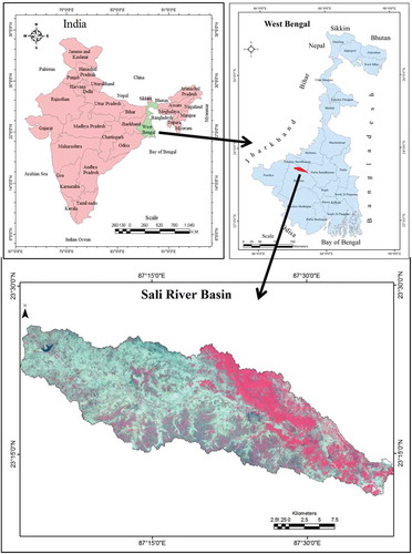
Sali River is a right-bank tributary of the Damodar River within Bankura District (22°38´ to 23°38´ north latitude and 86°36´ to 87°46´ east longitude) of West Bengal, India. According to the watershed atlas of India, Sali River (2A2D4 is the watershed number according to Watershed Atlas of India) can be called as watershed because it has an area within 750 sq. km (Figure 1). This river has originated from a village near Gangajalghati police station of Bankura District. After that, this river crossed Gangajalghati, Barjora, Sonamukhi and Indus P.S. and fall into Damodar River immediately to the north of the Somsar, a village in the Indus. It has a large course of 73.6 km and it drained approximately 714 sq. km of the inter-fluvial parts of Damodar and Dwarkeswar rivers. This river facilitates local irrigation in its neighbouring areas. Cainozoic laterite can be found in its upper part and some Pleistocene middle to upper and Holocene sediment can be found on the lower part (Geological and Mineral Map of West Bengal, Govt. of India, 1999). Climatically, this river watershed belongs to the dry tropical and sub-humid having yearly rainfall of 1480.62 mm. Most of the rainfall occurred during four wet months (June, July, August and September). Maximum and minimum temperature ranges between 45°C and 10°C normally (Indian Meteorological Department) (Table 1). Here, several protected forests can be found such as Beliatore Protected Forest, Sonamukhi Protected Forest, Patsol Protected Forest, Gangabandh Protected Forest, Gangajalghati Protected Forest and so on. Nature of forest type is open mixed jungle, dense mixed jungle mainly Sal (Shorea robusta), fairly dense mixed jungle, dense Sal, open Sal and so on.

Figure 1. Location map of the study area.

2.2 Methods

The study considered the vegetation dynamics using a spectral index of NDVI and statistical investigation has been done to explore the intra-annual vegetation dynamics. In this study, we have used 10 Landsat 8 images from different months of the year of 2014, downloaded from GLOVIS (Table 2). After completing the required atmospheric correction, NDVI has been extracted for the respective time periods. Pixel-wise information about vegetation status has been analysed to understand the temporal vegetation dynamics and its variation has been assessed through using the coefficient of variation (C.V.) and standard deviation (S.D.) of NDVI. Along with this, rainfall pattern has been compared with 2014 vegetation dynamics, which will help us to understand the association between rainfall and vegetation dynamics. A major limitation of this study is that the research work was done using 10 months’ data sets as we have found that the cloud-free data were available only for 10 months (excluding July and September months) for the year of 2014. Beyond that year, the very same cloud-free data were not available at all.

Table 1. Climatic condition of study area.

	Jan	Feb	Mar	Apr	May	Jun	Jul	Aug	Sep	Oct	Nov	Dec
AvgTemp (C)	19.5	22.1	27.4	31.4	31.5	31.1	29	28.9	28.8	27.3	22.9	19.8
Min. Temp (C)	12.7	15.2	20.2	24.4	26.2	26.5	25.8	25.8	25.5	23.1	17	13.2
Max. Temp (C)	26.4	29.1	34.7	38.4	36.8	35.7	32.2	32	32.2	31.5	28.9	26.4
Precipitation (mm)	13	19	21	33	67	179	255	253	227	76	12	2

Table 2. Details of satellite data.

Data Type	Date of Acquisition
Landsat 8	24 January 2014; 24 February 2014; 24 March 2014; 24 April 2014; 24 May 2014; 16 June 2014; 19 August 2014; 22 October 2014; 23 November 2014; 25 December 2014

2.3 Normalized Difference Vegetation Index (NDVI) analysis

NDVI is one of the most frequently used methods for vegetation cover study. It is generally calculated by the ratio between the red and near-infrared band (Bannari, Morin, Bonn, & Huete, 1995; Rouse, Haas, Deering, & Schell, 1974). NDVI is very helpful to sense diverse physical characteristics of vegetation canopy such as leaf area index (Carlson & Ripley, 1997), fractional vegetation cover (Carlson & Ripley, 1997; Guerschman et al., 2009; Jia et al., 2016; Scanlon, Albertson, Caylor, & Williams, 2002; Xiao et al., 2005), vegetation condition (Fensholt, 2004; Telesca et al., 2008) and biomass (Carlson & Ripley, 1997). Pettorelli et al. (2005) used this index to assess the environmental change and its impact. It can provide a useful measure of photosynthetically dynamic biomass (Tucker & Sellers, 1986) land cover variations (Cuomo, Lanfredi, Lasaponara, Macchiato, & Simoniello, 2001; Huemmrich, Black, Jarvis, McCaughey, & Hall, 1999; Lanfredi, Lasaponara, Simoniello, Cuomo, & Macchiato, 2003; Myneni et al., 1996; Telesca & Lasaponara, 2006; Telesca et al., 2008). It is also correlated with rainfall, temperature and evapotranspiration in a broad range of environmental conditions (Cihlar, Laurent, & Dyer, 1991; Gray & Tapley, 1985; Sarkar & Kafatos, 2004).

NDVI has been calculated following Rouse et al. (1974), which is given below

(1) $NDVI=(NIR-RED)/(NIR+RED)$(1)

where RED is the surface reflectance of wavelengths in the visible (λ ~ 0.6 μm) and NIR is the surface reflectance of wavelengths (λ ~ 0.8 μm) of the spectrum, respectively.

Several places were visited for field verifications using the Garmin GPS. In this study, we have collected 91 sample data from eight different places maintaining minimum 100 m distance between two sample points based on accessibility and nature of land use and land cover. Several field visits were done during pre-monsoon, monsoon and post-monsoon seasons of the year to understand the changing nature of vegetation dynamics. Monthly total rainfall data for the months of 2014 were also used to find out the relation between rainfall and vegetation in this area. After collecting all the information about NDVI and its selected field area expression, temporal variation, frequency distribution, simple line graph, C.V. and its S.D. were computed to express the nature of vegetation dynamics.

3. Results and analysis

3.1 Status of vegetation covers in the Sali River

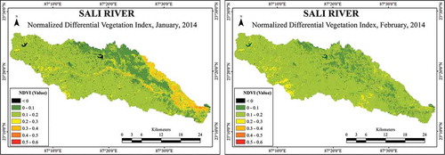
Status of vegetation can be defined by several vegetation indices, but we have relied on the NDVI for understanding the vegetation coverage as well as its quality due to its simplicity, reliability and popularity. In this study, we have calculated the NDVI for different months of 2014. In January 2014, we have found the high degree of NDVI along the Damodar River as well as along the main Sali River (NDVI >0.3). It is may be due to the fact that during this time, river base flow is occurring and with the help of localized irrigation techniques, people used to cultivate vegetables in their land. On the other hand, Sal forest in this area does not represent the high amount rather than they are showing some medium NDVI (0.1–0.3). Maximum portion of this watershed was under low NDVI status (less than 0.2). In the month of January, waterbody showed very low NDVI (less than 0). The average NDVI of January month was 0.147. In case of February, we have found that except few patches most of the area was under low NDVI (less than 0.2) and average NDVI value is relatively lower (0.140) than January (Figure 2). This may be the result of a long dry spell period in this area and devoid of a crop in the field.

Figure 2. NDVI of Sali River for the month of January (left) and February (right).

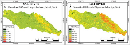
During the month of March, some portion of the watershed area represented a moderate concentration of NDVI and these are nothing but the agricultural field area with the irrigation facilities and these areas during April turned into very high-quality vegetation (NDVI >0.4). Another significant fact was that overall watershed area showed medium NDVI (0.2–0.3). Apart from these concentrated agricultural field areas, forest area up to April continuously showed a relatively low amount of NDVI compared to its surrounding watershed due to the absence of green leaves (Figure 3. left). But after this month of April, the forest cover area started to represent higher NDVI with the knocking of new leaves throughout the forest cover area (Figure 3 (right)).

Figure 3. NDVI of Sali River for the month of March (left) and April (right).

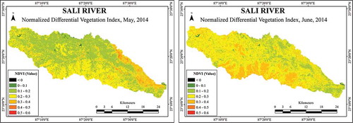
After that, during the month of May, the highest NDVI was recorded along Damodar River (Figure 4 (left)), whereas forest area still represented moderate NDVI (0.2–0.3). From the month of June to October, the highest NDVI can be found over the forest cover area (>0.4). Rest of the parts remains low to moderate. At this stage, small amount of precipitation (67 mm) occurred, which leads to the reactivation of vegetation in this area. Moderate-to-high amount of NDVI can be found over this watershed with the upcoming months of June and monsoon precipitation (179 mm). The highest reflection of NDVI occupied by the forest area, whereas the rest of them reflecting moderate NDVI (Figure 4 (right)).

Figure 4. NDVI of Sali River for the month of May (left) and June (right).

With the passage of time, monsoon precipitation takes over the region, leading to the highest reflectance of NDVI among the all other months of the year. During the month of August (Figure 5. left), the highest amount of NDVI found over the Sal dominated forest area. Agricultural fields were associated with starting of cultivation leading towards the development of low-to-moderate NDVI. During this month, 55% of the watershed area covered with moderate-to-high NDVI (>0.4). Vegetation condition improved during the upcoming months of October (Figure 5 (right)). As a result, about 90% of the area represented moderate-to-high NDVI (0.3–0.4). This may be the result of monsoon precipitation over the watershed area.

Figure 5. NDVI of Sali River for the month of August (left) and October (right).

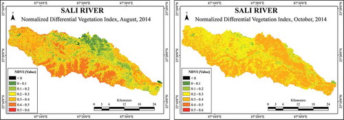
Vegetation status again started to decrease. In the case of November, 74% of the study area comes under a low status of vegetation condition (NDVI 0.2–0.3). Here, during this month, Sal forests remain at the top of the NDVI value compared to its other areas in this watershed (Figure 6 (left)). In the case of December, forest area (60%) still remains high relatively high to its surrounding area (Figure 6 (right)). However, along the Damodar River, 22% area of Sali River represented a higher amount of NDVI (0.3–0.4). This concentration of the higher amount of NDVI may be the result of agricultural activity with the help of local irrigational facilities.

Figure 6. NDVI of Sali River for the month of November (left) and December (right).

3.2 Pixel-wise variation of vegetation status of Sali River

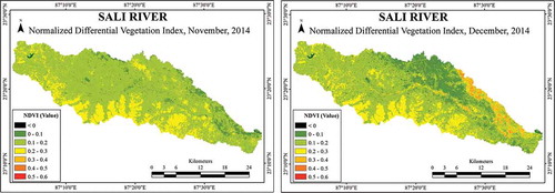
C.V. is an important indicator for the understanding of the nature of variation. In this study, we have computed pixel-wise C.V. and we have found that very high degree of variation (C.V. >80%) found over water logging area, such as over Gangdua Dam and near the confluence point of Sali River (Figure 7 (right)). High degree of variation (C.V. = 60% to 80%) is associated with the agricultural field with the irrigation facility, located in the north-eastern part of the watershed, e.g., Paschim Dubrajpur, Kamalpur, Palashbani and so on. A moderate degree of variation (C.V. = 40–60%) dominantly found in the northern, north-eastern, and eastern part of the basin, mainly along the Damodar River and around irrigation-fed agricultural land. Besides this, several small and discrete patches of moderate variation of NDVI (40–60%) were found in the area throughout the basin in a scattered manner. However, a lower degree of NDVI variation (C.V. = 20–40%) dominated throughout the Sali River basin and covered more than half of its area. It is mainly located in the southern and western parts of the river basin, which is associated with Sal forest, shrub and single crop agricultural land. Lowest variation with C.V. less than 20% was found in very few places covered with forest and shrub. Here, it can be said that the quality of vegetation varies within a year and the variation over vegetation-covered area is comparatively lower than the non-vegetation area (agricultural field and built-up area). Forest cover areas of this watershed represents a variation of NDVI throughout the year and it ranges from 20–60% C.V. as well as S.D. of this area showing similar kinds of result (Figure 7 (left)). So, we can say that there is a variation of NDVI within a year.

Figure 7. Pixel wise variation of NDVI, S.D. of NDVI (left) and C.V. of NDVI (right).

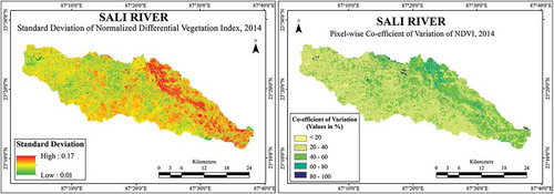
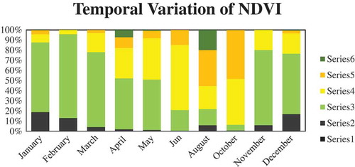
Figure 8. Month wise Variation of NDVI.

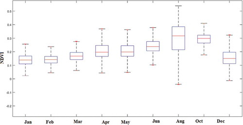
With the help of the percentage bar graph and box-plot graph, it becomes very clear that the NDVI value of this region is not static in nature (Figure 8 and 9). It varies from time to time. During the first three months (January, February and March), lower amount of NDVI (0.2–0.3) dominated over 70% of the area of the basin.

3.3 Nature of variation of vegetation status of Sali River watershed

So, from the above study, we have found that the NDVI of Sali River is not uniform in nature and it has spatial as well as temporal variation in the vegetation. VS for the months of January, February, March, April and May are more or less similar in nature. Although May monthindicates some sort of transition phase (Figures 4 (left), 7, and 9), the month of June can be said as absolutely transition month. Apart from these, August and October represent higher concentration inthe high NDVI region. Rest of them, i.e., November and December, are more or less equal to pre-monsoon seasons, like January, February, etc.

Figure 9. Comparative representation of NDVI.

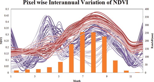
Figure 10 was constructed based on the selected sample location points and their respective NDVI representations. If we judge the graph carefully, it can be found that there are two distinct patterns of NDVI reflection which can be easily identifiable such as single and multiple peaks of NDVI. The single peak during monsoon season is the representative of forest or natural vegetation (Figure 11). On the other hand, multiple (three peaks) peaks represent the agricultural field, settled area and so on. So, the natural variation of vegetation actually follows the strong pattern of precipitation.

Figure 10. Month wise distribution of NDVI.

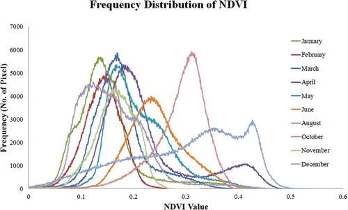
Figure 11. Intra-annual variation of NDVI and distribution of rainfall in this area.

4. Discussion

Understanding vegetation dynamics is an important aspect of the environmental monitoring. In this study, we have tried to detect the natural variability of NDVI using Landsat 8 data to get more accurate information about the vegetation. The temporal resolution of Landsat 8 dataset is about 16 days and it is generally obstructed by the presence of cloud during monsoon season. Along with this, vegetation status is not uniform throughout the year. As Sal forest is deciduous in nature, from May to June, it remains low to medium; from August to October, it achieves high NDVI; and from November to December, again it represents low-to-medium NDVI. During the month of January to April, the forest area represents low NDVI because during this time very few leaves were available in the forest area to reflect NDVI signature. On the other hand, rest of the forest areas, which is associated with diversified land use and land cover such as bare land, agricultural land, settled area, waterbody and so on, represent diversified nature of NDVI throughout the year. From our sample locations, we have found the same kinds of result. As these areas are associated with agricultural fields and irrigation facilities, resulting most of the land types are two crops and in certain cases, it is three crops. Due to this reason, during months of April, August and December, these areas were associated with relatively high NDVI. This has led us to represent the consensus that natural forest has accustomed to regional climate and based on the climatic character, vegetation changes their dynamics through the formation of a single peak within a year. However, the rest of them is associated with human modification through agricultural practices leading to two or three oscillating peaks within a year. So, there is a distinct nature of NDVI variation which is dependent on the nature of land use and land cover characters (Figure 11.).

Studies from different parts of the monsoon-dominated countries indicated that variation of NDVI is related to El Nino-Southern Oscillation (ENSO) and its associated “teleconnection” for Africa, Australia and South America (Anyamba & Eastman, 1996; Eastman & Fulk, 1993; Li & Kafatos, 2000; Sarkar & Kafatos, 2004), whereas others have found its association with sea surface temperature anomaly (Myneni et al., 1996; Sarkar & Kafatos, 2004). Cissé et al. (2016) studied on the monsoon-dominated region of Ferlo Basin (Senegal) and found that precipitation amount and its duration control the spatiotemporal variation in vegetation growth. In the case of Indian subcontinent, Sarkar and Kafatos (2004) found that meteorological parameters play a dominant role in NDVI variation. In this case, it has been found from Figure 11 that there were two kinds of distribution in the variation of NDVI, such as variation of a single peak (in brown colour) and variation of multiple peaks (in violet colour). Along with this, it was also found that the build-up areas and agricultural fields were associated with multiple peaks of NDVI distribution and on the other hand, forest-dominated areas were associated with a single peak of NDVI distribution which is following the rainfall graph. Therefore, it can be said that rainfall pattern is playing a dominant role on the variation of NDVI which is quite similar to the findings of Sarkar and Kafatos (2004) and Cissé et al. (2016). In this regard, it can be said that the status of vegetation varies with the variation in precipitation and on the other hand, rainfall duration and its intensity are affected by climate change (National Research Council, 1999; Trenberth, Zhang, & Gehne, 2017). Therefore, it can be presumed that long and continuous and increasing intensity of climate change may have led to a definite impact on natural vegetation.

Another concern is that the recent studies show that the climate change is an evident fact (National Research Council, 1999). It is also a serious concern for human as well as for other living beings on this planet Earth. Due to climate change, it was found that the temporal duration of precipitation decreased as well as the intensity of rainfall has increased (Trenberth et al., 2017). We have found that forest in this region, as well as other areas, is strongly associated with the annual nature of precipitation. So, long, continuous and increasing intensive climate change may have a definite impact on natural vegetation, particularly the availability of water.

5. Conclusion

In this study, intra-annual variability of vegetation dynamics has been studied using remotely sensed Landsat 8 data and it has been found that vegetation status is not uniform especially over time. The highest concentration of NDVI or good quality of vegetation has been found over the forest cover area as well as over the agricultural area with irrigation facility. Variation of vegetation status over irrigation-fed region is very high and it became less in case of forest area due to having minor changes in vegetation quality and lowest over the rest of the area. Vegetation status of this region is changing with respect to the changing nature of monsoon precipitation. Therefore, it can be said that intra-annual variation of vegetation status should be considered during the assessment of vegetation status of any region. In this study, we have focused only one year and further study can be done considering long temporal scale to understand the changing nature of vegetation dynamics with respect to time as well to detect the impact of climate change on vegetation dynamics.

Compliance with ethical standards

On behalf of all authors, the corresponding author states that there is no conflict of interest.

Acknowledgements

We cordially thank the Dept. of Geography, The University of Burdwan, for the infrastructural assistance such as use of different kinds of remote sensing and GIS software and writing software. We would also like to express our thanks to the editors and reviewers for their valuable comments and suggestion in regard to the upgradation of this manuscript.

Disclosure statement

No potential conflict of interest was reported by the authors.

References

- Alberdi, I., Nunes, L., Kovac, M., Bonheme, I., Cañellas, I., Rego, F. C., & Gasparini, P. (2019). The conservation status assessment of Natura 2000 forest habitats in Europe: Capabilities, potentials and challenges of national forest inventories data. Annals of Forest Science, 76(2), 34.
- Anyamba, A., & Eastman, J. R. (1996). Interannual variability of NDVI over Africa and its relation to El Niño/Southern Oscillation. Remote Sensing, 17(13), 2533–2548.
- Bannari, A., Morin, D., Bonn, F., & Huete, A. R. (1995). A review of vegetation indices. Remote Sensing Reviews, 13(1–2), 95–120.
- Betts, A. K., Ball, J. H., Beljaars, A. C., Miller, M. J., & Viterbo, P. A. (1996). The land surface‐atmosphere interaction: A review based on observational and global modeling perspectives. Journal of Geophysical Research: Atmospheres, 101(D3), 7209–7225.
- Bjorkman, A. D., Criado, M. G., Myers-Smith, I. H., Ravolainen, V., Jónsdóttir, I. S., Westergaard, K. B., … Heiðmarsson, S. (2019). Status and trends in Arctic vegetation: Evidence from experimental warming and long-term monitoring (pp. 1–15). Ambio, Advance online publication. doi:10.1007/s13280-019-01161-6
- Carlson, T. N., & Ripley, D. A. (1997). On the relation between NDVI, fractional vegetation cover and leaf area index. Remote Sensing of Environment, 62(3), 241–252.
- Chase, T. N., Pielke, R. A., Kittel, T. G., Nemani, R., & Running, S. W. (1996). Sensitivity of a general circulation model to global changes in leaf area index. Journal of Geophysical Research: Atmospheres, 101(D3), 7393–7408.
- Cihlar, J., Laurent, L. S., & Dyer, J. A. (1991). Relation between the normalized difference vegetation index and ecological variables. Remote Sensing of Environment, 35(2–3), 279–298.
- Cissé, S., Eymard, L., Ottlé, C., Ndione, J. A., Gaye, A. T., & Pinsard, F. (2016). Rainfall intra-seasonal variability and vegetation growth in the Ferlo Basin (Senegal). Remote Sensing, 8(1), 66.
- Cuomo, V., Lanfredi, M., Lasaponara, R., Macchiato, M. F., & Simoniello, T. (2001). Detection of interannual variation of vegetation in middle and southern Italy during 1985–1999 with 1 km NOAA AVHRR NDVI data. Journal of Geophysical Research: Atmospheres, 106(D16), 17863–17876.
- de Jong, R., de Bruin, S., de Wit, A., Schaepman, M. E., & Dent, D. L. (2011). Analysis of monotonic greening and browning trends from global NDVI time-series. Remote Sensing of Environment, 115(2), 692–702.
- Demisse, G. B, Tadesse, T, Bayissa, Y, Atnafu, S, Argaw, M, & Nedaw, D. (2018). Vegetation condition prediction for drought monitoring in pastoralist areas: a case study in ethiopia. International Journal Of Remote Sensing, 39(14), 4599–4615. doi:10.1080/01431161.2017.1421797
- Detsch, F., Otte, I., Appelhans, T., Hemp, A., & Nauss, T. (2016). Seasonal and long-term vegetation dynamics from 1-km GIMMS-based NDVI time series at Mt. Kilimanjaro, Tanzania. Remote Sensing of Environment, 178, 70–83.
- Dubovyk, O., Landmann, T., Erasmus, B. F., Tewes, A., & Schellberg, J. (2015). Monitoring vegetation dynamics with medium resolution MODIS-EVI time series at sub-regional scale in southern Africa. International Journal of Applied Earth Observation and Geoinformation, 38, 175–183.
- Eastman, J. L., Coughenour, M. B., & Pielke, R. A., Sr. (2001). Does grazing affect regional climate?. Journal of Hydrometeorology, 2(3), 243–253.
- Eastman, J. R., & Fulk, M. (1993). Long sequence time series evaluation using standardized principal components. Photogrammetric Engineering and Remote Sensing, 59, 6.
- Egbert, S. L., Park, S., Price, K. P., Lee, R. Y., Wu, J., & Nellis, M. D. (2002). Using conservation reserve program maps derived from satellite imagery to characterize landscape structure. Computers and S in Agriculture, 37(1–3), 141–156.
- Eswaran, H., Lal, R., & Reich, P. F. (2001). Land degradation: An overview. Responses to Land Degradation, In E. Bridges, I. Hannam, L. Oldeman, F. Penning de Vries, S. Scherr, & S. Sompatpanit. (Eds.), Proceesings of 2nd International Conference on Land Degradation and Desertification. Khon Kaen, Thailand, (pp. 20-35). New Delhi: Oxford Press. 20–35.
- Fensholt, R. (2004). Earth observation of vegetation status in the Sahelian and Sudanian West Africa: Comparison of Terra MODIS and NOAA AVHRR satellite data. International Journal of Remote Sensing, 25(9), 1641–1659.
- Fensholt, R., & Proud, S. R. (2012). Evaluation of earth observation based global long term vegetation trends—Comparing GIMMS and MODIS global NDVI time series. Remote Sensing of Environment, 119, 131–147.
- Foley, J. A., Kutzbach, J. E., Coe, M. T., & Levis, S. (1994). Feedbacks between climate and boreal forests during the Holocene epoch. Nature, 371(6492), 52–54. https://doi.org/10.1038/371052a0
- Fu, Y., Chen, H., Niu, H., Zhang, S., & Yang, Y. (2018). Spatial and temporal variation of vegetation phenology and its response to climate changes in qaidam basin from 2000 to 2015. Journal of Geographical Sciences, 28(4), 400–414. doi:10.1007/s11442-018-1480-2
- Gray, T. I., Jr, & Tapley, B. D. (1985). Vegetation health: Nature’s climate monitor. Advances in Space Research, 5(6), 371–377.
- Guerschman, J. P., Hill, M. J., Renzullo, L. J., Barrett, D. J., Marks, A. S., & Botha, E. J. (2009). Estimating fractional cover of photosynthetic vegetation, non-photosynthetic vegetation and bare soil in the Australian tropical savanna region upscaling the EO-1 Hyperion and MODIS sensors. Remote Sensing of Environment, 113(5), 928–945.
- Guo, X., Zhang, H., Yuan, T., Zhao, J., & Xue, Z. (2015). Detecting the temporal scaling behavior of the normalized difference vegetation index time series in China using a detrended fluctuation analysis. Remote Sensing, 7(10), 12942–12960.
- He, C., Zhang, Q., Li, Y., Li, X., & Shi, P. (2005). Zoning grassland protection area using remote sensing and cellular automata modeling—A case study in Xilingol steppe grassland in northern China. Journal of Arid Environments, 63(4), 814–826.
- Hou, G., Zhang, H., & Wang, Y. (2011). Vegetation dynamics and its relationship with climatic factors in the Changbai Mountain Natural Reserve. Journal of Mountain Science, 8(6), 865–875.
- Huemmrich, K. F., Black, T. A., Jarvis, P. G., McCaughey, J. H., & Hall, F. G. (1999). High temporal resolution NDVI phenology from micrometeorological radiation sensors. Journal of Geophysical Research: Atmospheres, 104(D22), 27935–27944.
- Jeong, S. J., HO, C. H., GIM, H. J., & Brown, M. E. (2011). Phenology shifts at start vs. end of growing season in temperate vegetation over the Northern Hemisphere for the period 1982–2008. Global Change Biology, 17(7), 2385–2399.
- Jia, K., Liang, S., Gu, X., Baret, F., Wei, X., Wang, X., … Li, Y. (2016). Fractional vegetation cover estimation algorithm for Chinese GF-1 wide field view data. Remote Sensing of Environment, 177, pp.184–191.
- Knight, J. F., Lunetta, R. S., Ediriwickrema, J., & Khorram, S. (2006). Regional scale land cover characterization using MODIS-NDVI 250 m multi-temporal imagery: A phenology-based approach. GIScience & Remote Sensing, 43(1), 1–23.
- Lanfredi, M., Lasaponara, R., Simoniello, T., Cuomo, V., & Macchiato, M. (2003). Multiresolution spatial characterization of land degradation phenomena in southern Italy from 1985 to 1999 using NOAA‐AVHRR NDVI data. Geophysical Research Letters, 30, 2.
- Langley, S. K., Cheshire, H. M., & Humes, K. S. (2001). A comparison of single date and multitemporal satellite image classifications in a semi-arid grassland. Journal of Arid Environments, 49(2), 401–411.
- Lanorte, A., Lasaponara, R., Lovallo, M., & Telesca, L. (2014). Fisher–Shannon information plane analysis of SPOT/VEGETATION Normalized Difference Vegetation Index (NDVI) time series to characterize vegetation recovery after fire disturbance. International Journal of Applied Earth Observation and Geoinformation, 26, 441–446.
- Li, Z., & Kafatos, M. (2000). Interannual variability of vegetation in the United States and its relation to El Nino/Southern Oscillation. Remote Sensing of Environment, 71(3), 239–247.
- Lu, L., Kuenzer, C., Wang, C., Guo, H., & Li, Q. (2015). Evaluation of three MODIS-derived vegetation index time series for dryland vegetation dynamics monitoring. Remote Sensing, 7(6), 7597–7614.
- Martínez, B., & Gilabert, M. A. (2009). Vegetation dynamics from NDVI time series analysis using the wavelet transform. Remote Sensing of Environment, 113(9), 1823–1842.
- Myneni, R. B., Los, S. O., & Tucker, C. J. (1996). Satellite‐based identification of linked vegetation index and sea surface temperature Anomaly areas from 1982–1990 for Africa, Australia and South America. Geophysical Research Letters, 23(7), 729–732.
- Naidoo, R., Gerkey, D., Hole, D., Pfaff, A., Ellis, A. M., Golden, C. D., … Fisher, B. (2019). Evaluating the impacts of protected areas on human well-being across the developing world. Science Advances, 5(4), eaav3006.
- Nanzad, L., Zhang, J., Tuvdendorj, B., Nabil, M., Zhang, S., & Bai, Y. (2019). Ndvi anomaly for drought monitoring and its correlation with climate factors over mongolia from 2000 to 2016. Journal of Arid Environments, 164, 69–77. doi:10.1016/j.jaridenv.2019.01.019
- National Research Council. (1999). Global environmental change: Research pathways for the next decade. Washington DC: National Academies Press. doi:10.17226/5992
- Nemani, R. R., Keeling, C. D., Hashimoto, H., Jolly, W. M., Piper, S. C., Tucker, C. J., … Running, S. W. (2003). Climate-driven increases in global terrestrial net primary production from 1982 to 1999. science, 300(5625), 1560–1563.
- Nordberg, M. L., & Evertson, J. (2005). Vegetation index differencing and linear regression for change detection in a Swedish mountain range using Landsat TM® and ETM+® imagery. Land Degradation & Development, 16(2), 139–149.
- Pal, S. C., Chakrabortty, R., Malik, S., & Das, B. (2018). Application of forest canopy density model for forest cover mapping using LISS-IV satellite data: A case study of Sali watershed, West Bengal. Modeling Earth Systems and Environment, 4(2), 853–865.
- Pettorelli, N., Vik, J. O., Mysterud, A., Gaillard, J. M., Tucker, C. J., & Stenseth, N. C. (2005). Using the satellite-derived NDVI to assess ecological responses to environmental change. Trends in Ecology & Evolution, 20(9), 503–510.
- Rouse, J. W., Haas, R. H., Deering, D. W., & Schell, J. A. (1974). Monitoring The Vernal Advancement and Retrogradation (Green Wave Effect) Of Natural Vegetation. Retrieved from https://ntrs.nasa.gov/archive/nasa/casi.ntrs.nasa.gov/19740004927.pdf
- Sarkar, S., & Kafatos, M. (2004). Interannual variability of vegetation over the Indian sub-continent and its relation to the different meteorological parameters. Remote Sensing of Environment, 90(2), 268–280.
- Scanlon, T. M., Albertson, J. D., Caylor, K. K., & Williams, C. A. (2002). Determining land surface fractional cover from NDVI and rainfall time series for a savanna ecosystem. Remote Sensing of Environment, 82(2–3), 376–388.
- Schucknecht, A., Erasmi, S., Niemeyer, I., & Matschullat, J. (2013). Assessing vegetation variability and trends in north-eastern Brazil using AVHRR and MODIS NDVI time series. European Journal of Remote Sensing, 46(1), 40–59.
- Sobrino, J. A., & Julien, Y. (2011). Global trends in NDVI-derived parameters obtained from GIMMS data. International Journal of Remote Sensing, 32(15), 4267–4279.
- Teferi, E., Uhlenbrook, S., & Bewket, W. (2015). Inter-annual and seasonal trends of vegetation condition in the Upper Blue Nile (Abay) Basin: Dual-scale time series analysis. Earth System Dynamics, 6(2), 617–636.
- Telesca, L., & Lasaponara, R. (2006). Quantifying intra-annual persistent behaviour in SPOT-VEGETATION NDVI data for Mediterranean ecosystems of southern Italy. Remote Sensing of Environment, 101(1), 95–103.
- Telesca, L., Lasaponara, R., & Lanorte, A. (2008). Intra-annual dynamical persistent mechanisms in mediterranean ecosystems revealed SPOT-VEGETATION time series. Ecological Complexity, 5(2), 151–156.
- Trenberth, K. E., Zhang, Y., & Gehne, M. (2017). Intermittency in precipitation: Duration, frequency, intensity and amounts using hourly data. Journal of Hydrometeorology, 18(5), 1393–1412.
- Tucker, C. J., & Sellers, P. J. (1986). Satellite remote sensing of primary production. International Journal of Remote Sensing, 7(11), 1395–1416.
- UN report on environment https://wedocs.unep.org/bitstream/handle/20.500.11822/27539/GEO6_2019.pdf?sequence=1&isAllowed=y (Accesses on 08 June, 2019)
- Xiao, J., & Moody, A. (2005). A comparison of methods for estimating fractional green vegetation cover within a desert-to-upland transition zone in central New Mexico, USA. Remote Sensing of Environment, 98(2–3), 237–250.
- Xiao, X. (2004). Modeling gross primary production of temperate deciduous broadleaf forest using satellite images and climate data. Remote Sensing of Environment, 91(2), 256–270.
- Xie, Y., Sha, Z., & Yu, M. (2008). Remote sensing imagery in vegetation mapping: A review. Journal of Plant Ecology, 1(1), 9–23.
- Yang, W., You, Q., Fang, N., Xu, L., Zhou, Y., Wu, N., Ni, C., Liu, Y., Liu, G., Yang, T., & Wang, Y. (2018). Assessment of wetland health status of poyang lake using vegetation-based indices of biotic integrity. Ecological Indicators, 90, 79–89. doi:10.1016/j.ecolind.2017.12.056
- Zhao, J., Wang, Y., Hashimoto, H., Melton, F. S., Hiatt, S. H., Zhang, H., & Nemani, R. R. (2013). The variation of land surface phenology from 1982 to 2006 along the Appalachian trail. IEEE Transactions on Geoscience and Remote Sensing, 51(4), 2087–2095.