Investigation of Maize Lethal Necrosis (MLN) severity and cropping systems mapping in agro-ecological maize systems in Bomet, Kenya utilizing RapidEye and Landsat-8 Imagery

ABSTRACT

Spatiotemporal information on crops and cropping systems can provide useful insights into disease outbreak mechanisms in croplands. In September 2011, a severe outbreak of Maize Lethal Necrosis (MLN) disease was reported in Bomet County, Kenya. We aimed to detect severely MLN-infected fields and discriminate mono, inter, and continuous maize cropping systems. We collected in-situ MLN severity observations and acquired multi-date and multi-sensor data viz., RapidEye (RE), Sentinel-1 (S1), digital elevation model (DEM), and Landsat-8 (L8) imagery. A hierarchical classification approach was used to map the cropping systems and severely MLN-infected fields during the short rainy season (September 2014–February 2015) using the random forest (RF), one-class support vector machine (OCSVM) and biased SVM (BSVM) classifiers. RF showed better performance when a balanced multi-class dataset was available. Both OCSVM and BSVM did not lead to an accurate high severity MLN class separation. Moreover, the BSVM classifier was able to separate the mono and intercropping systems. During the long rainy season (March–August 2015), only maize crop data were available, hence the BSVM as one class classifiers (OCC) was used and maize fields were successfully mapped even with high confusion rate. Furthermore, the distribution of maize intercropping system increased in low rainfall sites, and the continuous cropping system limited to only 31% of total maize cropland.

KEYWORDS:

• Maize Lethal Necrosis disease
• cropping systems
• Machine learning

1. Introduction

Maize farming is the backbone of food and nutrition security in Kenya. The area under maize in the country increased from 1,700,000 ha in 2008 to 2,159,322 ha in 2012, which is the highest maize area increment since 1961. Maize production in Kenya also increased from 1,382,643 tons in 2012 to 3,513,171 tons in 2014, although the country still imports tonnes of maize from neighbouring countries like Tanzania each year to meet the consumption gap (Indexmundi, 2019). In general, maize production in eastern and central Africa is threatened by many biotic and abiotic constraints. One of the challenging maize production problems in this region is the Maize Lethal Necrosis (MLN) disease. The disease is caused by the co-infection of Maize Chlorotic Mottle Virus (MCMV) and the cereal viruses in the Potyviridae group such as Sugarcane Mosaic Virus (SCMV), Maize Dwarf Mosaic Virus, or Wheat Streak Mosaic Virus. SCMV is prevalent in Africa for nearly 50 years, but MCMV is much more recent and more destructive compared to SCMV (Braidwood et al., 2017). Also, Johnsongrass Mosaic Virus which has recently known to be present in the eastern Africa contributes to the emergence of the MLN disease in the region (Stewart et al., 2017). In combination, these viruses rapidly produce a synergistic reaction called MLN. It seriously damages or kills the infected maize plants at any growing stage (Kiruwa et al., 2016). MLN disease is not particularly new and has been identified for first time in the United States of America in 1976 (Nault et al., 1978).

The foremost problem is the fact that MLN outbreaks threaten food and nutrition security in eastern and central Africa. In Kenya, first reports of an unknown disease outbreak were observed in September 2011 in Bomet County. Further virological analyses identified the unknown disease as MLN. This problem has attracted further attention, when in 2012 the maize-crop-losses due to the MLN outbreak reached up to 90% (Mahuku et al., 2015). In 2014, Kipsawet near Bomet County was identified as a MLN hotspot area in Kenya. To overcome MLN outbreaks, different agronomical, biological, entomological, and pathological management approaches have been tested (Marenya et al., 2018). Planting MLN-free maize seeds, introducing MLN-resistant maize varieties, and practicing maize crop rotations have been proposed to surmount the problems caused by MLN, although the disease cannot be completely eradicated. Osunga et al. (2017) studied the relevance of some ecological variables on the spatial distribution of MLN disease in Bomet County using spatial regression modelling routine. With exception of temperature, they found that soil moisture, rainfall, and slope were the most influential variables on MLN occurrences. MLN disease is not only influenced by ecological variables, but other factors such as maize cropping system (i.e. mono, intercropping, continuous, and rotation cropping) which are reported to play a major role in the disease incidences, severity, and outbreak (Namikoye et al., 2017). However, only a few studies have focussed on the actual spatiotemporal distribution of MLN utilizing remotely sensed data.

In Bomet, the dominant maize cropping systems consist of mono (maize only), intercropping (maize and legumes such as cowpea or beans) and continuous or rotation cropping systems. In this region, farmers grow different maize varieties at varying planting dates during the growing season. Small-scale and highly fragmented farms is also a common practice in Bomet. These constraints make the MLN disease control difficult in this region. Moreover, discrimination of rain-fed crops from natural vegetation is challenging when both farms and surrounding vegetation are at the same phenological stage. Kiruwa et al. (2016) reported that the diagnosis of low and medium MLN severity based on visual symptoms is ineffective. One limitation in visually discriminating between low and medium MLN severity is that symptoms like stunting and chlorosis can also resemble nutrient deficiencies or maize mosaic disease. Because of this potential limitation, in this paper, the focus of detecting MLN-infected maize was only for high severity infestation levels which could lead to necrosis.

A possible solution to map the complex maize cropping systems accurately in Africa and specifically in Kenya is to use a multi-sensor and multi-temporal mapping approach coupled with robust and effective machine learning classification algorithms (Forkuor et al., 2015; Ianninia et al., 2013; Zillmann & Weichelt, 2014). Previous studies have emphasized that spectral vegetation indices (VIs) can enhance the multi-source crop classification results. Studies have also shown that the normalized difference vegetation index (NDVI), for instance, is sensitive to green vegetation and is not highly affected by other variables such as heterogeneous landscapes, atmospheric and sensor noises, soil background, or other ground elements in the image pixels (Bannari et al., 1995). It is also well acknowledged that, compared to other supervised image classification methods, random forest (RF) is a powerful and robust classification option to map agricultural fields. The method is a non-parametric machine learning algorithm which has the capability of using continuous and categorical datasets, easy to parameterize, and can deal with outliers in training data and is not sensitive to over-fitting (Horning, 2010). Also, RF performs better when dealing with multi-layers and multi-temporal data-sets (Cutler et al., 2007).

On the other hand, in the lack of sufficient samples, the one class classifier is a smarter choice (Braun & Hochschild, 2015; Heinl et al., 2009; Mack et al. 2014; Whiteside et al., 2011). The present paper addresses the need for providing remotely sensed spatiotemporal information of MLN disease occurrence to develop an effective controlling approach, what so far received less attention in the scientific literature. We looked at the possibility of mapping and linking maize cropping systems to high severity MLN occurrences. Specifically, this study investigated the use of RapidEye (RE) and Landsat 8 (L8) imagery to classify and map maize mono and intercropping systems and areas under high MLN infestation. For this purpose, machine learning RF (Breiman, 1996) and a one class classifier were utilized (Mack & Waske, 2017). We analysed the map of continuous/rotation cropping (in two continuous cropping season) and investigated whether the crop rotation was applied by farmers during MLN outbreaks in the region. Furthermore, for this study, it was of interest to establish the relationship between high severity MLN occurrence the corresponding cropping system and rainfall distribution in the study area.

2. Study area

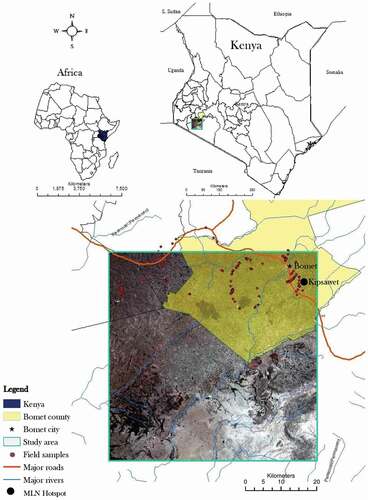
Bomet County is amongst the seven most high potential maize production zones in Kenya, and agriculture is the main economic activity in the County (Olwande et al., 2009). Bomet county has a population of 875,689 (2019 census), and an area of 1,997.9 km2. The most prevalent crops in Bomet are maize, beans, and cowpeas, while maize plays a major role in terms of food and nutrition security and income generation (Nyoro et al., 2004). The County is located in the semi-humid agro-ecological zone of Kenya and the mean annual maximum temperature is 28°C (Bryan et al., 2013). Average cumulative rainfall ranges from 500 to 2000 mm. Rainfall peaks twice a year in Bomet: in March–May (long rainy season) and in September–November (short rainy season). The vast majority of farmers in Bomet consider long rainy season to be their main maize cropping season and continuous cropping-system is known as the dominant cropping system in Bomet for a long time. However, during the short rainy season, fewer farmers grow maize (Hassan, 1996). The area under monocropping and intercropping system varies between the short and long rainy seasons (Ochieng et al., 2011). In regions with uncertainties in rainfall patterns, the majority of the farmers intercrop maize with beans. In addition, irrigated farming is also practiced in locations neighbouring the major rivers (Kimani et al., 2004). Specifically, the study area (01°18′16S, 034°52′04E, 00°44′43S, 035°25′23E) (Figure 1) covers 61 × 61 km² and the highest elevation is 1,962 m above sea level.

Figure 1. Bomet study area in Kenya and Maize Lethal Necrosis (MLN) hotspots collected in 2015.

3. Methodology

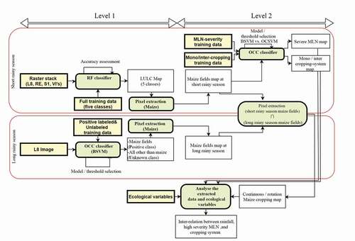
Prior to other steps, all satellite data were transformed to the recommended map projection (i.e. Universal Transverse Mercator: UTM WGS-84 ellipsoid) zone 36 south (Forkuor et al., 2014). To map maize fields, cropping system, and high severity MLN, a hierarchical classification approach was applied on the multi-sensor, multi-temporal satellite data using RF, one class support vector machine (OCSVM), and biased SVM (BSVM) classifiers. Available datasets were divided into two main cropping seasons, short rainy season (first season) from September to February and long rainy season (second season) from March to August. The peak of the rains is from September to November. As the first step, a raster-stack of RE, L8, Sentinel-1 (S1) and calculated VIs were generated for the short rainy season. During the same season, representative training data were collected using stratified random sampling approach (see section I below for details). Using the VIs, the field data and RF classifier, a general five-class land use and land cover(LULC) map (maize, non-maize, trees, water, and non-vegetation) was produced. Maize pixels were extracted from the classified map and reclassified for high severity MLN, mono- and intercropped maize systems using BSVM.

During the long rainy season, only maize fields’ data were available, consequently the BSVM classifier as a One Class Classifiers (OCC) was employed to classify maize fields on L8 imagery. Classified maize pixels during both the short and the long rainy seasons were overlaid, and common fields were mapped as continuous maize cropping system. Further, the inter-relations between-maize-cropping-system and high severity MLN with rainfall distribution were investigated. Figure 2 summarizes our data processing and analysis steps and procedures.

Figure 2. Workflow of the hierarchical classification approach using random forest and one class classifier during the short and long rainy seasons in Bomet, Kenya. The arrows illustrate data flow directions and dependencies, squares represent datasets while rounded rectangles were processes.

(i) In-situ data

We conducted four field campaigns between January to August 2015 during the short and long rainy seasons, respectively, following a stratified random sampling method. During the first rainy season, three field campaigns (between January to April 2015) were conducted to collect data on different LULC classes (water bodies, grasslands, soil, houses, and tarmac roads), crop type and conditions (physical condition, growth stage, and MLN severity), cropping system (mono/intercropping) and crop rotation (continuous/rotational). During the long rainy season, one field campaign only was conducted on August 2015 to collect reference data on the location of maize fields. All in-situ data were georeferenced using a global positioning system (GPS) of ±3 m error. Polygons spanning 30 × 30 m and at least 5 m away from the edge of each field were sampled to avoid the edge effect. For further inspections of the cropping systems and crop age in the sample polygons, geo-tagged photographs of each cropping system were recorded. Also, in order to minimize the soil background effect on the imagery spectral reflectance, maize fields younger than 3 weeks were excluded from data collection.

(ii) Satellite data

The satellite data consist of 5-meter bi-temporal RE imagery acquired between 9 December 2014 and 23 January 2015 which covered the short rainy season. In addition, 12 cloud-free 30-meter multi-temporal L8 images were acquired between November 2013 and August 2015. The L8 imagery covered both the short and the long rainy seasons. All L8 imagery were downloaded from the Landsat Surface Reflectance Climate Data Records (CDRs) database as Level 1 surface reflectance. Two 30-meter Shuttle Radar Topography Mission (SRTM) digital elevation model tiles and two S1 datasets in Interferometric wide swath mode, with dual VV (vertical transmit and vertical receive)/VH (vertical transmit and horizontal receive) polarizations were acquired for the same time period. The S1 data were utilized to improve classification accuracy (Forkuor et al., 2014).

(a) Pre-processing

(iii) SAR data

The SRTM DEM (digital elevation model) arc 1-sec imagery were cropped and resampled (bilinear interpolation) to L8 and RE imagery. These products were stacked with L8, RE, S1, and VIs to provide an input for RF classifier. In addition, the DEM was needed to perform atmospheric and topographic corrections on RE imagery to reduce the speckles and to geometrically correct the S1 imagery. A Lee filter of 7 × 7 pixels and Range–Doppler Terrain Correction methods were applied according to the procedures described in Ozdarici and Akyurek (2010). The filter was implemented by the SNAP software (from ESA) sentinel-1 toolbox using the post-filtering module. . Further, the backscatter of the corrected S1 imagery was converted to decibel (dB) units.

(iv) RapidEye

The RE tiles were atmospherically and geometrically corrected using atmospheric-topographic correction (ATCOR 3) software which requires SRTM DEM data (Richter & Schläpfer, 2005). Finally, the radiometric-geometric-corrected-tiles were mosaicked to produce a two RE imagery layers’ stack for the two different acquisition dates.

(v) Landsat 8

L8 imagery were cropped to RE image products, resampled and co-registered. Both RE and L8 imagery had cloud and clouds’ shadow cover which were manually masked (Kross et al., 2015).

(vi) Vegetation indices

Previous studies have emphasized the importance of VIs for crop classification (Bannari et al., 1995; Zillmann & Weichelt, 2014). VIs are more sensitive to “green” that is chlorophyll active vegetation than the single spectral bands. In the present study, several VIs such as NDVI, simple ratio (SR), red-edge NDVI (NDVIre), red-edge SR(SRre), green NDVI (gNDVI), and modified triangular vegetation index (MTVI2) were calculated using the visible, near-infrared, and red-edge bands of L8 or RE imagery. The original bands were used in combination with the calculated VIs as an input variables on the RF and other classifiers (Forkuor et al., 2014). The time-series NDVI dataset utilized in our study was extracted from 12 cloud-free L8 images which covered the period from November 2013 to August 2015.

(b) Classifiers

(i) Random Forest

It has been shown that RF classifier was able to handle large-scale high dimensional data with high/medium spatial resolution (Forkuor et al., 2014; Whiteside et al., 2011). Previous studies have also found that RF could perform better on multi-temporal dataset and is capable of dealing with noisy and highly correlated remotely sensed predictor variables (Braun & Hochschild, 2015). In this experiment, RF was employed to classify a raster-stack of RE, L8, VIs, and S1 which covers the short rainy season in the study area. The RF classifier takes random bootstrapped subsets from a training dataset and constructs several classification trees using each of these subsets. Branches in the trees are often thresholds defined for the measured (known) variables in the dataset. Whereas, leaves are the class labels assigned at the termini of the trees. RF classifier requires optimization of two user-defined parameters, which are number of trees (n-tree) and number of variables used to split the trees (m-try). The default value of m-try is the square root of the total number of the predictor variables. One-third of the training dataset which is not included in the bootstrapped training sample are left out as out-of-bag (OOB) subset. An OOB error for each tree is computed by predicting the class associated with its in-bag value. This process results in a classification confusion matrix which can be used to evaluate the classification results. Therefore, we calculated overall accuracy (OA), producer’s accuracy (PA) and user’s accuracy (UA) from the confusion matrix to evaluate the RF classifier performance. We set n-tree to 100, 500, and 1000 to help select the most optimal classification result. RF variable importance was, furthermore used to determine the optimal spectral variables (Kuhn, 2007). We tested RF classification experiments with six imbalanced classes and five balanced classes to produce a general LULC map. The experiment that provided a good fit to the data with the best classification performance was chosen.

(ii) One Class Classifier

Previous studies have emphasized that OCC algorithms have the advantage of coping with incomplete training data to map only one specific class of interest. In contrast to RF, OCC just classifies the target class. In the present study, at the long rainy season, the available sample data were constrained to maize fields. In addition, only one class such as monocropping or high severity MLN were targeted at the short rainy season, which makes the OCC classifier as an optimum classification option. On the other hand, a careful manual interpretation of the diagnostic plots such as the class separation and suitability of a specific threshold is necessary for parameter-setting and evaluation which makes the OCC classifier to be less suitable for operationalization (Mack et al. 2014). In this study, OCSVM as a P-classifier (P represents positive labelled pixels as class of interest) was employed to cope with incomplete datasets at long rainy season. Because of the lack of complete validation samples, the so-called performance metrics are unidentifiable in OCSVM approach. High severity MLN (target class) was employed to train the OCSVM classifier (P samples) for the short rainy season period. In contrast to a common supervised classifier, OCC classifiers reject the classification of a pixel if it does not sufficiently match one of the known classes. Consequently, the map production cost can be significantly reduced. This is particularly important, if a complete reference data are missing and the user is interested in only one or few classes. A serious disadvantage in the case of OCSVM, is the absence of a confusion matrix, because the labelled samples are only available for the “Positive class” of interest, but not for the other classes (Mack, 2017). OCSVM has been performed in both automatic and manual model-selection mode. P-classifiers such as OCSVM performances are based on 1) similarity measure like the distance between the positive training samples and the target pixel to be classified and 2) the threshold of the similarity measure to identify the target class membership. Insignificant class overlap or uniform distribution of negative and positive classes can lead to an optimum OCSVM classification results. In this experiment, PU-performance metrics (puF) diagnostic plots were extracted and data evaluation performed manually. The puF is based on the true positive rate (tpr) which estimates the probability of classifying positive samples (true positives) out of the positive training samples (the total actual positives). puF plots are based on two parameters: 1) “nu” which sets an upper bound on the fraction of outliers (training examples regarded out-of-class) and a lower bound on the number of training samples used as support vector. Setting “nu” to a large value results in a higher number of outliers. This can cause large false positives rate. 2) “Sigma” is the radial basis function (RBF) kernel that is used in various kernelized learning algorithms, specifically in SVM classification. Gaussian kernel function ($\mathrm{K}$) as a non-linear function of Euclidean distance is:

$\mathrm{K}\left(\mathrm{x},{\mathrm{x}}^{\prime }\right)=\mathrm{e}\mathrm{x}\mathrm{p}\left(-\frac{{\left|\left|\mathrm{x}-{\mathrm{x}}^{\prime }\right|\right|}^2}{2{\sigma }^2}\right)$

SVM classifier tries to find similarities between x (positive training sample) and x’ (pixels to be classified) where${\left|\left|\mathrm{x}-{\mathrm{x}}^{\prime }\right|\right|}^2$, is the Euclidean distance between $\mathrm{x}$ and${\mathrm{x}}^{\prime }$ and σ is a standard deviation which determines the width for Gaussian distribution. For a larger${\sigma }^2$ the Gaussian function will tend to fall off slowly and cause low variance and high bias. For a smaller sigma, the decision boundary tends to be high variance and less biased and cause over-fitting. “nu” and “Sigma” parameters should be set manually and changed from one classification to another. Also, manual model selection table provides tpr and Probability of Positive Prediction (ppp). The ppp estimates the probability of classifying a sample as positive out of the unlabelled samples which are derived at the threshold 0 (Ө₀). This paper utilized Bayes’ rule for OCC with positive and unlabelled (PU) data. The PU-performance metrics (puF) is related to the F-score and can be derived from PU data. PU area under the curve (puAuc) is related to the area under the receiver operating curve. The model selection table parameters such as puAuc (positive/unlabelled area under curve) and performance metrics were utilized to choose an optimal model. On the other hand, puAuc is a threshold independent parameter, which calculates the performance over the whole range of possible thresholds. Thus, it also considers unsuitable thresholds. It comprises the density histogram of the predicted image (dark grey), the distribution of positive (dark blue box), and unlabelled predictions (light grey box). These are the predictions of cross-validated, positive, and unlabelled training samples. The light-blue box shows the calibration predictions (the prediction on the positive training data with the model, which trained on the full training data).

BSVM uses training with the class of interest as a positive class, and other class as unlabelled class. With the test set (±test), an accuracy assessment for the binary classification results over the whole range of possible thresholds can be performed.

In this study, confusion matrices and accuracy measures for the given classes were provided for two types of thresholds: 1) Ө₀ which was obtained by the BSVM, and 2) the Ө_opt which is the highest K. There was a third map threshold (Ө_map) which can be obtained by Bayes’ rule, but it is not discussed in this study. Usually, Ө₀ leads to very high PA (less omission or high true positive rate) and very low UA (high commission or false-positive rate), while Ө_map improves it. PU-classifiers overcome P-classifier problems by bringing into account the unlabelled data. It gives the target classes a label “Positive” and the remaining classes the label “Negative/Unlabelled.” With too few unlabelled training samples it will be impossible to get close to the optimal decision boundary.

Also, in some extends, a user-oriented strategy used to support the handling of OCC according to the work of Mack et al. (2014). The detailed evaluation of the results as it has been described by Mack et al. (2014) is out of the objectives of this study.

4. Results and discussion

The imbalanced model of classifying the six classes (maize, grassland, tree, non-vegetation, water, and non-maize crops) using RF resulted in an OA of 65.1%, K of 0.58, and OOB error of 1.64% with 500 RF trees. When 100 trees were used, the model yielded an OA of 63% and K of 0.56. In theory, more RF trees should produce a better classification result, but the improvement in RF model performance decreases as the number of trees increases (Oshiro et al., 2012). It is worth noting that the gain in the classification accuracy is lower than the cost of computation time when learning more RF trees. To avoid negative effect of the imbalanced classes, we combined the non-maize and grassland classes in one class. On the other hand, the RF model with five balanced classes and 500 trees resulted in an OA of 89.63% and K of 0.74. The individual class accuracy was 83.57% for maize, 92.75% for non-maize, 98.59% for tree, 85.15% for non-vegetation, and 92.65% for water. Overall, the balanced model performed better than the imbalanced model for producing an accurate LULC map. In addition, analysing the RF variable importance by-product indicated that S1 layer had the highest mean decrease in accuracy as compared to other layers.

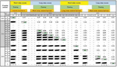
The results of the LULC classification were limited by cloud cover as such it was difficult to acquire a complete set of multi-temporal NDVI dataset. Figure 3 shows that correlation between NDVI temporal profiles is higher at the adjacent maize development phases in each season. For instance, between May and June which are maize tasselling and maturation development stages, respectively, the correlations between NDVI profiles were high (Figure 3). These correlations dropped towards September, which is the maize harvesting stage. Interestingly, the correlation between NDVI profiles between June 2015 and overlapped area at June 2014 is only 0.39 which is considered very low (Figure 3).

Figure 3. Correlation between maize normalized difference vegetation index (NDVI) profiles (2013–2015) during the short and long rainy seasons at Bomet, Kenya. Numbers indicate the correlation between NDVI profiles. (-): No data were available.

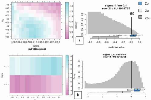
The performance metrics of the OCSVM as P-classifier model that were used to map the high severity MLN maize is presented in Table 1 and Figure 4. In the present study, the results of the P-classifier without manual model selection showed that the positive hold-out predictions (dark blue box) are located at the far right and separated from the negative hold-out predictions (light grey box) at the far-left side (Figure 4). Nevertheless, the confusion is high as some of the positive holdout predictions located at negative region. Additionally, there was no discriminative low-density region between these two classes. Our results demonstrated that a model based on the high puAuc did not show better performance comparing to the default model and leaded to high confusion rate. The grid (Figure 4(a)) shows that the puF dropped sharply at “Sigma” values smaller than 0.11 and greater than 1.4 and “nu” higher than 0.3. However, it is possible to find a finer grid (Figure 4(b)) around “Sigma” = 0.11 to achieve a better model. The diagnostic plot implies that the positive-labelled target class (high severity MLN) and the negative-labelled class (all other MLN severity levels) in both try (before and after manual interpretation and selection) can hardly be separated without high confusion rate.

Table 1. Manual model selection for one class support vector machine (OCSVM) classification of Maize Lethal Necrosis (MLN) severity, model parameters, and performance metrics

Row	sigma	nu	tpr	puP	ppp	puAuc	puF	puF1
11	0.11	0.05	0.93	0.41	0.344	0.93	2.6	0.57
12	0.11	0.10	0.88	0.42	0.316	0.92	2.5	0.57

Figure 4. Default one class support vector machine (OCSVM) positive (P) classifier results for mapping Maize Lethal Necrosis (MLN) severity. (a) is the corresponding puF diagnostic plot, and (b) is the MLN severity classification after puF manual model selection. Zp: distribution of positive prediction, Zu: distribution of unlabelled predictions, Zpu: density histogram of the predicted image.

With the test set (±test), an accuracy assessment for the binary classification results over the whole range of possible thresholds was performed (Table 2). Because of limited number of available training samples, it was not possible to provide bigger P training samples to cover wider spectral ranges. Low-density area in a histogram usually interprets as a good class separation. From the BSVM classification results, it was clear that high confusion rate existed between high severity MLN and healthy maize fields even after thresholding (Figure 5). It is important to highlight the fact that a clear low-density area does not exist between positive and unlabelled region in the produced histogram. This demonstrates that training the model with a few numbers of training samples were not leaded to an optimal classification result.

Figure 5. Biased support vectors machine (BSVM) classification diagnostic plot for mapping high severity Maize Lethal Necrosis (MLN). Zp: distribution of positive prediction, Zu: distribution of unlabelled predictions, Zpu: density histogram of the predicted image.

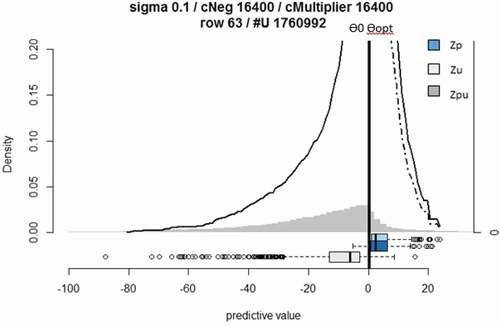
Table 2. Confusion matrices for high severity Maize Lethal Necrosis (MLN) classification using the biased support vectors machine (BSVM) classifier at Ө₀ and Ө_opt thresholds. The + Prediction row of the table corresponds to samples which predicted to be positive (+Pred./high severity MLN). Correctly predicted under +Test (high severity MLN test set) and called the true positives (TP). Inaccurately classified under -Test (low severity MLN test set) and were called the false positives (FP). Similarly, the second row contains the predicted negatives (-Pred./low severity MLN predicts) with true negatives and false negatives (FN). Low severity MLN correctly predicted under -Test (low severity MLN test set) were called the true negatives. Inaccurately classified under +Test (high severity MLN test set) were called the false negatives (FN)

Ө0					Өopt
	+Test	-Test	SUM	UA (%)		+Test	-Test	SUM	UA (%)
+ Pred.	(TP)218	(FP)40	258	84	+ Pred.	(TP)218	(FP)22	240	91
- Pred.	(FN)1	(TN)658	659	100	- Pred.	(FN)1	(TN)676	677	100
SUM	219	698	917		SUM	219	698	917
PA (%)	100	94			PA (%)	100	97
OA (%)	96				OA (%)	97
AUC (*100)	99				AUC (*100)	99
K (*100)	88				K (*100)	93

The OA at Ө₀ and Ө_opt for classifying high severity MLN was 96%, K = 0.88 and 97%, K = 0.93, respectively. At Ө_opt, the UA increased 7% which was a result of lower commission or lower false-positive rate. Similarly, PA at positive test set remained unchanged which means the true positive rate was not reduced. Since it was not easy to determine an optimal threshold, visual inspection was performed too. Finally, Ө_opt was chosen because of its less false-positive rate (Mack et al. 2014). The result of the high severity MLN classification based on BSVM classifier is displayed in Figure 6.

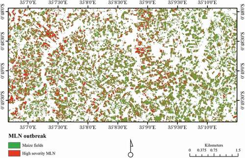
Figure 6. Classification of high severity Maize Lethal Necrosis (MLN) fields using biased support vectors machine (BSVM) classifier and RapidEye data (January 2015).

The classification of the maize field at the long rainy season was challenging due to insufficient (only maize fields) ground truth samples. BSVM was chosen to classify maize fields on L8 imagery at long rainy season. It is important to note that a random sampling approach on the whole training dataset could be used to build unlabelled training samples. In this study, the manual U training sample selection was conducted to build up more representative U training samples. BSVM classification’s histogram (Figure 7) showed high confusion between P and U classes and the Zu and Zp did not show a better separation among the classes. A very tiny break was detected at the Ө_opt (0.93) of diagnostic histogram as presented in Figure 7. The confusion matrices and diagnostic plot indicated that the large part of the Zu samples was located at low z-values and some (i.e. 26) of the unlabelled samples located at Z ≥ 0. This indicates that unlabelled samples were located wrongly where the optimal decision (positive) should be. Practically, a high number of U samples at the P region can indicate the negative effect of imbalanced training samples, which is expected with OCC classifiers. Tax (2002) and Dreiseitl et al. (2010) discussed the outliers issue in detail which is out of the boundary of this work. This misclassification was reduced by choosing Ө_opt during manual interpretation and thresholding. Our study showed that 31% of the maize fields in Bomet were under continuous cropping system (Figure 8).

Figure 7. Biased support vectors machine (BSVM) classification diagnostic plot for mapping maize fields in August 2015 using Landsat 8 data. Zp: distribution of positive prediction, Zu: distribution of unlabelled predictions, Zpu: density histogram of the predicted image.

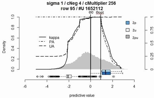
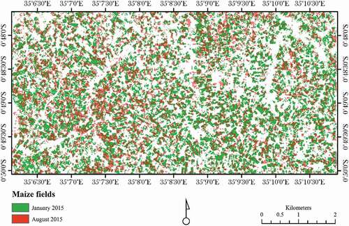
Figure 8. Overlay of classified maize fields in January 2015 and August 2015 obtained using random forest and biased support vectors (BSVM), respectively.

Next step, BSVM classifier was used to classify mono and intercropping maize system in the study area. Figure 9 presents the diagnostic plot out of a balanced P and U training samples. This resulted to an OA of 85% at Ө₀. However, the balanced training samples resulted in a high OA, but analyses of diagnostic plot indicated that 26% of pixels were misclassified at an optimal side for the classified pixels. Notwithstanding, the imbalanced training sample resulted in a lower density region between P and U classes. However, 33% of the unlabelled samples were misclassified. This indicates that imbalanced (Larger U) training samples reached a better separation but also more confusion. Classification with imbalanced P and U training samples resulted with lower OA accuracy of 70% at Ө₀ (Figure 11). In addition, visualized raster showed that at Ө_opt a lot of salt and pepper effects were produced (Figures 10 and 12). After different threshold setting and visual inspection, the threshold 0.4 to 0.5 showed acceptable accuracy. In an optimal situation, larger P and U training samples can cover more complete spectral ranges and consequently the confusion between P and U should be reduced (Khan & Madden, 2014). Bigger training samples here have increased the computational cost. Consequently, the model with smaller but balanced taring samples was chosen to reduce the misclassifications.

Figure 9. Biased support vectors machine (BSVM) classification diagnostic plot trained with balanced samples for mapping maize mono and intercropping systems. Zp: distribution of positive prediction, Zu: distribution of unlabelled predictions, Zpu: density histogram of the predicted image.

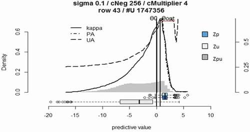
Figure 10. Maize mono and intercropping systems mapped during the high rainy season (western side of Bomet, Kenya).

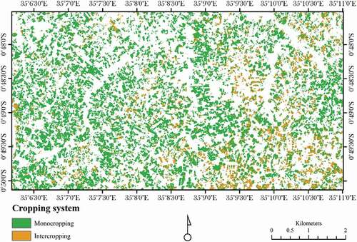
Figure 11. Biased support vectors machine (BSVM) classification diagnostic plot trained with imbalanced samples for mapping maize mono and intercropping systems.

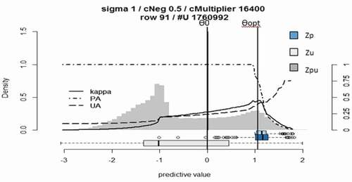
Figure 12. Maize mono- and intercropping systems mapped during the low rainy season (eastern side of Bomet, Kenya).

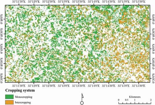
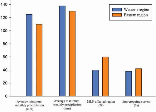
The average-rainfall analysis showed that towards the eastern side of the study area, the precipitation decreased gradually. Whereas, 26% of the study area with relatively higher average rainfalls was under maize intercropping system (Figure 10). At the same period, in the region with lower rainfall, 45% of farmers performed maize intercropping system (Figure 12). Further, our results showed that 60% of high severity MLN occurred at region with lower rainfall (Makone, 2014). Figure 13 presents high severity MLN occurrences, intercropping system, and average rainfall at the western and eastern sides of the study area.

Figure 13. Comparison of western and eastern regions of the study area for precipitation, high severity Maize Lethal Necrosis (MLN), and maize intercropping distribution.

To date, several questions remain unanswered. There is a raising concern about the effectiveness of crop rotation to control MLN outbreak especially in those regions with traditional small-size fields and absence of real cropping calendar. This is particularly important to be investigated that in which extends “long term” crop rotation can be effective to control MLN outbreak in a heterogeneous small-size farming system. Furthermore, distribution of mono and intercropping systems under different rainfall levels revealed that the intercropping system was more common at regions with lower rainfall. The results confirmed that uncertainties in rainfall patterns have encouraged intercropping system in the low rainfall region.

5. Conclusions

This study utilized medium and high spatial resolutions optical (i.e. L8 and RE, respectively), and SAR (i.e. S1, SRTM DEM) datasets towards a better understanding of maize cropping system and high severity MLN occurrences in heterogeneous landscape in Bomet county, Kenya.

Using representative training samples and balanced classes in RF, a LULC map with OA of 89.63% was achieved. We have found a high correlation between maize fields’ NDVI at the adjacent maize development phases such as tasselling and maturation in the same cropping season. The correlation between maize fields’ NDVI in June 2015 and overlapped area at 2014 was only 0.39 which can imply the effect of MLN outbreak on maize crop in the region. Classification of maize fields during long rainy season using L8 imagery and BSVM classifier have been successfully performed. In contrast, RF classifier did not show any outstanding performance with only two classes (i.e. maize and non-maize). This indicates that in the presence of only one known class as training sample, OCC classifiers performed better comparing to RF, which is known as a multi-class classifier.

Classifying high severity MLN and also maize cropping systems (mono and intercropping) using BSVM, performed successfully even the results showed a high confusion rate. Investigating the high severity MLN distribution under different rainfall levels indicated a relatively higher MLN-infected area under lower rainfalls. At the same time, more farmers tended to practice intercropping at lower rainfall levels.

To have a better understanding of ecological variables’ influence on MLN occurrences, further studies should be performed utilizing long term, constant, and accurate data collection methods. In other words, it is important to analyse MLN outbreak trends from the initial year of observation to a longer period to provide a better understanding of MLN occurrences and distribution. Further studies are certainly required to determine presence/absence, alternative hosts, vectors, seasonality of viruses like MCMV and SCMV, and other related ecological factors causing MLN specifically in East Africa. Overall, it will be important to investigate the role of climate change on MLN outbreak to get a better understanding of its effect on food security in Africa.

Acknowledgments

We appreciate the Deutsche Gesellschaft für Internationale Zusammenarbeit (GIZ) for funding of the project “Better implementation of crop season breaks for management of Maize Lethal Necrosis Virus in East Africa – Can remote sensing be an option?” Also, RapidEye Science Archive for the freely available satellite data. We are grateful to Julius-Maximilians-University Würzburg, and our appreciation also extends to the International Centre of Insect Physiology and Ecology (icipe) for helping in identifying maize lethal necrosis (MLN) and its severity as well as field data collection.

Disclosure statement

No potential conflict of interest was reported by the authors.

Additional information

Funding

This work was supported by the Deutsche Gesellschaft für Internationale Zusammenarbeit.

References

- Bannari, A., Morin, D., Bonn, F., & Huete, A. (1995). A review of vegetation indices. Remote Sensing Reviews, 13(1–2), 95–120. https://www.tandfonline.com/doi/abs/10.1080/02757259509532298.
- Braidwood, L., D. F. Quito-Avila, D. Cabanas, A. Bressan, A. Wangai and D. C. Baulcombe (2018) “Maize chlorotic mottle virus exhibits low divergence between differentiated regional sub-populations.” Scientific reports 8, 1173 DOI: https://doi.org/10.1038/s41598-018-19607-4.10.1038/s41598-018-19607-4.
- Braun, A., & Hochschild, V. (2015). Combining SAR and optical data for environmental assessments around refugee camps. GI_Forum, 2015 (1), 424–433. doi: https://doi.org/10.1553/giscience2015s424.
- Breiman, L. J. M. L. (1996). Bagging predictors. 24(2), 123–140. https://doi.org/https://doi.org/10.1007/BF00058655.
- Bryan, E., Ringler, C., Okoba, B., Roncoli, C., Silvestri, S., & Herrero, M. (2013). Adapting agriculture to climate change in Kenya: Household strategies and determinants. Journal of Environmental Management, 114, 26–35. https://doi.org/https://doi.org/10.1016/j.jenvman.2012.10.036
- Conrad, C., Colditz, R. R., Dech, S., Klein, D., & Vlek, P. L. (2011). Temporal segmentation of MODIS time series for improving crop classification in Central Asian irrigation systems. International Journal of Remote Sensing, 32(23), 8763–8778. https://doi.org/https://doi.org/10.1080/01431161.2010.550647.
- Cutler, D. R., Edwards, T. C., Beard, K. H., Cutler, A., Hess, K. T., Gibson, J., & Lawler, J. J. (2007). Random forests for classification in ecology. Ecology, 88(11), 2783–2792. https://doi.org/https://doi.org/10.1890/07-0539.1
- Dreiseitl, S., Osl, M., Scheibböck, C., & Binder, M. (2010). Outlier detection with one-class SVMs: An application to melanoma prognosis. In AMIA Annual Symposium Proceedings, American Medical Informatics Association.
- Forkuor, G., Conrad, C., Thiel, M., Landmann, T., & Barry, B. J. C. (2015). Evaluating the sequential masking classification approach for improving crop discrimination in the Sudanian Savanna of West Africa. Computers and Electronics in Agriculture.118, 380–389.
- Forkuor, G., Conrad, C., Thiel, M., Ullmann, T., & Zoungrana, E. (2014). Integration of optical and synthetic aperture Radar imagery for improving crop mapping in Northwestern Benin, West Africa. Remote Sensing, 6(7), 6472–6499. https://doi.org/https://doi.org/10.3390/rs6076472.
- Hassan, R. M. (1996). Planting strategies of maize farmers in Kenya: A simultaneous equations analysis in the presence of discrete dependent variables. Agricultural Economics, 15(2), 137–149. https://doi.org/https://doi.org/10.1016/S0169-5150(96)01194-2.
- Heinl, M., Walde, J., Tappeiner, G., & Tappeiner, U. (2009). Classifiers vs. input variables—The drivers in image classification for land cover mapping. International Journal of Applied Earth Observation and Geoinformation, 11(6), 423–430. https://doi.org/https://doi.org/10.1016/j.jag.2009.08.002.
- Horning, N. (2010). Random Forests: An algorithm for image classification and generation of continuous fields data sets. In Proceedings of the International Conference on Geoinformatics for Spatial Infrastructure Development in Earth and Allied Sciences. http://wgrass.media.osaka-cu.ac.jp/gisideas10/papers/04aa1f4a8beb619e7fe711c29b7b.pdf.
- Ianninia, L., Molijn, R., & Hanssen, R. (2013). Integration of multispectral and C-band SAR data for crop classification. In SPIE Remote Sensing, International Society for Optics and Photonics. Remote Sensing for Agriculture, Ecosystems, and Hydrology XV.
- Indexmundi. (2019). Kenya corn imports by year. https://www.indexmundi.com/agriculture/?country=ke&commodity=corn&graph=imports.
- Khan, S. S., & Madden, M. G. J. T. K. E. R. (2014). One-class classification: Taxonomy of study and review of techniques. 29(3), 345–374. The Knowledge Engineering Review, 1–24. https://doi.org/https://doi.org/10.1017/S026988891300043X.
- Kimani, S., Macharia, J., Gachengo, C., Palm, C., & Delve, R. (2004). Maize production in the central Kenya Highlands using cattle manures combined with modest amounts of mineral fertilizer. Uganda Journal of Agricultural Sciences, 9(1), 480–490. https://www.ajol.info/index.php/ujas/article/viewFile/134989/124493.
- Kiruwa, F. H., Feyissa, T., & Ndakidemi, P. A. J. A. J. O. M. R. (2016). Insights of maize lethal necrotic disease: A major constraint to maize production in East Africa. African Journal of Microbiology Research .10(9), 271–279. https://doi.org/10.5897/AJMR2015.7534 .
- Kross, A., McNairn, H., Lapen, D., Sunohara, M., & Champagne, C. (2015). Assessment of RapidEye vegetation indices for estimation of leaf area index and biomass in corn and soybean crops. International Journal of Applied Earth Observation and Geoinformation, 34, 235–248. https://doi.org/https://doi.org/10.1016/j.jag.2014.08.002.
- Kuhn, M. (2007). Variable importance using the caret package. http://btr0x2.rz.uni-bayreuth.de/math/statlib/R/CRAN/doc/vignettes/caret/caretVarImp.pdf.
- Mack, B., R. Roscher and B. J. R. S. Waske (2014). “Can i trust my one-class classification?”. 6(9): 8779–8802.
- Mack, B., & Waske, B. J. R. S. L. (2017). In-depth comparisons of MaxEnt, biased SVM and one-class SVM for one-class classification of remote sensing data. Remote sensing letters. 8(3), 290–299. https://doi.org/https://doi.org/10.1080/2150704X.2016.1265689.
- Mack, B. M. (2017). Applied one-class classification of remote sensing data. https://refubium.fu-berlin.de/handle/fub188/6686.
- Mahuku, G., Lockhart, B. E., Wanjala, B., Jones, M. W., Kimunye, J. N., Stewart, L. R., Cassone, B. J., Sevgan, S., Nyasani, J. O., & Kusia, E. (2015). Maize lethal necrosis (MLN), an emerging threat to maize-based food security in sub-Saharan Africa. Phytopathology, 105(7), 956–965. https://doi.org/https://doi.org/10.1094/PHYTO-12-14-0367-FI
- Makone, S. M. (2014). Extent To Which Maize Lethal Necrosis Disease Affects Maize Yield: A Case Of Kisii County. Kisii University.
- Marenya, P. P., Erenstein, O., Prasanna, B., Makumbi, D., Jumbo, M., & Beyene, Y. (2018). Maize lethal necrosis disease: Evaluating agronomic and genetic control strategies for Ethiopia and Kenya. Agricultural Systems. 162, 220–228. https://doi.org/https://doi.org/10.1016/j.agsy.2018.01.016.
- Namikoye, E., Kariuki, G., Kinyua, Z., Githendu, M., Kasina, M. J. E. A. A., & Journal, F. (2017). Cropping system intensification as a management method against vectors of viruses causing Maize Lethal Necrosis Disease in Kenya. East African Agricultural and Forestry . 82(2–4), 246–260. https://doi.org/https://doi.org/10.1080/00128325.2018.1456298.
- Nault, L., Styer, W., Coffey, M., Gordon, D., Negi, L., & Niblett, C. (1978). Transmission of maize chlorotic mottle virus by chrysomelid beetles. Phytopathology, 68(7), 1071–1074. https://www.apsnet.org/publications/phytopathology/backissues/Documents/1978Articles/Phyto68n07_1071.PDF.
- Nyoro, J. K., Kirimi, L., & Jayne, T. S. (2004). Competitiveness of Kenyan and Ugandan maize production: Challenges for the future. International Development Collaborative Working Papers KE-TEGEMEO-WP-10, Department of Agricultural Economics, Michigan State University.
- Ochieng, L. A., Mathenge, P., & Muasya, R. J. A. J. O. F., Agriculture, Nutrition and Development. (2011). A survey of on-farm seed production practices of sorghum (Sorghum bicolor L. Moench) in Bomet district of Kenya. African Journal of Food, Agriculture, Nutrition and Development. 11(5), 5232–5253. https://www.ajol.info/index.php/ajfand/article/view/70448.
- Olwande, J., Sikei, G., & Mathenge, M. (2009). Agricultural technology adoption: A panel analysis of smallholder farmers’ fertilizer use in Kenya. Center of Evaluation for Global Action.
- Oshiro, T. M., Perez, P. S., & Baranauskas, J. A. (2012). How many trees in a random forest? In International Workshop on Machine Learning and Data Mining in Pattern Recognition, Springer.
- Osunga, M., Mutua, F., & Mugo, R. J. J. O. G. (2017). Spatial modelling of Maize Lethal Necrosis Disease in Bomet County, Kenya. Journal of Geosciences and Geomatics. 5(5), 251–258.doi:https://doi.org/10.12691/jgg-5-5-4
- Ozdarici, A., & Akyurek, Z. (2010). A comparison of SAR filtering techniques on agricultural area identification. In ASPRS 2010 Annual Conference. (pp. 26–30). San Diego. Retrieved from http://www.asprs.org/wp-content/uploads/2013/08/Ozdarici.pdf
- Richter, R., & Schläpfer, D. (2005). Atmospheric/topographic correction for satellite imagery (DLR report DLR-IB: 565–501). DLR - German Aerospace Center. https://www.dlr.de/eoc/Portaldata/60/Resources/dokumente/5_tech_mod/atcor3_manual_2012.pdf.
- Stewart, L. R., Willie, K., Wijeratne, S., Redinbaugh, M. G., Massawe, D., Niblett, C. L., Kiggundu, A., & Asiimwe, T. (2017). Johnsongrass mosaic virus contributes to Maize Lethal Necrosis in East Africa (Plant Disease: The American Phytopathological Society. PDIS-01-17-0136-RE). https://doi.org/https://doi.org/10.1094/PDIS-01-17-0136-RE
- Tax, D. M. J. (2002). One-class classification: Concept learning in the absence of counter-examples. https://repository.tudelft.nl/islandora/object/uuid:e588fc3e-7503-4013-9b6a-73c7b7f6b173/datastream/OBJ/download
- Whiteside, T. G., Boggs, G. S., & Maier, S. W. (2011). Comparing object-based and pixel-based classifications for mapping savannas. International Journal of Applied Earth Observation and Geoinformation, 13(6), 884–893. https://doi.org/https://doi.org/10.1016/j.jag.2011.06.008.
- Zillmann, E., & Weichelt, H. (2014). Crop identification by means of seasonal statistics of RapidEye time series. Agro-geoinformatics (Agro-geoinformatics 2014), Third International Conference on, IEEE.