Extending the concept of entropy-negentropy for the assessment of ecological dominance and diversity at alpha, beta and gamma levels

ABSTRACT

Several measures of ecological diversity have been defined at alpha, beta, and gamma levels and less attention has been paid to characterise their ecological dominance. In this paper, we extend the concept of negative entropy (negentropy) for the measurement of ecological dominance and diversity at the three hierarchical levels of community characterization. Negentropy is a measure of energy, and gives a convex curve for binary negentropy function, whereas Shannon’s entropy gives a typical concave curve. Similarly, we have defined indices for Simpson’s and Brillouin’s dominance functions at alpha, beta and gamma levels. The results of diversity indices followed a trend for different sites as: Harike > Beas > Goindwal Sahib, while trend obtained for dominance is Goindwal Sahib > Beas > Harike. The pooled results of both indicated that Harike showed maximum ecological information by the application of Shannon’s diversity and Simpson’s inverse diversity, while results of Simpson’s diversity remain same for all sites.

KEYWORDS:

• Entropy
• negentropy
• dominance
• Shannon’s diversity
• Simpson’s dominance
• Brillouin’s information
• binary entropy plot
• beta diversity
• community
• phytosociology

Introduction

The vital objective of ecology is to delineate the mechanisms which are essential for the sustainability of ecosystems (Tilman et al., 2014). Any damage to biodiversity destroys the functionality of ecosystems, and in severe circumstances leads to the mass extinction of species and the loss of whole ecosystems (Dunne & Williams, 2009). Biodiversity in its widest sense is defined as the variety of life forms at different levels, ranging from the organismic levels to the species (DeLong, 1996; Pandita et al., 2019). By applying diversity indices, we can compare diverse spatial sites and temporal periods etc. (Daly et al., 2018). These measures are thus important tools for ecological monitoring and conservation, and to deal with any biodiversity calamity (Morris et al., 2014). Ecological dominance and diversity are extensively used community features at alpha, beta and gamma levels (Thukral et al., 2019), and these diversity measures are widely applied in the ecology from the last few decades (Semeniuk &, Cresswell 2013). Some of the measures used for the determination of community diversity are Shannon’s entropy (Shannon-Weiner’s index) (Shannon, 1948), Simpson’s index (Simpson, 1949), Brillouin’s index (Brillouin, 1953, 1962), Renyi’s entropy (Renyi, 1961), Berger-Parker’s index (Berger & Parker, 1970) etc.

Dominance

Common indices used for the measurement of dominance are Simpson’s index, Berger-Parker index and McIntosh index.

Entropy as a measure of diversity

Shannon’s entropy (H’) is one of the most preferred measures of diversity, and is given by the equation,

$H^{\prime }=-\sum _{i=1}^K{p}_{i}ln{p}_i=-\hspace{0.17em}\sum i=1K\hspace{0.17em}\frac{n_i}{N}ln\frac{n_i}{N}$

where p_i is the probability of occurrence of a species, and K is the number of species in a community.

Simpson’s index of diversity (C’) and Simpson’s inverse index of diversity (D’) are represented by the equation as:

$C{ }^{\mathrm{\prime }}=1-\sum _{i=1}^K{p}_i^2$

$D^{\prime }=\frac{1}{{\sum }_{i=1}^K{p}_i^2}$

Simpson’s index of dominance (C) is also known as Simpson’s index with replacement and is used if the sample is quite large.

$C=\sum _{i=1}^K{p}_i^2={\left(\frac{n_i}{N}\right)}^2$

where, p_i is probability of occurrence of a species in the community, K is the number of species and n_i is the number of individuals of the i^th species, and N is the total number of individuals of all the species. The maximum value of Simpson’s index for a single species community is 1, and the minimum value for an evenly distributed species is (1/K)². If the sample size is small, Simpson’s index of dominance without replacement is used,

$C=\frac{{\sum }_{i=1}^K{n}_i\left(n_i-1\right)}{N\left(N-1\right)}$

Berger-Parker index of dominance (D_BP) is the proportion of number of individuals of the dominant species (n_D) to the total number of individuals of all the species (N),

$D_{BP}=\frac{n_D}{N}$

For a single species community, the value of Berger-Parker dominance index is 1 (maximum), and for an evenly distributed community, the value is 1/K, where K is the number of species. McIntosh’s U is a dominance index,

$U_{McIntosh}=\sqrt{\sum _1^K{p}_i^2}$

where pi represents the proportional number of individuals of different species present in a community.

Relation between entropy and negentopy

The concept of negative entropy was given by Schrödinger (1944), and later elaborated by Brillouin (1953), who introduced the term negentropy. Among all the probability distributions, normal distribution has the maximum entropy, negentropy is always non-negative (Quarati et al., 2016). The relation between entropy (S) and negentropy (J) of a system is given by the equation,

$J=S_{max}-S$

where, S_max is the maximum entropy possible. This also implies that sum of entropy and negentropy of a system is equal to the theoretical maximum entropy, i.e.,

$J+S=S_{max}$

If entropy measures order in a system, negentropy measures the disorder. Negentropy may also be treated as the energy not utilised (E’) by the system and available for work, i.e., $J=E^{\prime }$. Because, maximum order and maximum disorder are equal, we have$S_{max}=E{ }_{max}^{\prime }$. Thus, in terms of energy, we can rewrite the entropy equation as,

$E^{\prime }+S=E{ }_{max}^{\prime }$

In ecological systems, dominance and diversity characterize the numerical structure of different species. Shannon’s index of diversity (H’) is a measure of entropy. Since a community with even distribution of species has the maximum entropy (H’_max), we can extend the concept of negentropy (E’) to the study of ecological dominance:

$E^{\prime }=H{ }_{max}^{\prime }-H{ }^{\mathrm{\prime }}$

Diversity and dominance are two inseparable aspects of biological community studies, and are generally studied together. However, diversity indices are more common in literature (Kumar et al., 2017; Parkash & Thukral, 2010; Sarangal et al., 2012; Thukral, 2017). Further, community characterization at β and γ levels is generally restricted to diversity only, some of the indices used are given in (Table 1). The present work, therefore, focuses on defining new ecological dominance indices at alpha level, and extending the concept of ecological dominance at β and γ levels.

Table 1. Some beta diversity indices from PAST software (Hammer et al., 2001).

Whittaker (1960)	$\frac{K}{\alpha }-1$
Harrison et al. (1992)	$\frac{\frac{K}{\alpha }-1}{N-1}$
Cody (1975)	$\frac{g\left(S\right)+l\left(S\right)}{2}$
Wilson-Shmida (1984)	$\frac{g\left(S\right)+l\left(S\right)}{2\alpha }$
Mourelle and Ezcurra (1997)	$\frac{g\left(S\right)+l\left(S\right)}{2\alpha \left(N-1\right)}$
Harrison et al. (1992)	$\frac{\frac{K}{{\alpha }_{max}}-1}{N-1}$
Williams (1996)	$1-\frac{{\alpha }_{max}}{K}$

Methods

Dominance and diversity

Drawn from the relation between entropy and negentropy, we can write the relationships between ecological dominance and diversity for some known diversity and dominance indices as given in (Table 2).

Table 2. Negentropy measures of four common indices used in ecological diversity and dominance.

Measure	Entropy as Diversity	Negentropy as Dominance	Maximum entropy
Shannon’s	$H{ }^{\mathrm{\prime }}=-\sum _{i=1}^K{p}_{i}ln{p}_i$	$E{ }^{\mathrm{\prime }}=lnK-\sum _{i=1}^K{p}_{i}ln{p}_i$	$lnK$
Simpson’s	$C{ }^{\mathrm{\prime }}=1-\sum _{i=1}^K{p}_i^2$	$C=\sum _{i=1}^K{p}_i^2$	1
Simpson’s inverse	$D^{\prime }=\frac{1}{{\sum }_{i=1}^K{p}_i^2}$	$D=K-\frac{1}{{\sum }_{i=1}^K{p}_i^2}$	K
Brillouin’s	$H=ln\frac{N!}{n_1!n_2!\dots n_K!}$	$E=\frac{lnN!}{N}-ln\frac{N!}{n_1!n_2!\dots n_K!}$	$\frac{lnN!}{N}$

Levels of diversity

Community diversity can be studied at three levels, alpha (α), beta (β) and gamma (γ). Alpha diversity is defined as the diversity of a single sample or community. For a landscape consisting of M communities, Shannon’s α diversity, $\alpha \left(H{ }^{\mathrm{\prime }}\right)$, is the average community diversity:

$\alpha \left(H{ }^{\mathrm{\prime }}\right)=\frac{1}{M}\sum _{j=1}^{M}H{ }_j^{\prime }$

Similarly, Simpson’s α diversity of a landscape α(C’), Simpson’s inverse alpha diversity α(D’), and Brillouin’s α diversity α(H) consisting of M communities may be defined, respectively, as,

$\alpha \left(C^{\prime }\right)=\frac{1}{M}\sum _{j=1}^{M}C{ }_j^{\prime }$

$\alpha \left(D^{\prime }\right)=\frac{1}{M}\sum _{j=1}^{M}D{ }_j^{\prime }$

$\alpha \left(H\right)=\frac{1}{M}\sum _{j=1}^M{H}_j$

Gamma diversity is the diversity of the landscape consisting of two or more communities considering that the landscape is a single community. The relationship between α, β and γ diversities may be described using additive or multiplicative models (Whittaker, 1972). The additive model gives the value of γ diversity as,

$\gamma =\alpha +\beta$

where, β diversity is the difference of diversities at two levels (γ-α). The entropies at α and γ levels cannot be negative, but their difference, mentioned in this manuscript as (β_add) diversity, can be positive, negative or zero. Using the additive model, Shannon’s β diversity, β(H’) of a landscape consisting of M communities, may also be written as,

${\beta }_{add.}\left(H{ }^{\mathrm{\prime }}\right)=\gamma \left(H{ }^{\mathrm{\prime }}\right)-\alpha \left(H{ }^{\mathrm{\prime }}\right)$

where, α(H’), β(H’) and γ(H’) are Shannon’s additive α, β, and γ diversities, respectively. The multiplicative model is based on effective number of species in a community (β_mult.) i.e., e^H’. For α, β and γ Shannon’s entropies, the multiplicative beta diversity is.

$e^{\gamma }=e^{\alpha }.e^{\hspace{0.17em}}$

where $e^{\hspace{0.17em}}$ is ratio of two diversities and is given by $e^{\gamma }/e^{\alpha }$. Shannon’s multiplicative model is also written as:

${\beta }_{mult.}\left(H{ }^{\mathrm{\prime }}\right)=\frac{\gamma \left(H{ }^{\mathrm{\prime }}\right)}{\alpha \left(H{ }^{\mathrm{\prime }}\right)}$

where, α(H’), β(H’) and γ(H’) are the exponential functions, e^α, e^β and e^γ of the three diversities respectively. Similarly, the additive model for Simpson’s β diversity, β(C’), Simpson’s inverse β diversity, β(D’), Brillouin’s β diversity, β(H) of a landscape consisting of M communities, may be defined, respectively, as,

${\beta }_{add.}\left(C{ }^{\mathrm{\prime }}\right)=\gamma \left(C{ }^{\mathrm{\prime }}\right)-\alpha \left(C{ }^{\mathrm{\prime }}\right)$

${\beta }_{add.}\left(D{ }^{\mathrm{\prime }}\right)=\gamma \left(D{ }^{\mathrm{\prime }}\right)-\alpha \left(D{ }^{\mathrm{\prime }}\right)$

${\beta }_{add.}\left(H\right)=\gamma \left(H\right)-\alpha \left(H\right)$

We have similarly defined the dominance equations at α, β and γ levels. In this paper we have used only the additive models of entropy and negentropy for diversity and dominance measurements. We have used our models in different communities under four hypothetical situations:

1. Each community having one different species with equal number of individuals of each species.

2. Only one species having equal number of individuals in all the communities.

3. Five different species, each having different numbers of individuals.

4. Communities having different number of species, each species having different number of individuals.

Results

Derivation of negentropic indices of dominance

In this paper, we extend the concept of negentropy to the study of community dominance and diversity at alpha, beta and gamma levels. We have used Euler’s constant (e) as the base for logarithm to give entropy or negentropy in nats for Shannon’s and Brillouin’s indices. Alternatively, the logarithms could be used with base 2 (units as bits or Shannon’s), or base 10 (units as decits). Using Shannon’s entropy, we define negentropic index of dominance (E’), as follows:

$E^{\prime }=H{ }_{max}^{\prime }-H{ }^{\mathrm{\prime }}$

where, E’ is the negentropy, H’ is the entropy or diversity, and H’_max is the theoretical maximum entropy of the community if all the species are evenly distributed. If a community consists of K species, maximum Shannon’s diversity is given as ${H_{max}}^{\prime }=lnK$, therefore,

$E^{\prime }=lnK-H^{\prime }$

We have given the negentropies derived as measures of dominance in (Table 2). For a landscape consisting of M communities, α dominance may be defined as the average community dominance:

$\alpha \left(E^{\prime }\right)=\frac{1}{M}\sum _{j=1}^{M}E{ }_j^{\prime }$

where E’_j is negentropy of the j^th community. Negentropic β dominance, β(E’) of a landscape consisting of M communities, may be defined as,

${\beta }_{add.}\left(E^{\prime }\right)=\gamma \left(E^{\prime }\right)-\alpha \left(E^{\prime }\right)$

where γ(E’) is negentropic dominance index of the landscape. Like Shannon’s entropy, the negentropies, α and γ, are non-negative, but the negentropy ${\beta }_{add.}\left(E^{\prime }\right)$ can be positive, negative or zero, depending on the magnitudes of α and γ negentropies. Negentropies for Simpson’s dominance (C), Simpson’s inverse dominance (D) and Brillouin’s dominance (E) may be defined accordingly at β and γ levels:

${\beta }_{add.}\left(C\right)=\gamma \left(C\right)-\alpha \left(C\right)$

${\beta }_{add.}\left(D\right)=\gamma \left(D\right)-\alpha \left(D\right)$

${\beta }_{add.}\left(E\right)=\gamma \left(E\right)-\alpha \left(E\right).$

Binary entropy and negentropy functions

Binary entropy function is the Shannon’s entropy of a 2-class variable, with the probabilities of the two states being p and q, such that q = 1 – p (Guedes et al., 2016). The entropy of this variable is given as,

$H{ }^{\mathrm{\prime }}=-(plnp+qlnq)$

Binary entropy was calculated for different values of p varying from 0 to 1, and a plot between entropy (H’) and probability of the first class (p) is called binary entropy function plot (Figure 1). We can extend the binary entropy function to binary negentropy function using the relation,

$E^{\prime }=ln2-(plnp+qlnq).$

Figure 1. Binary information plots for Shannon’s entropy and negentropy.

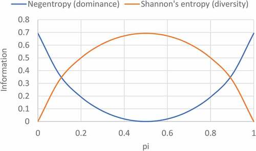
A plot between the negentropy (E’) and the probability (p) may be called binary negentropy function. Binary entropy plot between probability and Shannon’s entropy gives a typical concave curve, whereas binary negentropy plot gives a convex curve (Figure 1). Binary entropy plot may also be called binary information plot in a wider sense of usage. (Figure 1) depicts that in the initial phase when Shannon’s entropy increases then negentropy or dominance decreases, but at the end Shannon’s entropy declines, while negentropy or dominance increases. In information theory, entropy is regarded as a measure of uncertainty. To put it instinctively, suppose pi = 0, the event is assured never happen, and thus there is no ambiguity at all, leading to entropy of zero. If pi = 1, the result is again definite; consequently, the entropy is zero as well. In case of pi = ½, the results indicate that ambiguity is maximum, if one were to place a fair bet on the outcome in this case, there is no benefit to be added with earlier gen of the probabilities. In this case, the entropy is highest at value of 1 bit. Intermediary values falls between these cases. For example, if pi = ¼, there is tranquil a measure of ambiguity on the result, but one can still foresee the result appropriately more frequently than not, so the ambiguity measure or entropy, is less than 1 full bit. (Figure 2) gives binary information plot between the information and probability of a two-class variable for Simpson’s dominance (C) and diversity (C’).

$C=p^2+q^2$

$C{ }^{\mathrm{\prime }}=1-\left(p^2+q^2\right)$

Figure 2. Binary information plots for Simpson’s dominance and diversity.

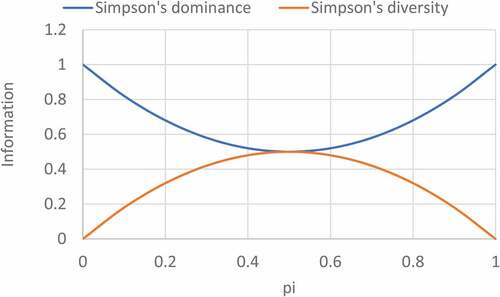
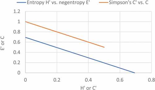
Simpson’s C gives a convex energy curve, like that of Shannon’s negentropy, whereas Simpson’s C’ gives a concave information curve, like Shannon’s entropy. (Figure 3) shows that entropy and negentropy; and diversity and dominance are negatively linearly correlated, and thus can be used as complementary community attributes. The diversity decreases with the increase of dominance as shown by (Figure 3). Dominance will be maximum when diversity approaches towards unity, although diversity of community consisting of more than one species will be maximum if all the species have an equal number of individuals. The negentropy characterising with organized actions of the control subject eradicates ambiguity (entropy) and it is the quantitative information measure. The removing of the ambiguity is articulated through the alterations of conditions that executed on the system and its entropy. The protective of system structure strength is a fight against entropy, which reveals aging process in technical systems. The requisite to upsurge the negentropy is the requirement to recompense the entropy as much as the entropy can be reduced itself. The problem solution of the removal ambiguity will permit to plan actions to decrease entropy established on the negentropy principle of Brillouin’s information about the structural system alterations. A negative change in entropy refers to increasing orderness thereby increasing the diversity of community. The possibility of such an occurrence seems to break the laws of thermodynamics, but that law refers to an isolated system, not each individual part of the system. For example, when our cells convert ADP and phosphate into ATP, the product is more ordered than the reaction and a negative change in entropy has happened. The entire system, however, has become more disordered because the cell has to convert glucose, an ordered compound, into water and carbon dioxide. The entire system, therefore, obeys the second law of thermodynamics (Martin et al., 2013).

Figure 3. Negative correlation between binary Shannon’s entropy (H’) and negentropy (E’); and Simpson’s diversity (C’) and dominance (C) .

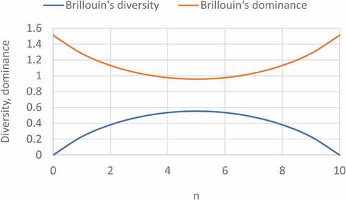
(Figure 4) gives the binary information plot between the probability, and Simpson’s diversity (concave) and dominance (convex) indices. Since Brillouin’s index uses the number of individuals of different species instead of probability, we have plotted binary information function for Brillouin’s diversity and dominance as defined in (Table 2) and (Figure 5), using the number of individuals (n) on a 0–10 scale, instead of probability (0–1). It is seen that Brillouin’s diversity and dominance give typical concave curve for diversity and convex for dominance. From (Figure 5), it was found that if Brillouin’s diversity increases then Brillouin’s dominance decreases and both are inversely related with each other. In initial phase the Brillouin’s diversity was increased but dominance decreases and after that at the end phase Brillouin’s diversity decreases while Brillouin’s dominance increases.

Figure 4. Binary information plots for Simpson’s inverse dominance and diversity.

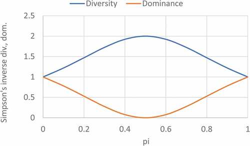
Figure 5. Binary information plots for Brillouin’s dominance and diversity.

In order to understand the behavior of diversity and dominance attributes under different situations, data were created using hypothetical communities (Tables 3–5). (Table 3) presents 5 communities, each community having a unique species not present in any other community. There is an increase in diversity due to Shannon’s, Simpson’s inverse information and Brillouin’s entropies in the pooled community. But as expected, the negentropy-based dominance indices did not change in Shannon’s, Simpson’s inverse and Brillouin’s models.

Table 3. Dominance and diversity indices in five single species communities consisting of different species with equal number of individuals.

	Number of individuals in five α communities (C1 … C5)					γ-Community
Species	C1	C2	C3	C4	C5	C1 … C5
I	10	-	-	-	-	10
II	-	10	-	-	-	10
III	-	-	10	-	-	10
IV	-	-	-	10	-	10
V	-	-	-	-	10	10
Total ind.	10	10	10	10	10	50
No. of Spp.	1	1	1	1	1	5
	Shannon’s diversity, dominance (negentropy)
Div = (H’)	0	0	0	0	0	1.61
Dom = (H’max -H’)	0	0	0	0	0	0
Div + Dom = H’max	0	0	0	0	0	1.61
	Simpson’s diversity, dominance
Div = (1-∑ pi^2)	0	0	0	0	0	0.8
Dom = (∑pi^2)	1	1	1	1	1	0.2
Div + Dom = C’max	1	1	1	1	1	1
	Simpson’s inverse diversity, dominance
Div = (1/∑pi^2)	1	1	1	1	1	5
Dom = (K-1/∑pi^2)	0	0	0	0	0	0
Div + Dom = K	1	1	1	1	1	5
	Brillouin’s diversity, dominance
Div = (H)	0	0	0	0	0	1.46
Dom = (Hmax-H)	1.51	1.51	1.51	1.51	1.51	1.51
Div + Dom = Hmax	1.51	1.51	1.51	1.51	1.51	2.97
	α		γ		βadd. = γ-α
	Shannon’s α, γ, β
Diversity	0		1.61		1.61
Dominance	0		0		0
Div + Dom	0		1.61		1.61
	Simpson’s α, γ, β
Diversity	0		0.8		0.8
Dominance	1		0.2		−0.8
Div + Dom	1		1		0
	Simpson’s inverse α, γ, β
Diversity	1		5		4
Dominance	0		0		0
Div + Dom	1		5		4
	Brillouin’s α, γ, β
Diversity	0		1.46		1.46
Dominance	1.51		1.51		0
Div + Dom	1.51		2.97		1.46

Table 4. Dominance and diversity indices in five single species communities consisting of the same species with equal number of individuals.

	Number of individuals in five α communities (C6 … C10)					γ-Community
Species	C6	C7	C8	C9	C10	C6 … C10
I	10	10	10	10	10	50
II	-	-	-	-	-	-
III	-	-	-	-	-	-
IV	-	-	-	-	-	-
V	-	-	-	-	-	-
Total ind.	10	10	10	10	10	50
No. of Spp.	1	1	1	1	1	1
	Shannon’s diversity, dominance (negentropy)
Div = (H’)	0	0	0	0	0	0
Dom = (H’max -H’)	0	0	0	0	0	0
Div + Dom = H’max	0	0	0	0	0	0
	Simpson’s diversity, dominance
Div = (1-∑ pi^2)	0	0	0	0	0	0
Dom = (∑pi^2)	1	1	1	1	1	1
Div + Dom = C’max	1	1	1	1	1	1
	Simpson’s inverse diversity, dominance
Div = (1/∑pi^2)	1	1	1	1	1	1
Dom = (K-1/∑pi^2)	0	0	0	0	0	0
Div + Dom = K	1	1	1	1	1	1
	Brillouin’s diversity, dominance
Div = (H)	0	0	0	0	0	0
Dom = (Hmax-H)	1.51	1.51	1.51	1.51	1.51	2.97
Div + Dom = Hmax	1.51	1.51	1.51	1.51	1.51	2.97
	α		γ		βadd. = γ-α
	Shannon’s α, γ, β
Diversity	0		0		0
Dominance	0		0		0
Div + Dom	0		0		0
	Simpson’s α, γ, β
Diversity	0		0		0
Dominance	1		1		0
Div + Dom	1		1		0
	Simpson’s inverse α, γ, β
Diversity	1		1		0
Dominance	0		0		0
Div + Dom	1		1		0
	Brillouin’s α, γ, β
Diversity	0		0		0
Dominance	1.51		2.97		1.46
Div + Dom	1.51		2.97		1.46

Table 5. Dominance and diversity indices in five communities consisting of equal number of species with different number of individuals.

	Number of individuals in five α communities (C11 … C15)					γ-Community
Species	C11	C12	C13	C14	C15	C11 … C15
I	2	54	3	51	2	112
II	8	2	23	45	7	85
III	21	1	61	2	12	97
IV	1	27	2	1	34	65
V	5	2	6	61	2	76
Total ind.	37	86	95	160	57	435
No. of Spp.	5	5	5	5	5	5
	Shannon’s diversity, dominance (negentropy)
Div = (H’)	1.18	0.88	0.99	1.17	1.13	1.59
Dom = (H’max – H’)	0.42	0.73	0.62	0.44	0.48	0.02
Div + Dom = H’max	1.61	1.61	1.61	1.61	1.61	1.61
	Simpson’s diversity, dominance
Div = (1-∑pi^2)	0.61	0.51	0.52	0.67	0.58	0.79
Dom = (∑pi^2)	0.39	0.49	0.48	0.33	0.42	0.21
Div + Dom = C’max	1	1	1	1	1	1
	Simpson’s inverse diversity, dominance
Div = (1/∑pi^2)	2.56	2.04	2.08	3.03	2.38	4.76
Dom = (K-1/∑pi^2)	2.44	2.96	2.92	1.97	2.62	0.24
Div + Dom = K	5	5	5	5	5	5
	Brillouin’s diversity, dominance
Div = (H)	1.02	0.81	0.92	1.13	1.02	1.57
Dom =  (Hmax-H)	1.66	2.68	2.67	2.97	2.07	3.51
Div + Dom = Hmax	2.68	3.49	3.59	4.10	3.09	5.08
	α		γ		βadd. = γ-α
			Shannon’s α, γ, β
Diversity	1.07		1.59		0.52
Dominance	0.54		0.02		−0.52
Div + Dom	1.61		1.61		0
	Simpson’s α, γ, β
Diversity	0.58		0.79		0.21
Dominance	0.42		0.21		−0.21
Div + Dom	1		1		0
	Simpson’s inverse α, γ, β
Diversity	2.42		4.76		2.34
Dominance	2.58		0.24		−2.34
Div + Dom	5.00		5.00		0
	Brillouin’s α, γ, β
Diversity	0.98		1.57		0.59
Dominance	2.41		3.51		1.10
Div + Dom	3.39		5.08		1.69

(Table 4) consisting of the same species in individual and pooled communities shows that Shannon’s and Simpson’s inverse indices due to entropy and negentropy do not change in pooled community. If the number of species are equal in all the communities, the sum of β diversity and β dominance is zero for Shannon’s, Simpson’s and Simpson’s inverse indices (Table 5). (Table 6) is an example of the most common situation, where both the number of species and number of individuals per species are different in different communities. The sum of entropy and negentropy for all the dominance and diversity indices is additive.

Table 6. Dominance and diversity indices in five communities consisting of different number of species with different number of individuals.

	Number of individuals in five α communities (C16 … C20)					γ-Community
Species	C16	C17	C18	C19	C20	C16 … C20
I	2	54	3	51	2	112
II	8	2	23	-	7	40
III	21	1	61	-	12	95
IV	1	-	-	-	34	35
V	-	2	-	-	2	4
Total ind.	32	59	87	51	57	286
No. of Spp.	4	4	3	1	5	5
	Shannon’s diversity, dominance (negentropy)
Div = (H’)	0.90	0.38	0.72	0	1.13	1.33
Dom = (H’max – H’)	0.49	1.01	0.38	0	0.48	0.28
Div + Dom = H’max	1.39	1.39	1.10	0	1.61	1.61
	Simpson’s diversity, dominance
Div = (1-∑pi^2)	0.50	0.16	0.43	0	0.58	0.70
Dom = (∑pi^2)	0.50	0.84	0.57	1	0.42	0.30
Div + Dom = C’max	1	1	1	1	1	1
	Simpson’s inverse diversity, dominance
Div = (1/∑pi^2)	2	1.19	1.75	1	2.38	3.33
Dom = (K-1/∑pi^2)	2	2.81	1.25	0	2.62	1.67
Div + Dom = K	4	4	3	1	5	5
	Brillouin’s diversity, dominance
Div = H)	0.78	0.32	0.67	0	1.02	1.29
Dom = (Hmax-H)	1.77	2.81	2.83	2.99	2.07	3.38
Div + Dom = Hmax	2.55	3.13	3.50	2.99	3.09	4.67
	α		γ		βadd. = γ-α
	Shannon’s α, γ, β
Diversity	0.63		1.33		0.70
Dominance	0.47		0.28		−0.19
Div + Dom	1.10		1.61		0.51
	Simpson’s α, γ, β
Diversity	0.65		0.87		0.22
Dominance	0.35		0.13		−0.22
Div + Dom	1		1		0
	Simpson’s inverse α, γ, β
Diversity	1.66		3.33		1.67
Dominance	1.74		1.67		−0.07
Div + Dom	3.4		5		1.6
	Brillouin’s α, γ, β
Diversity	0.56		1.29		0.73
Dominance	2.49		3.38		0.89
Div + Dom	3.05		4.67		1.62

Beta diversity along river Beas, India – A case study

(Table 7) gives number of individuals of species present in the river-side vegetation along river Beas, flowing downstream from Beas 31.51 N, 75.28 E – Goindwal Sahib 31.68 N, 75.13 E (about 36 km) and then to Harike wetland 31.17 N, 75.20 E (about 41 km). The distances between the three sites along the river from Beas to Goindwal Sahib and then to Beas, were 36 km and 41 km, respectively. Harike wetland a man-made lake situated at the confluence of two rivers: Sutlej and Beas, and is Ramsar site. River Beas is a relatively less polluted river and harbors a threatened species of dolphin, Platanista minor. The quadrats of size 100 cm × 100 cm were laid down arbitrarily at each site. The methodology applied was adapted from Kumar et al. (2018). The order of diversity indices used was Harike > Beas > Goindwal Sahib. For dominance, the order was Goindwal Sahib > Beas > Harike. The combined results of diversity and dominance indices showed the trend as Harike > Beas > Goindwal Sahib for Shannon’s diversity and Simpson’s inverse diversity, however, for Simpson’s diversity the value remains constant. For Brillouin’s diversity index of dominance, the trend obtained is as: Harike > Goindwal Sahib > Beas. The results clearly indicate that diversity indices are better in contrast to dominance. Furthermore, the application of both in combination better elucidated the ecological information. (Table 7) shows the method of calculation, and relations among alpha, beta and gamma dominance and diversity indices.

Table 7. Dominance and diversity indices along River Beas downstream from Beas to Harike, India. Data on number of individuals from six quadrats (1 sq. m each) from each community.

	Number of individuals in three α communities				γ-Community
Species	Beas	Goindwal		Harike	Riverine Landscape
Ageratum conyzoides L.	17	5			22
Alternanthera philoxeroides (Mart.) Grisb.	6				6
Ampelopteris prolifera (Retz.) Copel				6	6
Argemone mexicana L.				4	4
Cannabis sativa L.				3	3
Chenopodium ambrosoides L.	5			15	20
Erigeron bonariensis L.		8			8
Fumaria parviflora Lam.				10	10
Oxalis corniculata L.				5	5
Parthenium hysterophorus L.	6			6	12
Polygonum barbatum L.	3			7	10
Polygonum plebeium R.Br.		4			4
Rumex dentatus L.		10		8	18
Saccharum bengalense Retz.	6	9			15
Sesbania bispinosa (Jacq.) W.F.Wight.		106			106
Tamarix dioica Roxb. ex Roth	6				6
Total number of individuals	49	142		64	255
No. of Spp.	7	6		9	16
	Shannon’s diversity, dominance (negentropy)
Div = (H’)	1.80	0.96		2.09	2.16
Dom = (H’max – H’)	0.15	0.83		0.11	0.61
Div + Dom = H’max	1.95	1.79		2.20	2.77
	Simpson’s diversity, dominance
Div = (1-∑pi^2)	0.81	0.43		0.86	0.80
Dom = (∑pi^2)	0.19	0.57		0.14	0.20
Div + Dom = C’max	1	1		1	1
	Simpson’s inverse diversity, dominance
Div = (1/∑pi^2)	5.14	1.75		7.32	4.91
Dom = (K-1/∑pi^2)	1.86	4.25		1.68	11.09
Div + Dom = K	7	6		9	16
	Brillouin’s diversity, dominance
Div = (H)	1.60	0.89		1.88	2.05
Dom = (Hmax-H)	1.35	3.09		1.33	2.51
Div + Dom = Hmax	2.95	3.98		3.21	4.56
	α		γ		βadd. = γ-α
	Shannon’s α, γ, β
Diversity	1.62		2.16		0.54
Dominance	0.40		0.61		0.21
Div + Dom	1.98		2.77		0.79
	Simpson’s α, γ, β
Diversity	0.70		0.80		0.10
Dominance	0.30		0.20		−0.10
Div + Dom	1.0		1.0		0
	Simpson’s inverse α, γ, β
Diversity	4.73		4.91		0.18
Dominance	2.60		11.09		8.49
Div + Dom	7.33		16		8.76
	Brillouin’s α, γ, β
Diversity	1.46		2.05		0.59
Dominance	1.92		2.51		0.59
Div + Dom	3.38		4.56		1.18

Discussion

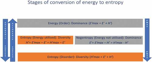
We have attempted to relate the well-studied indices of diversity and less studied dominance indices through energy-entropy relations (Figure 6). (Figure 6) showed the different stages for conversion of energy into entropy. When energy is utilised then entropy is equals to H’ = E’max – E’ = H’max – E’, and when system shows negentropy then energy equals to E’ = E’max – H’ = H’max – H’. When entropy shows order, in that case the maximum energy is equals to the sum of negentropy and entropy, and when entropy shows disordered, then maximium entropy is equal to the sum of negentropy and entropy.

Figure 6. Conversion of energy to entropy. E’_max: Maximum energy, H’_max: Maximum entropy, E’: Negentropy, H’: Entropy.

Palaghianu (2014) developed BIODIV software and compared diversity measures, and suggested that Shannon’s and Simpson’s indices are better measures for diversity evaluation and opined that Simpson’s indices for dominance and diversity evaluation have more flexibility for ecological interpretation. Justus (2011) also opined that various diversity indices employed for the study of communities, Shannon’s and Simpson’s indices are more popular. But based on certain criteria, the author proved that Simpson’s indices perform better than that of Shannon’s index. Brillouin’s index is also extensively used as an index of diversity. Therefore, we have taken Shannon’s, Simpson’s and Brillouin’s indices to develop dominance indices for our analysis at alpha, beta and gamma levels. Most of the β-diversity indices used in literature are based on the presence or absence of species in the samples. But we have used entropy-negentropy relations which are based on both the number of species and number of individuals per sample in our study. Koleff et al. (2003) listed 24 beta diversity indices using data on the presence or absence of species in quadrats, and recommended that the indices which exhibit homogeneity property under all circumstances perform better. Attempts to measure inter-habitat spatial diversity between two habitats separated by a distance (L), were made by Margalef (1958) with the equation (Sherwin & Prat, 2019),

$Heterogeneity=\frac{H_{pooled}-\left(H_1+H_2\right)/2}{L}$

where H is the Brillouin’s entropy. H is the average information per individual and is given as,

$H=\frac{1}{N}ln\left(\frac{N!}{N_1!N_2!\dots N_K!}\right)$

where, N is the total number of individuals of all the species, N_i is the number of individuals of different species, and K is the number of species. Buzas and Hayek (1996); Buzas & Hayek (2005) decomposed diversity (H) into two components, maximum and additive residual (E). The residual component is a measure of evenness and an inverse measure of richness.

$E=H_{max}-E_{obs.}$

It is seen from the study that negentropy can be used as a measure of dominance of a community. Entropy measures the uncertainty of a system, whereas negentropy measures its certainty (De Vries & Geva, 2009).

Jost (2007) stated that diversity is essentially partitioned into alpha, beta and gamma components. The three diversities are related either by additive law$\left(\gamma =\alpha +\beta \right)$, or by Whittaker’s multiplicative law$\left(\gamma =\alpha \beta \right)$. When the diversity indices are converted to number equivalents, or effective number of species, the multiplicative law is better. The best computational model for Simpson’s dominance and diversity is additive model (γ = α + β). Simpson’s β dominance and β diversity are calculated using the relation (γ – α), which can be applied to both single species and multispecies communities. The sum of Simpson’s β dominance and diversity is zero. The sum of Simpson’s dominance and diversity for α and beta diversities is 1. For communities having equal number of species, the sum of β_add (dominance) and β_add (diversity) is zero. Beck et al. (2013) hypothesised that rare species are less represented in small sample and underestimate their importance, thus affecting the robustness of the diversity evaluation. It is also seen that Harike wetland has higher diversity than Beas and Goindwal. Harike wetland has more favorable conditions than the other sides. Therefore, larger samples can produce better interpretation. It is therefore evident negentropy can be used as an index of dominance for a diversity index based on entropy of the community. We can extend the proposed negentropic dominance indices for community analysis at α, β and γ levels to provide better interpretation of the community structure.

Conclusions

We have proposed negentropic indices of dominance for Shannon’s entropy, Simpson’s information, Simpson’s inverse diversity and Brillouin’s entropy. Binary entropy functions give concave diversity curves, whereas binary negentropy functions give convex energy curves for dominance. Alpha negentropic index of dominance, α(E’), may be defined as the average dominance of M communities:

$\alpha \left(E^{\prime }\right)=\frac{1}{M}\sum _{j=1}^{M}E{ }_j^{\prime }$

where E’_j is negentropy of the j^th community.

Negentropic β index of dominance, β(E’) of a landscape, may be defined as,

$\beta \left(E^{\prime }\right)=\gamma \left(E^{\prime }\right)-\alpha \left(E^{\prime }\right)$

γ(E’), is gamma negentropic dominance index of the landscape consisting of M communities. Shannon’s and Simpson’s indices are more consistent at beta and gamma levels. The results of a case study on the Beas river indicate that on the basis of diversity indices Harike recorded maximum diversity followed by Beas and Goindwal Sahib. Based upon dominance, the Goindwal Sahib recorded maximum dominance of species, while Beas and Harike found low dominance. However, the combined results of dominance and diversity indices followed the trend as Harike > Beas > Goindwal Sahib for Shannon’s diversity and Simpson’s inverse diversity, nevertheless, for Simpson’s diversity the value remains constant. For Brillouin’s diversity index of dominance, the Harike recorded maximum diversity in contrast with Goindwal Sahib and Beas. Finally we can conclude that Harike wetland has higher diversity than Beas and Goindwal Sahib as revealed by results. It is therefore obvious negentropy may be applied as an index of dominance for a diversity index based on entropy of the community. We can extend the proposed negentropic dominance indices for community analysis at α, β and γ levels to provide better explanation of the community structure. The inferences obtained from the results of case study clearly revealed that diversity indices better explained the ecological information; however, in combination with dominance indices better results were obtained.¹

Acknowledgments

The authors are also thankful to the Department of Science and Technology, Government of India, New Delhi, for providing facilities under Special Assistance Programme.

Disclosure statement

No potential conflict of interest was reported by the author(s).

Notes

1. K: total number of species; α: average number of species; N: number of samples; g(S): species gained along gradient; l(S): species lost along gradient.

References

- Beck, J., Hollowway, J. D., Schwanghart, W., & Orme, D. (2013). Undersampling and the measurement of beta diversity. Methods in Ecology and Evolution, 4(4), 370–382. https://doi.org/10.1111/2041-210x.12023
- Berger, W. H., & Parker, F. L. (1970). Diversity of planktonic foraminifera in deep-sea sediments. Science, 168(3937), 1345–1347. https://doi.org/10.1126/science.168.3937.1345
- Brillouin, L. (1953). The negentropy principle of information. Journal of Applied Physics, 9(9), 1152–1163. https://doi.org/10.1063/1.1721463
- Brillouin, L. (1962). Science and Information Theory. Academic Press.
- Buzas, M. A., & Hayek, L. A. (1996). Biodiversity resolution: An integrated approach. Biodiversity Letters, 1(2), 40–43. https://doi.org/10.2307/2999767
- Buzas, M. A., & Hayek, L. C. (2005). On richness and evenness within and between communities. Paleobiology, 31(2), 199–220. https://doi.org/10.1666/0094-8373(2005)031 [0199:OR AEWA]2.0.CO ;2
- Cody, M. L. 1975. Towards a theory of continental speciesdiversities: bird distributions over Mediterranean habitatgradients. In: Cody, M. L. and Diamond, J. M. (eds), Ecology and evolution of communities. Harvard Univ. Press,pp. 214–257.
- Daly, A. J., Baetens, J. M., & De Baets, B. (2018). Ecological diversity: measuring the unmeasurable. Mathematics, 6(7), 119.
- De Vries, C. M., & Geva, S. (2009) Document Clustering with K-tree Christopher arXiv:1001.0827v1 [cs.IR]. h ttps://d oi.org/arXiv:10.100 7/978-3-6 42-03761 -0_43
- De Long Jr, D. C. (1996). Defining biodiversity. Wildlife Society Bulletin, 738–749.
- Dunne, J. A., & Williams, R. J. (2009). Cascading extinctions and community collapse in model food webs. Philosophical Transactions of the Royal Society B: Biological Sciences, 364(1524), 1711–1723.
- Guedes, E. B., De Assis, F. M., & Medeiros, R. A. (2016). Fundamentals of information theory. InQuantum zero-error information theory (pp. 27–63). Springer.
- Hammer, Ø., Harper, D. A., & Ryan, P. D. (2001). PAST: Paleontological statistics software package for education and data analysis. Palaeontol Electron, 4(1), 1–9. palaeo-electronica.org/2001_1/past/issue1_01.htm
- Harrison, S., Ross, S. J., & Lawton, J. H. (1992). Beta diversity on geographic gradients in Britain. The Journal of Animal Ecology, 1(1), 151–158. https://doi.org/10.2307/5518
- Jost, L. (2007). Partitioning diversity into independent alpha and beta components. Ecology, 88(10), 2427–2439. https://doi.org/10.1890/06-1736.1
- Justus, J. (2011). A case study in concept determination: Ecological diversity. In K. De Laplante, B. Brown, & K. A. Peacock (Eds.), Handbook of philosophy of science (Vol. 11, pp. 147–168). Elsevier.
- Koleff, P., Gaston, K. J., & Lennon, J. J. (2003). Measuring beta diversity for presence–absence data. Journal of Animal Ecology, 72(3), 367–382. https://doi.org/10.1046/j.1365-2656.2003.00710.x
- Kumar, V., Sharma, A., Bhardwaj, R., & Thukral, A. K. (2017, October 23–27) Phytosociology and Landsat TM data: A case study from river Beas bed, Punjab, India. In: 38th Asian Conference on Remote Sensing (ACRS.
- Kumar, V., Sharma, A., Bhardwaj, R., & Thukral, A. K. (2018). Comparison of different reflectance indices for vegetation analysis using Landsat-TM data. Remote Sensing Applications: Society and Environment, 12, 70–77. https://doi.org/10.1016/j.rsase.2018.10.013
- Margalef, R. (1958). Information theory in ecology. Journal of General Systems, 3, 36–71.
- Martin, J. S., Smith, N. A., & Francis, C. D. (2013). Removing the entropy from the definition of entropy: Clarifying the relationship between evolution, entropy, and the second law of thermodynamics. Evolution: Education and Outreach, 6(1), 1–9. https://doi.org/10.1186/1936-6434-6-30
- Morris, E. K., Caruso, T., Buscot, F., Fischer, M., Hancock, C., Maier, T. S., & Rillig, M. C. (2014). Choosing and using diversity indices: insights for ecological applications from the German Biodiversity Exploratories. Ecology and evolution, 4(18), 3514–3524.
- Mourelle, C., & Ezcurra, E. (1997). Differentiation diversity of Argentine cacti and its relationship to environmental factors. Journal of Vegetation Science, 8(4), 547–558.
- Palaghianu, C. (2014). A tool for computing diversity and consideration on differences between diversity indices. Journal of Land Management, 5(2), 78–82.
- Pandita, S., Kumar, V., & Dutt, H. C. (2019). Environmental variables vis-a-vis distribution of herbaceous tracheophytes on northern sub-slopes in Western Himalayan ecotone. Ecological Processes, 8(1), 45. https://doi.org/10.1186/s13717-019-0200-x
- Parkash, O., & Thukral, A. K. (2010). Statistical measures as measures of diversity. International Journal of Biomathematics, 3(2), 173–185. https://doi.org/10.1142/S179352451000091X
- Quarati, P., Lissia, M., & Scarfone, A. M. (2016). Negentropy in many-body quantum systems. Entropy, 18(2), 63. https://doi.org/10.3390/e18020063
- Renyi, A. (1961) On measures of entropy and information, in Proc. 4th Berkeley Symposium on Mathematical Statistics and Probability, Berkeley, pp. 547–561
- Sarangal, M., Buttar, G. S., & Thukral, A. K. (2012). Generating information measures via matrix over probability spaces. International Journal of Pure and Applied Mathematics : IJPAM, 81(5), 723–735.
- Schrödinger, E. (1944). What is life–the physical aspect of the living cell. Cambridge University Press.
- Semeniuk, V., & Cresswell, I. D. (2013). A proposed revision of diversity measures. Diversity, 5(3), 613–626.
- Shannon, C. E. (1948). A mathematical theory of communication. Bell System Technical Journal, 27(3), 379–423. https://doi.org/10.1002/j.1538-7305.1948.tb01338.x
- Sherwin, W. B., & Prat, I. F. N. (2019). The introduction of entropy and information methods to ecology by Ramon Margalef. Entropy, 21(8), 794. https://doi.org/10.3390/e21080794
- Simpson, E. H. (1949). Measurement of diversity. Nature, 163(4148), 688. https://doi.org/10.1038/163688a0
- Thukral, A. K. (2017). A review on measurement of alpha diversity in biology. Agricultural Research Journal, 54(10), 1–10. https://doi.org/10.1016/j.heliyon.2019.e02606
- Thukral, A. K., Bhardwaj, R., Kumar, V., & Sharma, A. (2019). New indices regarding the dominance and diversity of communities, derived from sample variance and standard deviation. Heliyon, 5(10), e02606. https://doi.org/10.1016/j.heliyon.2019.e02606
- Tilman, D., Isbell, F., & Cowles, J. M. (2014). Biodiversity and ecosystem functioning. Annual review of ecology, evolution, and systematics, 45, 471–493.
- Whittaker, R. H. (1960). Vegetation of the Siskiyou mountains, Oregon and California. Ecological Monographs, 30(3), 279–338. https://doi.org/10.2307/1943563
- Whittaker, R. H. (1972). Evolution and measurement of species diversity. Taxon, 21(2–3), 213–251. https://doi.org/10.2307/1218190
- Williams, P. H. (1996). Mapping variations in the strength and breadth of biogeographic transition zones using species turnover. Proceedings of the Royal Society of London. Series B: Biological Sciences, 263(1370), 579–588.
- Wilson, M. V., & Shmida, A. (1984). Measuring beta diversity with presence-absence data. The Journal of Ecology, 1055–1064.