Time-series analysis of landcover dynamics and their relation with coastline migration along Kuakata coast, Bangladesh using remote sensing techniques

ABSTRACT

Time-series analysis of satellite imageries is useful in studying changes in coastlines and the nature of the landcover dynamics in coastal environments. This study aimed to investigate the relationship between coastal erosion-accretion and landcover changes in Kuakata. Landsat TM and Landsat OLI/TIRS satellite imageries at a nearly 5-year interval between the years 1989 and 2020 were used to compare changes within five major landcover classes in the study area – 1) mangrove vegetation, 2) settlements, 3) agricultural land, 4) waterbody and 5) beach. Net land loss over the past 31 years was estimated to be 1.73 km² within the 93.05 km² study area. Linear regression rates were calculated to identify the area most prone to erosion. The average erosion rate along the coastline was estimated to be 2.09 m/year. Most erosion occurred along the western part of the coast while the highest accretion was limited to an area in the east. Study findings also suggested that changes in beach and mangrove vegetation classes have a significant spatial and statistical correlation with coastal erosion-accretion processes. These findings can help the policymakers implement coastal zonation, and preventive and rehabilitative measures to save the tourism industry and agriculture in Kuakata.

KEYWORDS:

• Kuakata
• landcover
• LULC
• DSAS
• coastal erosion
• coastline migration

Introduction

The erosion-accretion processes of the channels and islands of the Meghna estuarine delta make the coastline of Bangladesh highly dynamic. Most studies carried out on the changes in the coastline of Bangladesh indicate higher accretion than the erosion of the coasts ruled by estuarine conditions (Brammer, 2014; Islam et al., 2011). But this newly-formed land is less suitable for settlement and agriculture than older eroded land due to the raw state and alluvium salinity and is being continuously exposed to tidal and storm surge flooding. That’s why the land use and landcover of the coastal regions are unstable as well (Mondal et al., 2018). In a recent study on the positional change of the Ganges deltaic shoreline for the period of 1977–2017, it was found that the shoreline is shifting landward at an average linear regression rate of 0.27 m/year (Mullick et al., 2019). Examining the erosional processes can help the decision-makers, and administrators involved in coastal planning to understand the causes, develop forecasts, and plan how to implement preventive and rehabilitative measures (S. A. Hossain, Mondal, Thakur, Fadhil Al-Quraishi et al., 2022; S. A. Hossain, Mondal, Thakur, Linh et al., 2022).

Remote sensing techniques are extensively used to study changes in coastlines from time-series data (Mondal et al., 2021; White & El Asmar, 1999). Most studies suggest that the calculation of a single transform like the Normalized Difference Vegetation Index (NDVI) may be suitable for water delineation (M. A. Islam et al., 2014; Mondal et al., 2020). But the chaotic nature of the wave environment in the near-shore surf zone may result in high variability in the reflectance values in the red and infrared bands which is why they alone are unable to adequately separate the beach from the surf zone (Daniels, 2012). A hybrid algorithm for coastline delineation is likely to be preferable (Bushra, 2013; Daniels, 2012; Emran et al., 2017; Mullick et al., 2019). With the application of GIS, the accuracy of coastline delineation can be enhanced. Digitization is the most popular coastline delineation option (Rahman et al., 2013). Using high-tide coastlines is deemed to be the most convenient technique in case of unavailability of time and/or data on bathymetry and beach slope (A. Z. Z. Mondal et al., 2020; A. Z. Z. Islam et al., 2013). On the other hand, analyzing landcover changes from medium resolution images of coastal areas using supervised classifiers like SVM, ANN, fuzzy analysis and segmentation comprises complexity and bias (Yuan et al., 2009). This results in lower overall accuracy compared to unsupervised classification schemes in classifying homogeneous (50% pixels classified as one landcover class) study areas (Kaliraj et al., 2017; Peacock, 2014).

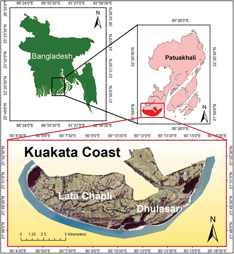
Kuakata, located at the southernmost tip of the coastline of Bangladesh is a panoramic beach that offers a full view of sunset and sunrise. In 2016, the total gross recreational benefit of this area was estimated to be approximately 29.55 million per year in Bangladeshi Taka (M. S. Hossain & Islam, 2016). Geographic demarcation of the area is 90° 4’ 12.0648” E, 21° 47’ 32.3628” N and 90° 16’ 52.6296” E, 21° 53’ 11.0256” N (Figure 1). This 93.05 km² coastal area at the north of the Bay of Bengal belongs to the Lata Chapli and Dhulasar unions of Kalapara Upazila in Patuakhali district within the Barishal division. Being part of the greater Ganges-Brahmaputra-Meghna (GBM) basin and Meghna Estuary, this area is susceptible to the estuarine processes of the river Galachipa and tidal actions of the Bay. It has a tropical climate with an average annual temperature of 26°C and about 2748 mm of precipitation occurs throughout the year (Climate-data.org, 2022). Its climate makes Kuakata prone to tropical cyclones (i.e., cyclone Sidr in 2007, cyclone Aila in 2009, cyclone Mahasen in 2013 etc.) and storm surges. Apart from that, coastal erosion and salinity intrusion are severe problems in the area, threatening tourism and agriculture there. The high and low-velocity longshore currents combined with the convex-shaped coastline makes Kuakata more susceptible to marine processes reflecting seasonal variations, and cause coastal erosion in some places and accretion in others (Bushra, 2013; Rashid & Mahmud, 2011). Previous studies on this coast suggest that more erosional activities occur along the coastline compared to coastal accretion (Bushra, 2013; A. Z. Z. A. Z. Z. Islam et al., 2013; Rahman et al., 2013). However, these studies on the Kuakata coast neither focused on landcover change analysis nor tried concluding the interrelationship between coastline shifting and subsequent landcover changes. But to mitigate the effects of coastal erosion and save the tourism in Kuakata, changes in landcover associated with erosion and accretion need to be explored. The present study aimed to determine whether any distinctive pattern exists relating coastal erosion and landcover dynamics of Kuakata.

Figure 1. Location map of the study area.

Materials and methods

Data set and pre-processing

For this study, satellite imageries (Landsat TM and Landsat OLI/TIRS) from 1989 to 2020 were used (Table 1). These images are from the same season of the respective years and were acquired around the same time of the day. All Landsat image bands have 30 m spatial resolution (bands used are listed in Appendix A).

Table 1. Overview of data used.

Dataset ID	Scene	Date of acquisition	Time of acquisition	Sensor
LT04_L1TP_137045_19890112_20170204_01_T1	P137R45	12 January 1989	03:57:39 UTC	TM
LT05_L1TP_137045_19940118_20170115_01_T1	P137R45	18 January 1994	03:46:32 UTC	TM
LT05_L1TP_137045_20010121_20161212_01_T1	P137R45	21 January 2001	04:05:06 UTC	TM
LT05_L1TP_137045_20061221_20161117_01_T1	P137R45	21 December 2006	04:19:55 UTC	TM
LT05_L1TP_137045_20101216_20161011_01_T1	P137R45	16 December 2010	04:15:04 UTC	TM
LC08_L1TP_137045_20150128_20170413_01_T1	P137R45	28 January 2015	04:25:10 UTC	OLI/ TIRS
LC08_L1TP_137045_20200110_20200114_01_T1	P137R45	10 January 2020	04:25:24 UTC	OLI/ TIRS

The Landsat images were downloaded in GeoTIFF format (USGS, 2019). These Landsat images had been radiometrically calibrated and orthorectified using ground control points (GCPs) and digital elevation model (DEM) data to correct for relief displacement (USGS, 2019).

Landcover classification

Experimentation was done using both supervised and unsupervised pixel-based classification algorithms but an unsupervised clustering algorithm was chosen for this research over a supervised algorithm. Because these clustering algorithms seek to find classes that are most different while supervised algorithms based on training data were causing a higher level of lumping between classes. Among various clustering algorithms, ISODATA was used in this study. The images were initially classified into 100 landcover classes from which they were recoded to 7 broad classes – 1) mangrove vegetation, 2) settlements, 3) dry agricultural land, 4) wet agricultural land, 5) inland waterbody, 6) sea, and 7) beach based on ground data and visual interpretation. Dry and wet agricultural lands were later merged as “agricultural land” while inland and sea water were merged to become a single class called “waterbody” to reduce complexity in change detection.

Validation of landcover classifications and post-classification comparison

A four-day field campaign was carried out in the study area focusing especially along the coastline to collect ground data on high waterlines and landcover types, as well as GPS coordinates using a handheld device. One hundred and forty-two ground data points were collected which were then used for calculating four accuracy metrics to evaluate classification accuracy – overall accuracy, kappa coefficient, user’s accuracy, and producer’s accuracy.

Change detection was performed between successive pairs of classified Landsat images to show the sequence of change and also between the first date and last date to show the resultant changes over the study years.

Coastline extraction and erosion rate calculation

For coastline delineation, a hybrid algorithm using NDVI (Normalized Difference Vegetation Index) and Tasseled Cap Analysis followed by ESRI’s unsupervised ISO classification was used in this study (Daniels, 2012; Mondal et al., 2020). In the case of NDVI, vegetative “spectral signatures” are calculated based on the principle that “actively growing green plants strongly absorb radiation in the visible region of the spectrum and strongly reflect radiation in the NIR region” (Sultana et al., 2014).

Tasseled Cap Analysis is based on a linear transformation of data from the original image into three new axes (brightness, greenness, and wetness) which become features of the transformation and allows the creation of other useful raster by-product files like polylines (coastlines; Scott et al., 2003; Vorovencii, 2007). These three bands and the NDVI band were used for ESRI’s unsupervised ISO classification algorithm to obtain a binary classification of land and sea for all seven Landsat images (Daniels, 2012). Then the coastlines were extracted using GIS functions – majority filtering, contour, smooth line, and finally, manual editing to correct for overlapping of other features. Additionally, the 7-class unsupervised ISODATA classified Landsat images were reclassified to land and sea to extract erosional and accretional polygons of each study year. These polygons were used for calculating total coastal erosion and accretion in 5-year windows (1989–1994, 1994–2001, 2001–2006, 2006–2010, 2010–2015, 2015–2020, and 1989–2020), as well as between the study years of 1989–2020.

Erosion rates for the extracted coastlines were calculated automatically in Digital Shoreline Analysis System (DSAS) version 5.0 at 30-m interval transects (Himmelstoss et al., 2018). As collecting data for the total uncertainty term is time-consuming and expensive, it was ignored. Instead, the coastlines were collected from the same season to reduce the magnitude of uncertainty (Ruggiero & List, 2009).

Results

Landcover classification, results validation and post-classification comparison

The total area of each landcover class for the years 1989, 1994, 2001, 2006, 2010, 2015, and 2020 in km² (Figure 3) was estimated from the unsupervised ISODATA classification of Landsat images (Figure 2). It is seen that even though the share of agricultural lands had been reducing over the years, it is still the most dominant landcover class in the study area. Despite the afforestation attempts of forest division, mangrove vegetation has been reduced to some extent. However, the area coverage of this class has increased in 2020 compared to 2015. The most increase in area is seen in the settlements class.

Figure 2. Landcover classification results of Landsat images from 1989 to 2020.

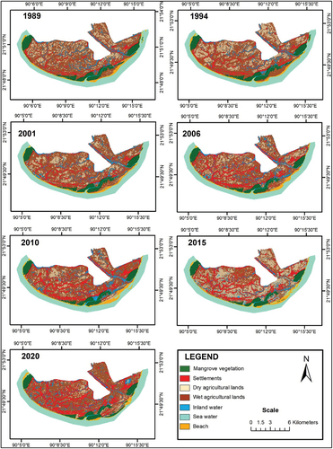
Figure 3. Total area (km²) occupied by landcover types from the year 1989 to 2020.

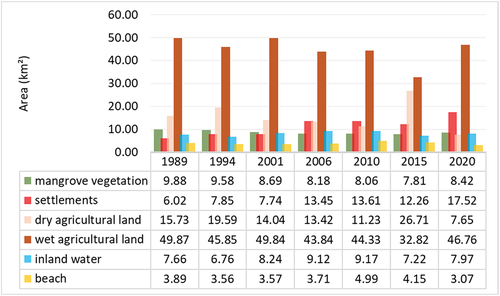
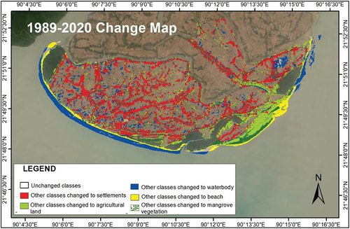
The total beach area has been fluctuating over the years due to erosional and accretional activities. The highest accretion occurred between 1994 and 2010 after which the beach area started decreasing, and reaching the lowest value of this class in 2020. It indicates that the overall erosion rates were highest from 2010 to 2020. The drastic changes in landcover classes between 1989 and 2020 are shown in Figure 4.

Figure 4. Generalized landcover class changes from 1989 to 2020.

Validation of image classification was done by calculating accuracy metrics (Table 2) from the confusion matrix (Appendix C) generated using the ground truth data against the pixel data from the Landsat OLI image of 2020.

Table 2. Image classification accuracy assessment results.

Landcover class	User’s Accuracy	Producer’s Accuracy	Overall Accuracy	Kappa Coefficient
Mangrove vegetation	100%	73%	83.1% (approximately)	0.79 (approximately)
Settlements	91%	68%
Agricultural land	63%	100%
Waterbody	72%	100%
Beach	100%	87%

Change detection results (Appendix B) suggest that mangrove vegetation was mostly changed to water class (Figure 4). We can assume this occurs due to wave actions causing coastal erosion. Over the years, 1.51 km² of mangrove forests were consumed by the sea. From 1989 to 2020, 0.72 km² of mangrove vegetation was changed to agricultural land, and the 0.59 km² changed to beach were most likely to occur due to the erosion of mangrove areas and subsequent coastal accretion. In the case of settlements, it is seen that between 1989 and 2020 about 1.22 km² were converted to agricultural land. It indicates that the settlement vegetation was cleared for agricultural purposes. But the highest change of 3.04 km² occurred between 2010 and 2015. 0.67 km² of settlements were changed to inland water while 0.15 km² of settlements were changed to beach features during the study years. This can be explained as the combined result of coastal erosion-accretion processes and forestation attempts. The same can be said for the changes in agricultural lands to beach and mangrove class. In fact, the most dramatic change has been observed in agricultural use. From 1989 to 2020, 11.68 km² of agricultural land was changed to settlements, and 4.95 km² were lost to waterbodies (Figure 5). 1.84 km² of beach area were lost to the sea and 1.21 km² were changed for agricultural purposes during the study years (Figure 6).

Figure 5. Major interclass changes from 1989 to 2020.

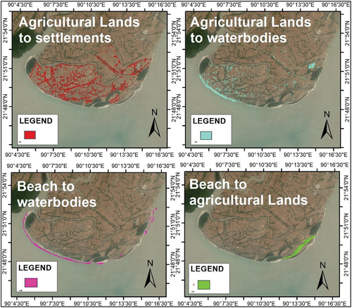
Figure 6. Major interclass changes from 2015 to 2020.

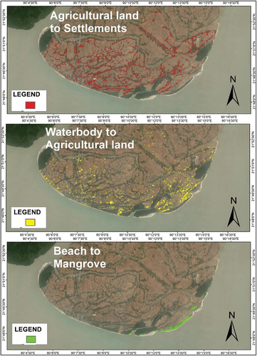
Change detection results also suggest that mostly waterbodies were changed to agricultural lands, the highest being 3.50 km² between 2015 and 2020 (Figure 6). This indicates sediment deposition was highest during this period that allowed the newly formed land to be used for agriculture.

Coastline extraction and erosion rate calculation

In this study, linear regression rates (LRR) were chosen to present the computational results of DSAS. LRR is determined by fitting a least-squares regression line to all coastline points for a transect so that the sum of the squared residuals is minimized. LRR is the slope of the line whose positive and negative values correspond to coastal accretion and erosion (Figure 7(b) and Table 3), respectively (Sutikno, 2016).

Figure 7. (a) Zones of erosion and accretion between 1989–2020; (b) LRR along the coastline.

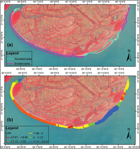
Table 3. Summary statistics of erosion rate calculation.

percent of all transects that are erosional	71.78%	percent of all transects that are accretional	28.22%
maximum value erosion (meters/year)	−47.67	maximum value accretion (meters/year)	23.51
average of all erosional rates (meters/year)	−8.03	average of all accretional rates (meters/year)	13.04

It can be seen that erosion rates are highest along the western coast facing the bay while accretion rates are higher at estuary mouths on both sides of the coastline.

Total eroded and accreted areas extracted from unsupervised ISODATA classification of 1989 and 2020 images (Figure 7a) seem to correspond to the LRR calculated by DSAS. Areas having negative LRR are found to be eroded while areas having positive LRR are attributed to accretional areas. Based on these results, it can be said that most erosion occurred along the western part of the coast while accretion was highest in a limited area in the eastern part. From 1989 to 2020, 4.76 km² of coastal land was eroded while 3.03 km² was accreted in Kuakata. So, the net land loss over the past 31 years is 1.73 km² (Figure 8).

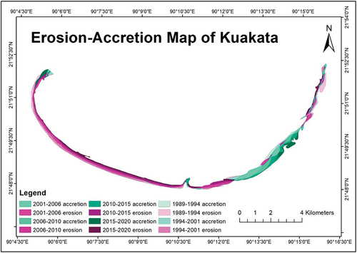
Figure 8. Eroded and accreted areas in Kuakata at 5-year intervals from 1989 to 2020.

Relationship between coastal erosion and landcover dynamics

The graphical representation of the relationship between changes in major landcover classes and coastline movement in the study area is shown in Figure 9.

Figure 9. Landcover changes shown as percentages vs. coastline movement in km². Negative values indicate the percentage by which the share of each landcover class has been decreased during the 5-year interval while positive values indicate an increase. The total area of coastal erosion and accretion during the time interval are shown on the secondary axis.

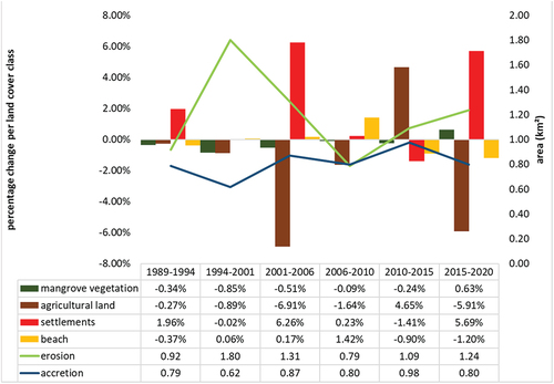
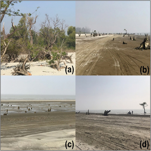
It can be realized that erosion and accretion are a continuous process along the coastline. In the case of accretion, the trend was alternating increase and decrease every 5 years. However, the trend in erosion was not similar. From 1994 to 2010, the total eroded area per 5 years was on the decline and the lowest value being 0.79 km² between 2006 and 2010. In fact, 2006–2010 was the only period when the total eroded area was a little lower than the total accreted area. It means during this period some overall gain may have occurred along the coast. But after 2010, the total eroded area had been increasing per 5 years that means continuous erosion had been occurring along the coast in the past decade. In the case of landcover changes, mangrove vegetation was shown to be on the decline until 2015. Such a scenario was also evidenced by field observation (Figure 10).

Figure 10. (a) and (b) denuded forests on the coast of Dhulasar; (c) denuded mangrove vegetation on the western coast of Lata Chapli; (d) seawater encroachment into forests near Dhulasar coast.

Agricultural land share showed a decreasing trend, the exception being during 2010–2015 when a significant increase was noticed (Figure 9). That is also the period when the highest coastal accretion occurred. On the other hand, the settlements class shows an increasing trend in area coverage that is only natural due to population rise. But an exception was noticed between 2010 and 2015 when it showed a decrease. The loss due to erosion will not be reflected in the statistics of this class as the change will be shared by other classes. To truly understand the change, we have to take a look at Figure 11 which shows the settlement areas that were lost to coastal erosion.

Figure 11. Landcover changes specific to the accretional and erosional zones between 1989 to 2020.

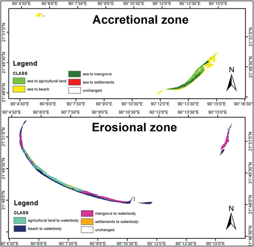
It can be seen that major classes – mangrove forests, beaches and agricultural lands were lost to erosion and these classes are now changed to seawater. On the western part of the coast, roads, embankments, and beachside settlements were lost due to erosion. Beach class, however, shows a very high correlation with coastal erosion (Figure 9). From 1994 to 2010, erosion per 5 years was on the decline while the percent change of beach area was on the rise. Again during 2010–2020, the beach area had been declining while the total eroded area has increased per 5-year interval.

Discussion

This study aims to explore the relationship between coastal erosion and landcover changes in Kuakata. It was evident that as long as erosion continues, so will the mangrove deforestation. If afforestation efforts succeed then there may be an overall gain in mangrove forest share which is the case occurring between 2015 and 2020 (Figure 9). According to the Gongamati Reserved Forest Range officer, afforestation efforts on accretional lands of the Dhulasar coast started in 2007. The second phase of the plantation project was carried out in 2011. These efforts resulted in an increase of 0.85 km² in mangrove vegetation between the study years.

The 1.72 km² of waterbodies changed to settlements (Appendix B) attributes to river sedimentation allowing settlement build-up. The decrease in settlement area between 2010 and 2015 (Figure 9) could be due to the impact of Cyclone Mahasen in 2013 which had devastating impacts on infrastructures and settlements in the Patuakhali district. As the population grows, the settlement area is bound to expand. When one region is flooded or eroded, families relocate landwards and compensate for the loss of housing and infrastructure by clearing forests or using up agricultural lands for settlement purposes.

1.28 km² of the beach area was accreted between 1989 and 2020 (Appendix B). But accretion rates are much lower than erosion rates as sediment deposition and settlement is a slow process. Even though there is no net land gain in the study area, coastal accretion does occur. Initially, the newly accreted lands are shown to be beach feature class. Later on, they are either changed to mangrove vegetation or agricultural land.

Similar study can be conducted on the entire coast of Bangladesh since previous studies on the coastline of Bangladesh focused only on the erosion rates, not the implications in landcover changes. In addition, considering total uncertainty terms should provide more accurate erosion rates.

Conclusion

Kuakata beach, an important tourist destination in Bangladesh is subjected to continuous coastal erosion-accretion processes over the years and currently, this scenic landscape is on the brink of disappearance. Interaction between two strong opposing factors – fluvial delta-building activities and marine processes results in this dynamism. Along the coast, accretion and erosion are taking place at different rates and the natural environments are being changed in various ways by human interventions. The findings from this study suggest that beach and mangrove vegetation are most affected by coastal erosion-accretion processes and changes in these classes have a significant correlation with coastal processes. In order to save the tourism of this economically and aesthetically significant area, appropriate beach protection measures should be taken in the areas shown to be most prone to coastal erosion. Newly accreted areas can be considered for relocation of the tourism industry and future developments in Kuakata.

Acknowledgments

This research work was carried out at the Department of Disaster Science and Management, University of Dhaka and the authors are grateful for such a research opportunity. Landsat imageries used in this study are courtesy of the U.S. Geological Survey. The authors convey their thankfulness to Gongamati Forest Division for their co-operation during field observation.

Disclosure statement

No potential conflict of interest was reported by the author(s).

Appendix A

Table A1. Image bands used for the study.

Landsat TM		Landsat OLI/TIRS
Bands	Wavelength (micrometers)	Bands	Wavelength (micrometers)
Band 1 – Blue	0.45–0.52	Band 1 – Ultra Blue (coastal/ aerosol)	0.435–0.451
Band 2 – Green	0.52–0.60	Band 2 – Blue	0.452–0.512
Band 3 – Red	0.63–0.69	Band 3 – Green	0.533–0.590
Band 4 – NIR	0.76–0.90	Band 4 – Red	0.636–0.673
Band 5 – Shortwave Infrared (SWIR) 1	1.55–1.75	Band 5 – NIR	0.851–0.879
Band 7 – SWIR 2	2.08–2.35	Band 6 – SWIR 1	1.566–1.651
		Band 7 – SWIR 2	2.107–2.294
		Band 9 – Cirrus	1.363–1.384

Appendix B

Table B1. Landcover change (km²) matrix.

Change Results	1989–1994	1994–2001	2001–2006	2006–2010	2010–2015	2015–2020	1989–2020
Mangrove vegetation changed to other classes
Settlements	0.1233	0.0648	0.1251	0.0567	0.1908	0.1188	0.0972
Agricultural land	0.2709	0.3402	0.2412	0.0918	0.2898	0.1233	0.7236
Waterbody	0.198	0.4014	0.3933	0.2358	0.1575	0.1278	1.5147
Beach	0.4815	0.4293	0.1962	0.3348	0.1143	0.1728	0.5868
Settlements changed to other classes
Mangrove	0.1701	0.1098	0.0378	0.1953	0.0567	0.0279	0.0639
Agricultural land	1.2843	1.422	0.3816	2.2275	3.0384	1.2141	1.2195
Waterbody	0.2583	0.9117	0.5031	0.3996	0.6579	0.4348	0.666
Beach	0.0018	0.0486	0.0738	0.0486	0	0.0108	0.1539
Agricultural land changed to other classes
Mangrove	0.2493	0.1125	0.2376	0.1584	0.0972	0.3294	0.4194
Settlements	2.7063	1.9278	5.4288	1.7334	1.8639	6.2406	11.6757
Waterbody	1.7631	2.5155	2.6955	3.5847	3.2445	3.9348	4.9545
Beach	0.2628	0.6903	0.5067	1.0332	0.1908	0.2196	0.4545
Beach changed to other classes
Mangrove	0.0666	0.0198	0.0936	0.018	0.1926	0.6507	0.1305
Settlements	0.0189	0.0018	0.0018	0	0.0054	0.0009	0.1143
Agricultural land	1.107	0.2997	0.2592	0.0846	0.5346	0.7641	1.2096
Waterbody	0.7587	1.476	1.278	0.9729	1.6191	1.1241	1.8405
Waterbody changed to other classes
Mangrove	0.2799	0.1053	0.0756	0.2322	0.1539	0.1485	0.8478
Settlements	0.6966	0.3906	1.1475	1.2411	0.3591	0.5841	1.7217
Agricultural land	2.1492	1.6335	1.3607	2.4075	2.0097	3.5001	3.1599
Beach	0.8694	0.6471	0.9918	0.9432	0.0684	1.0575	1.2789

Appendix C

Table C1. Landsat OLI 2020 confusion matrix.

Class		Reference Data					Ground Truth Totals
		Mangrove vegetation	Settlements	Agricultural land	Water body	Beach
Classified Data	Mangrove vegetation	27	0	0	0	0	27
	Settlements	1	21	0	0	1	23
	Agricultural land	3	10	26	0	2	41
	Waterbody	6	0	0	18	1	25
	Beach	0	0	0	0	26	26
Total		37	31	26	18	30	142

References

- Brammer, H. (2014). Bangladesh’s dynamic coastal regions and sea-level rise. Climate Risk Management, 1, 51–62. https://doi.org/10.1016/j.crm.2013.10.001
- Bushra, N. (2013). Detecting Changes of Shoreline at Kuakata Coast Using RS-GIS Techniques and Participatory Approach [Bangladesh University of Engineering and Technology]. http://lib.buet.ac.bd:8080/xmlui/bitstream/handle/123456789/4186/FullThesis.pdf?sequence=1&isAllowed=y
- Climate-data.org. (2022). Kuakata climate. https://en.climate-data.org/asia/bangladesh/barisal-division/kuakata-969757/
- Daniels, R. C. (2012). Using arcmap to extract shorelines from landsat TM & ETM+ Data. Thirty-Second ESRI International Users Conference Proceedings, San Diego, CA, 6. ESRI. https://proceedings.esri.com/library/userconf/proc12/papers/432_61.pdf
- Emran, A., Rob, M. A., & Kabir, M. H. (2017). Coastline change and erosion-accretion evolution of the Sandwip Island, Bangladesh. International Journal of Applied Geospatial Research, 8(2), 33–44. https://doi.org/10.4018/IJAGR.2017040103
- Himmelstoss, E. A., Henderson, R. E., Kratzmann, M. G., & Farris, A. S. (2018). Digital Shoreline Analysis System (version 5.0): U.S. Geological Survey software release. Reston, Virginia: U.S. Department of the Interior, U.S. Geological Survey. https://code.usgs.gov/cch/dsas
- Hossain, M. S., & Islam, A. K. M. N. (2016). Estimating recreational benefits of the kuakata sea beach: a travel cost analysis. Daffodil International University Journal of Business and Economics, 10(2), 26–40. https://www.researchgate.net/publication/318085014_Estimating_Recreational_Benefits_of_the_Kuakata_Sea_Beach_A_Travel_Cost_Analysis
- Hossain, S. A., Mondal, I., Thakur, S., Linh, N. T. T., & Anh, D. T. (2022). Assessing the multi-decadal shoreline dynamics along the Purba Medinipur-Balasore coastal stretch, India by integrating remote sensing and statistical methods. Acta Geophysica, 2022, 1–15. https://doi.org/10.1007/S11600-022-00797-5
- Hossain, S. A., Mondal, I., Thakur, S., & Fadhil Al-Quraishi, A. M. (2022). Coastal vulnerability assessment of India’s Purba Medinipur-Balasore coastal stretch: A comparative study using empirical models. International Journal of Disaster Risk Reduction, 77, 103065. https://doi.org/10.1016/j.ijdrr.2022.103065
- Islam, M. A., Majlis, A. B. K., & Rashid, M. B. (2011). Changing Face of Bangladesh Coast. The Journal of NOAMI, 28(1).
- Islam, A. Z. Z., Kabir, S. M. H., Nur, M., & Sharifee, H. (2013). High-tide coastline method to study the stability of kuakata coast of bangladesh using remote sensing techniques. Asian Journal of Geoinformatics, 13(1), 23–29. http://203.159.29.7/index.php/journal/article/viewFile/119/59
- Islam, M. A., Hossain, M. S., Hasan, T., & Murshed, S. (2014). Shoreline changes along the Kutubdia Island, South East Bangladesh using digital shoreline analysis system. The Bangladesh Journal of Scientific Research, 27(1), 99–108. https://doi.org/10.3329/bjsr.v27i1.26228
- Kaliraj, S., Chandrasekar, N., Ramachandran, K. K., Srinivas, Y., & Saravanan, S. (2017). Coastal landuse and land cover change and transformations of Kanyakumari coast, India using remote sensing and GIS. Egyptian Journal of Remote Sensing and Space Science, 20(2), 169–185. https://doi.org/10.1016/j.ejrs.2017.04.003
- Mondal, I., Thakur, S., Ghosh, P., De, T. K., & Bandyopadhyay, J. (2018). Land use/land cover modeling of Sagar Island, India using remote sensing and GIS techniques. Advances in Intelligent Systems and Computing, 755, 771–785. https://doi.org/10.1007/978-981-13-1951-8_69
- Mondal, I., Thakur, S., Juliev, M., Bandyopadhyay, J., & De, T. K. (2020). Spatio-temporal modelling of shoreline migration in Sagar Island, West Bengal, India. Journal of Coastal Conservation, 24(4), 1–20. https://doi.org/10.1007/s11852-020-00768-2
- Mondal,I., Thakur,S., Ghosh,P., & De,T.K.(2021).Assessing the Impacts of Global Sea Level Rise (SLR) on the Mangrove Forests of Indian Sundarbans Using Geospatial Technology.InS. Singh,S. Kanga, G.Meraj, & M. Farooq(Eds.), Geographic Information Science for Land Resource Management(pp.209–227).Wiley.https://doi.org/10.1002/9781119786375.CH11
- Mullick, M. R. A., Islam, K. M. A., & Tanim, A. H. (2019). Shoreline change assessment using geospatial tools: A study on the Ganges deltaic coast of Bangladesh. Earth Science Informatics, 13(2), 299–316. https://doi.org/10.1007/s12145-019-00423-x
- Peacock, R. (2014). Accuracy Assessment of Supervised and Unsupervised Classification Using Landsat Imagery of Little Rock, Arkansas. [Northwest Missouri State University]. http://www.nwmissouri.edu/library/theses/2014/PeacockRexA.pdf
- Rahman, A., Mitra, M. C., & Akter, A. (2013). Investigation on erosion of Kuakata sea beach and its protection design by artificial beach nourishment. Journal of Civil Engineering (IEB), 41(1), 1–12. https://www.researchgate.net/publication/308776753_Investigation_on_erosion_of_Kuakata_sea_beach_and_its_protection_design_by_artificial_beach_nourishment
- Rashid, M. B., & Mahmud, A. (2011). Longshore current and its effect on Kuakata beach, Bangladesh. Bangladesh Journal of Geology, 29–30, 30–40. https://www.researchgate.net/publication/323550576_Longshore_Current_and_Its_effect_on_Kuakata_Beach_Bangladesh
- Ruggiero, P., & List, J. H. (2009, September). Improving accuracy and statistical reliability of shoreline position and change rate estimates. Journal of Coastal Research, 255, 1069–1081. https://doi.org/10.2112/08-1051.1
- Scott, J. W., Moore, L. R., Harris, W. M., & Reed, M. D. (2003). Using the landsat 7 enhanced thematic mapper tasseled cap transformation to extract shoreline. Report No. 2003-272. U.S. Geological Survey. https://doi.org/10.3133/ofr2003272
- Sultana, S. R., Ali, A., Ahmad, A., Mubeen, M., Zia-Ul-Haq, M., Ahmad, S., Ercisli, S., & Jaafar, H. Z. E. (2014). Normalized difference vegetation index as a tool for wheat yield estimation: A case study from Faisalabad, Pakistan. The Scientific World Journal, 2014, 1–8. https://doi.org/10.1155/2014/725326
- Sutikno, S. (2016). Integrated remote sensing and GIS for calculating shoreline change in rokan estuary. KnE Engineering, 1(1). https://doi.org/10.18502/keg.v1i1.491
- USGS. (2019). Landsat Collection 1. https://www.usgs.gov/land-resources/nli/landsat/landsat-collection-1?qt-science_support_page_related_con=1#qt-science_support_page_related_con
- Vorovencii, I. (2007). Use of the “ Tasseled Cap ” transformation for the interpretation of satellite images. RevCAD Journal of Geodesy and Cadastre, 2007(07), 75–82. https://www.researchgate.net/publication/259479299_Use_of_the_Tasseled_Cap_Transformation_for_the_Interpretation_of_Satellite_Images
- White, K., & El Asmar, H. M. (1999). Monitoring changing position of coastlines using thematic mapper imagery, an example from the nile delta. Geomorphology, 29(1–2), 93–105. https://doi.org/10.1016/S0169-555X(99)00008-2
- Yuan, H., Van Der Wiele, C., & Khorram, S. (2009). An automated artificial neural network system for land use/land cover classification from landsat TM imagery. Remote Sensing, 1(3), 243–265. https://doi.org/10.3390/rs1030243