Groundwater potential zones identification and validation in Peninsular India

ABSTRACT

Groundwater mapping is essential for meeting the water requirement of people. Identification of groundwater potential zone was attempted for a watershed located in Kanchipuram district, Tamil Nadu, India. The Landsat 8 and Landsat 5 data were used for land use/land cover analysis. For delineating groundwater potential zone, total seven thematic layers namely drainage density, slope, geology, soil, geomorphology, rainfall, land use/land cover and observed groundwater levels were considered during the analysis. Afterwards thematic layers were converted into raster using GIS platform. Further, after assigning weights and ratings to each thematic layer, overlay analysis was applied and total five zones were delineated as very good, good, moderate, poor, and very poor. The majority of area has moderate groundwater potential zone. The potential zone map was also validated using ROC method. The map of 2005 shows a highest accuracy compared to rest year maps.

KEYWORDS:

• Overlay analysis
• thematic layer
• receptor operating curve
• groundwater
• peninsular India

Introduction

Groundwater is an important natural resource used in different sectors, namely, domestic, agriculture and industrial (Singh et al., 2009). In India, majority of population depends on groundwater (Singh et al., 2010) and also in the world because groundwater act as alternative source to surface water (Arabameri et al., 2019). Therefore, mapping and monitoring of groundwater resources are very important in semi-arid and arid areas (Subba Rao & Prathap Reddy, 2004; Subba Rao et al., 2013).

Literature outlined the role of remote-sensing and geographical information system (GIS)-based multi-criteria decision-making (MCDM) analysis (Singh et al., 2018; Kumar et al., 2022), analytic hierarchy method (Agarwal et al., 2013), fuzzy logic technique (Mohamed & Elmahdy, 2017), influencing factors analysis (Chowdhury et al., 2010; Das & Mukhopadhyay, 2020; Magesh et al., 2012), and Dempster-Shafer model (Pandey et al., 2022) for delineation of groundwater potential zones (GWPZs). The remote-sensing and GIS have many advantage over the conventional methods (Tweed et al., 2014; Zolekar & Bhagat, 2015) such as time and cost-effective and provide synoptic coverage.

Studies reported that for delineation GWPZ mainly required input data such as on land use/land cover (LULC), relief, slope, drainage density, lithology, geological structures, soil, geomorphology, water level, rainfall, and others (Murmu et al., 2019; Pande et al., 2021; Singh et al., 2010). The GWPZs can be assisted by surveys, namely, geophysical, hydrogeological, geological, drilling and satellite data, global positioning system data and GIS (Subba Rao, 2006, 2016; Kumar et al., 2008; Mondal et al., 2008; Subba Rao et al., 2016). However, direct methods are time-consuming, cost-intensive and required a skilled manpower (Fetter, 1994). The combination of earth observation satellite data and GIS gives an information about the different effective components of groundwater existence and its movement corresponding to the geology, soils, geomorphology, LULC, drainage density, geology, and lineaments (Jha et al., 2007; Subba Rao, 2011 Yadav et al., 2018 Kumar et al., 2018 Kumar et al., 2020). These factors can play an important role in identification and evaluation of GWPZs (Thomas et al., 1999). Overlay analysis of thematic layers in GIS environment help to identify the occurrence of groundwater (Kumar et al., 2008; Nagarajan & Singh, 2009). Therefore, our objective of present study was to delineate the GWPZs using integrated method and to validate the output using Receptor Operating Curve (ROC) method for a watershed located in Kanchipuram, Tamil Nadu, India.

Study area

The district Kanchipuram is located in the southern part of India (Figure 1). The Kanchipuram has a total geographical area of 1909.58 km². The land is flat and aspect is towards the south and east with average elevation is 83.2 m above mean sea level, whereas in east it is bound by Bay of Bengal. Agriculture is dominant class and 47% of population engaged in agriculture activities (Rawat et al., 2019). The climate is humid and hot and region receives the rain under the north-east and south-west monsoons. Relative humidity in November to January varies from 83 to 84%; however, in June, it is around 58%. The minimum and maximum temperature is 20°C and 37°C, respectively.

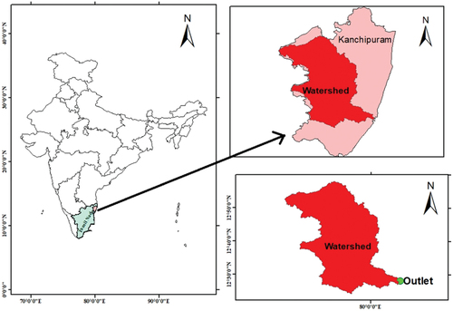
Figure 1. The map show a location of study area.

Physiography

The major portion is on undulating topography with countless depressions and has many natural tanks which are used for irrigation purpose. Based on Geological Survey of India, the region has three major geomorphic units namely erosional (Chingleput-Tirukkalukkunram surface), fluvial (Palar surface), and marina (Mahabalipuram surface). The drainage pattern is radial and drainage network is sub-dendritic.

Data sets and sources

Total seven types of dataset were collected and processed. Landsat 8 (4 February 2020, 14-Octo-2015), and Landsat 5 (16-Octo-2010, 11 May 2005) data sets have downloaded from web portal: https://earthexplorer.usgs.gov/ and pre-processed before further analysis. Rainfall data in grid format were downloaded from (https://crudata.uea.ac.uk/cru/data/hrg/) CRU TS 2.1 Global Climate Database (The CRU TS2.1 Climatic Research Unit (CRU) of University of East Anglia has produced climate dataset). The SRTM 30 m digital elevation model data were downloaded from web portal: https://earthexplorer.usgs.gov/ and used for slope and relief analysis. Geology and geomorphology of study area was collected from Bukhosh portal of Geological Survey of India (https://bhukosh.gsi.gov.in/Bhukosh/Public), and soil map was downloaded from Food and Agricultural Organization (FAO) web portal: https://www.fao.org/soils-portal/data-hub/soil-maps-and-databases/en/. The observed groundwater level data for validation were downloaded from Central Ground Water Board (CGWB), India web portal: http://cgwb.gov.in/GW-data-access.html. Global Positioning System (GPS, eTrex Legend® HCx, with ± 15 m accuracy) was selected for collection of co-ordinates of all training samples for supervised classification of satellite data.

Methodology

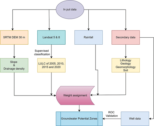
Land use/land cover (LULC) of different years was prepared using Landsat 5 and 8 satellite data. Geomorphology, and geology maps were prepared from resource atlas and soil map from Food and Agriculture Organization (FAO) soils portal (www.fao.org/soils-portal/data-hub/soil-maps-and-databases/). The drainage network and slope map were prepared from SRTM 30 m DEM and with the help of drainage map, and drainage density map was generated in GIS platform using density analysis tool. The total annual rainfall distribution map of different years were prepared using inverse distance weighted interpolation of point rainfall data in GIS platform. Rank and weights were assigned to each layer. Further, these layers were integrated using weighted overlay analysis (WOA). The weight for the selected thematic layer was calculated based on Saaty’s scale (1980). The particular layer and their class has assigned a weightage and a rank ranging from 1 (low GWPZ) to 5 (high GWPZ), respectively.

The GWPZ map was prepared and categorized into five classes namely very good, good, moderate poor and very poor. The Cumulative Score Index (CSI) method was used for this classification. The CSI expression is as follows (eqn. 1):

CSI = Σ (Drainage density rank x weight + Geology rank x weight + Geomorphology rank x weight +LULC rank x weight + Rainfall rank x weight + Soil rank x weight + Slope rank x weight)

(1) $\mathrm{CSI}={\int }_{\mathrm{i}=1}^{\mathrm{n}}{\int }_{\mathrm{j}=1}^{\mathrm{m}}{\mathrm{W}}_{\mathrm{j}}\times {\mathrm{X}}_{\mathrm{i}}$(1)

where W_j is the normalized weight of the j^th factor; X_i is the rank of the i^th classes/features of athematic layer; m (8) is the total number of thematic layers; and n is the total number of classes/features (5) in a thematic layer (Suja Rose & Krishnan, 2009). The schematic flow chart of the methodology is showed in Figure 2.

Figure 2. The schematic diagram show the adopted methodologies in the study.

Result and discussion

The detail of different factors mentioned in following section given below:

Drainage density (D_d)

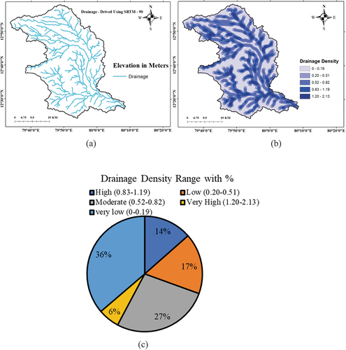
Majority of drainage is found in upper and middle portion and low flow of water at upper to lower part of watershed due to low slope. In rainy season, all drainages have maximum of water and almost flood condition because the watershed is located in low lying area. In case of GWPZ, natural drainage systems (Figure 3(a)) have importance to govern the water directly on the surface because more number of drainage is a sign of more possibility of water to drain out (Yadav et al., 2020 Yadav et al., 2020; Kumar and Singh, 2021 Singh and Singh, 2022). While poor drainage network in any region will have low possibility of good GWPZ. The study area comes under the 6^th order drainage system. The D_d map was developed (Figure 3(b)) using following formula (eq. 2) proposed by Horton (1932);

Figure 3. (a) A drainage network map of study area, and (b) A drainage density map of study area (c) The drainage density distribution graph of study area.

(2) $\mathrm{Drainage}\mathrm{Density}\left({\mathbf{D}}_{\mathbf{d}}\right)\mathit{\hspace{0.17em}}={\sum }_{\mathbf{i}=0}^{\mathbf{n}}\frac{{\mathbf{D}}_{\mathbf{i}}}{\mathbf{A}\left(\mathbf{sq}.\mathbf{km}\right)}=\mathbf{k}{\mathbf{m}}^{-1}$(2)

where D_i = Total lengths of channels in km; A = Area of the basin in sq.km.

Total D_d area is 1909.52 km². The D_d is categorized into five classes (Table 1 and 2, Figure 3(c)) and weights were assigned viz. very high (weightage, 5), high (weightage, 4), moderate (weightage, 3), low (weightage, 2), and very low (weightage, 1), with range of 1.20–2.13 (very high, 5.96% of total D_d area), 0.83–1.19 (high, 13.51% of total area), 0.52–0.82 (moderate, 27.25% of total area), 0.20–0.51 (17.02% of total area low) and 0.0–0.19 (very low, 36.26% of total area). A very good priority was given to a very high value of D_d category followed by good, moderate, low and very poor D_d value, respectively (Table 1; Magesh et al., 2012).

Table 1. Influence and scale value of each feature.

Thematic layer	Influence	Individual feature	Scale value (Each have importance 0 to 5)
LULC	10%	Water	5
		Natural Vegetation	4
		Agriculture	3
		Barren Land	2
		Urban Area	1
Slope (in degree)	10%	0–0.6	5
		0.6–3.3	4
		3.4–8.3	3
		8.4–15.1	2
		15.2–28.1	1
Drainage Density (km/km^2)	30%	0 − 0.19	1
		0.20–0.51	2
		0.52–0.82	3
		0.83–1.19	4
		1.20–2.13	5
Soil	10%	Clay Loam	5
		Loam	4
		Sandy Loam	1
Rainfall (in mm)	10%	1,841.38–1,897.43 mm	5
		1,803.31–1,841.38 mm	4
		1,761.01–1,803.31 mm	3
		1,708.13–1,761.01 mm	2
		1,627.76–1,708.13 mm	1
Geology	20%	UF/CGS (Undiff. Fluvial/Aeolian/Coastal & Glacial Sediments)	5
		MGC (Migmatite Gneissic Complex (Southern Granulite Terrain)	4
		LGG (Lower GondwanaGp. (Talchir, Barakar, Raniganj, Karharbari Fm.)	3
		UGG (Upper GondwanaGp. (Yerrapalli, Terani, Sriperumpudurf, Kota, Maleri, Fm. Etc.)	2
		CGC (Charnockite Gneissic Complex)	1
Geomorphology	10%	WR (Waterbody–River), WO (Waterbodies-Other),CP (Coastal Plain)	5
		PPC (Pediment Pediplain Complex), QMD (Quarry and Mine Dump	4
		LDDHV (Low Dissected Denudational Hills and Valleys), FP (Flood Plain), DP (Deltaic Plain)	1

Table 2. Number of wells under different classes during five years intervals.

Classes	2005	2010	2015	2020
Very Good	0	0	0	0
Good	3	4	4	4
Moderate	70	60	58	62
Poor	9	18	20	16
Very Poor	0	0	0	0

Geology

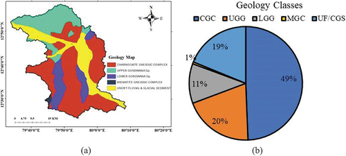
Figure 4(a) showed a geological map of the study area. The flow and existence of groundwater depend on porosity and permeability of rocks (Pande et al., 2022). Geologically, area fall under Archean to recent (age of formations) and showed a major percent of Charnockite Gneissic complex (Southern Granulite Terrain, Figure 4b) almost 49% of total area. For each geological unit, separate weights were assigned according to their groundwater prospects (Suganthi et al., 2013). For dolomites high weight was assigned followed by Undiff. Fluvial/Aeolian/Coastal & Glacial Sediments (UF/CGS), MGC (Migmatite Gneissic complex (Southern Granulite Terrain), LGG (Lower Gondwana Gp. (Talchir, Barakar, Raniganj, and Karharbari Fm.), UGG (Upper Gondwana Gp. (Yerrapalli, Terani, Sriperumpudurf, Kota, Maleri, Fm. Etc.), and CGC (Charnockite Gneissic Complex), respectively (Table 1).

Figure 4. (a) The geology map for study area, and (b) The geology class distribution graph of study area.

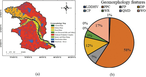
Geomorphology

Geomorphologic features gives a direct possibility about groundwater existence, flow and evolution (Machiwal et al., 2011). The hydro-geo-morphological features of the area were updated with Landsat 8 data. Based on the Geological Survey of India (GSI) digital data for study area, a total of six geomorphologic features (and two different types (WR and WO) have been identified (Figure 5(a)), such as: PPC Pediment Pediplain Complex (PPC) (Figure 5(a)), 58.4% of watershed area, Figure 5(b)), Waterbodies-Other (WO, 16.5%), Deltaic Plain (DP, 12.1%), Flood Plain (FP, 7.3%), Waterbody–River (WR, 4.6%), Low Dissected Denudational Hills and Valleys (LDDHV, 0.8%), QMD (Quarry and Mine Dump (QMD, 0.09%) and Coastal Plain (CP, 0.07%) (Figure 5). Geomorphic and morpho-structural study area advises neotectonic activity during the past period (UNDP, 1987). Among these morphological features, Coastal Plain (CP), Water body–River (WR) and Waterbodies-Other (WO) are lies under very good condition hence assigned as very high rank of 5, PPC and QMD are good (rank of 4). However, LDDHV, FP and DP are fall under poor condition for water potential zones hence assigned as very poor rank of 1 (low priority).

Figure 5. (a) The geomorphology map of study area, and (b) The geomorphology features distribution graph of study area.

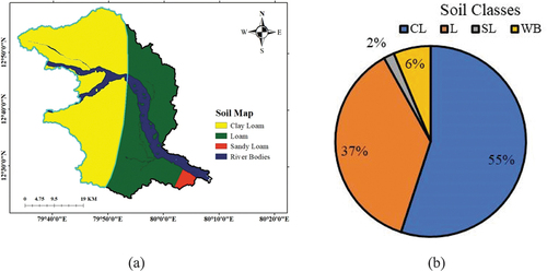
Soils

Soil map show mean soil texture or soil type (Figure 6(a)). Soil texture played a vital role in groundwater recharge and GWPZ. Runoff characteristics of any watershed are depend on water holding capacity of soil properties (porosity, thickness, etc.) and runoff characteristics have a good correlation with GWPZ. Zomlot et al. (2015) reported that groundwater recharge in loamy soils has a highest positive possibility which is an indication of more suitable area for groundwater potential. The area has clay loam (CL), loam (L) and sandy loamy (SL) soil and its distribution is as follows: 55%, 37% and 6% respectively (Figure 6(b)). In study area majority of soil is CL and L types based on FAO soil data.

Figure 6. (a) The soil map of study area, and (b) The soil classes distribution graph of study area.

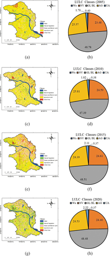
Land use/land cover (LULC)

LULC governed the infiltration or percolation and permeability process. The major LULC class was agriculture (AG, 25.57%), followed by natural vegetation (NV, 23.5%), grass/barren land (GL/BL, 48.8%), water body (W, 0.4%) and urban area (UA, 1.78%) in 2005 (Figure 7(a,b)). During 2010, the major LULC class was agriculture (AG, 25.81%), followed by natural vegetation (NV, 24.59%), grass/barren land (GL/BL, 47.39%), water body (W, 0.38%) and urban area (UA, 1.82%) which was increased 0.04% from last 5 year (Figure 7(c,d)). In 2015 LULC has slightly changed compared to 2010 (Figure 7(e,f)). LULC was reported as AG (24.39%), followed by NV (24.61%), GL/BL (48.51%), W (0.37%) and UA (2.11%). During the year 2020 LULC class wise distribution as follows: AG (24.53%), NV (24.40%), GL/BL, (48.48%), W (0.37%) and UA (2.22%; Figure 7(g,h)). The highest change was observed in AG class with respect to year 2005 (465.81 km²) to year 2020 (468.361 km²) almost 19.9 km² area has been reduced. However, NV has increased (17.5 km²) with respect to year 2005. Biological wreathing help in water percolation which results into enhanced groundwater level or improvement of water potential zones. The areal distribution of natural vegetation and scrub forests is as follows: 23.5% (2005), followed by 24.59% (2010), 24.61% (2015) and 24.40% (2020). The water percolation and infiltration rate within NV and around NV is higher therefore a high score (4) was assigned to NV class. Scrub/grass/barren lands have very shallow soils that are slightly also suitable for percolation and infiltration process rate, again groundwater potential of area will improve. Hence, a moderate score (2) was assigned to GL/BL class. AG (loose soils influence water to infiltrate to the subsurface) class is more favorable than GL/BL and UA area for percolation and recharge process. The good score of 3 was assigned to the AG class. The UA class has almost 100% of surface runoff with almost zero percent of infiltration and percolation rate and a very low score (1) was assigned to UA (Table 1).

Figure 7. (a) The LULC map of study area of 2005 (b) The LULC distribution (in %) of year 2005 (c) The LULC map of study area of 2010 (d) The LULC distribution (in %) of year 2005 (e) The LULC map of study area of 2015 (f) The LULC distribution (in %) of 2015 (g) The LULC map of study area of 2020, and (h) The LULC distribution (%) of 2020.

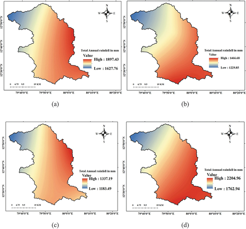
Rainfall

Rainfall is a vital component to assess potential zone of groundwater. Rainfall, infiltration and percolation are three factors which directly control groundwater table of an aquifer (Maity & Mandal, 2019). Das (2019) has found a good co-relationship between rainfall and groundwater table fluctuation. Considering this a score for rainfall was allotted as 1 to 5. The average annual rainfall is about 1213.3 mm and behavior is erratic. Based on average annual rainfall a distribution map (Figure. 8), has been categorized into five category (score is also 1 to 5), they are, less than 1627.76 mm or 1627.76 to 1708.13 mm, 1708.13 to 1761.01 mm, 1761.01 to 1803.31 mm, 1803.31 to 1841.38 mm, and 1841.38 to 1897.43 mm and score has been allotted as 1, 2, 3, 4 and 5, respectively (Table 1).

Figure 8. (a) The average annual rainfall distribution of 2005 (b) The average annual rainfall distribution of 2010 (c) The average annual rainfall distribution of 2015, and (d) The average annual rainfall distribution of 2020.

Slope information

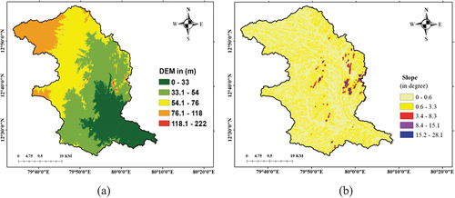
The spatial information of elevation is shown in Figure 9(a). Slope gradient directly impact over the infiltration and percolation process of rainfall (Figure 9(b)). Therefore, slope information can be used as one of the vital key for identification of GWPZs (Singh et al., 2018). Therefore, slope help to identify the infiltration and percolation rate of rainfall into ground, however, higher degree of slopes means a rapid runoff and negatively correlated with infiltration and percolation rate. Whereas, at level and gently sloping area, where rain water always flows on the surface with lower velocities and positively correlated with infiltration and percolation rate. The slope varies between 0 and 28.1° in the study area (Figure 9(b)). Flat slope area give more possibility infiltration and percolation process in comparison to the steep slope. This fact was considered while assigning the weightage or score for various slope classes. Watershed slope has been categorized into five classes. In study area a large part come under the nearly level slope (0° to 0.5°, Figure 9(b)) class which indicate toward the presence of good GWPZs (Pande et al., 2020). Based on Figure 9(b), cover with nearly level (0 to 0.5°, with highest score of 5 because of nearly level, which give more possibility of more infiltration and percolation process of rainfall with late runoff), very gently sloping (0.6 to 3.3°, with score of 4 because of late runoff), gently sloping (3.4 to 8.3°, with score of 3), moderate sloping (8.4 to 15.2°, with score of 2), and steep sloping (15.2 to 28.1°, with score of 1 because of higher degree of slope results of quick runoff which give almost zero present of infiltration and percolation process) and slope covers about 60.53%, 37.55%, 1%, 0.6% and 0.29% of the total area of watershed, respectively.

Figure 9. (a) The DEM of study area, and (b) The slope map of study area.

Weighted overlay analysis (WOA)

The WOA is a pixel based analysis technique. Different layers have different measurement units like rainfall layer in mm, DEM in meter, slope layer in degree, D_d in per kilometer (Table 1) and others. For WOA these all layers must be in same scale hence a score 1 to 5 was assigned to each layer. After assigning score, all layers at same index and now integrated into one. In a particular a raster has a value or score of 5 represents slopes of 0 to 0.5°, a score of 5 represents D_d of 1.2 to 2.13 km/km², a value of 5 represents soil type of loamy, a score of 5 represents water in LULC and a score of 5 represents rainfall of 1,841.38 to 1,897.43 mm. The high weighted value was considered as groundwater prospective area (Subba Rao et al., 2016).

Validation of GWPZ

The GWPZ map was validated using the existing wells data using Receiver Operating Characteristics (ROC) or Area Under the Curve (AUC) method (Naghibi et al., 2018). The wells data within the watershed were overlaid on GWPZ. In the graphical representations, the false positive rate (FPR) and the true-positive rate (TPR) values are representing in the X and Y axis, and it is denoted by equation 3 and 4. Value range of the ROC curve from 0.5 (or 50%, moderate) to 1.0 (or 100%, best). If the model unable to forecast the existences of the groundwater zones the AUC will be 0.5.

(3) $\mathrm{X}=\mathrm{FPR}=1-\frac{\mathrm{TN}}{\mathrm{TN}+\mathrm{FP}}$(3)

(4) $\mathrm{Y}=\mathrm{TPR}=1-\frac{\mathrm{TP}}{\mathrm{TP}+\mathrm{FN}}$(4)

Groundwater water potential zone (GPZ)

The GWPZ has been divided into five zones, a brief description in given in following sections:

Zone-I (Very Poor)

This zone has a steeper slope and high runoff hence a very low groundwater potential. Slope is a very steep 15.2 to 28.1° and this zone is located at northern and western part. It covers an area of 2.92% (or 55.81 km², Figure 10(b)), 3.14% (or 60.3 km², Figure 10(d)), 2.42% (or 46.28 km², Figure 10(f)), and 3.24% (or 61.89 km², Figure 10(h)) of total study area (1909.58 km²) during years 2005, 2010, 2015, and 2020, respectively.

Figure 10. (a) The GWPZ of 2005 (b) The distribution GWPZ 2005 c The GWPZ of 2010 (d) The distribution GWPZ 2010 (e) The GWPZ of 2015 (f) The distribution GWPZ 2015 (g) The GWPZ of 2020, and (h) The distribution GWPZ 2020.

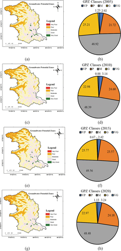
Zone – II (Poor, P)

In this zone slope ranges from 8.4–15.1°, such watershed area has D_d range of 0.20 to 0.51 km/km². This area also has clay loam soil and relief is also high. Therefore, zone-II also has few possibilities of groundwater occurrences. This area cover 21.72% (or 414.80 km², Figure 10(b)), 24.60% (or 469.82 km², Figure 10(d)), 23.57% (or 450.05 km², Figure 10(f)), and 24.18% (or 461.73 km², Figure 10(h)) of total area of watershed (1909.58 km²) during years 2005, 2010, 2015, and 2020, respectively. Spatial distribution of area is shown in GWPZ map for years 2005 (Figure 10(a)), 2010 (Figure 10(c)), 2015 (Figure 10(e)) and 2020 (Figure 10(g)).

Zone – III (Moderate, M)

The slope in zone-III ranges from 3.4–8.3°. It has an agriculture land of watershed. This area covers 934.19% (or 48.92 km², Figure 10(b)), 48.39% (or 923.98 km², Figure 10(d)), 49.56% (or 946.39 km², Figure 10(f)), and 48.48% (or 925.78 km², Figure 10(h)) of total area of watershed (1909.58 km²) during years 2005, 2010, 2015, and 2020, respectively. This is mainly due to gentle slope and fairly distributed loam soil and agriculture land with good capacity of infiltration and percolation. Spatial distribution of area is shown in GWPZ map for years 2005 (Figure 10(a)), 2010 (Figure 10(c)), 2015 (Figure 10(e)) and 2020 (Figure 10(g)) with accurate latitude and longitude. It has suitable groundwater availability but most of area comes in this zone from grass land/barren land and some part from agriculture also.

Zone – IV (Good, G)

This zone has good possibilities of water as slope ranges from 0.6–3.3° and Dd range of 0.83 to 1.19 km/km². In this zone most contribution of land from agriculture and natural vegetation and is easily bore able. It covers 25.1% (or 481.33 km², Figure 10(b)), 22.98% (or 438.91 km², Figure 10(d)), 23.77% (or 454 km², Figure 10(f)), and 22.97% (or 438.86 km², Figure 10(h)) of total area of watershed (1909.58 km²) during years 2005, 2010, 2015, and 2020, respectively. Spatial distribution of area is shown in GWPZ map for years 2005, 2010, 2015, and 2020, given by Figure 10(a), Figure 10(c), Figure 10(e) and Figure 10(g) respectively.

Zone–V (Very Good)

In this class GWPZ has favorable condition but major contribution of slope as it range of 0° to 0.5° and it has good groundwater occurrence. But very low area comes under this class. It may be due to eroded pediplain and agricultural land with high infiltration and percolation capacity. Moreover, during both monsoons, the study area receives very good amount of rainfall which drains these watershed therefore zone-V have a high potentiality of retaining groundwater. This excellent zones or class contribute covers 1.23% (or 23.45 km², Figure 10(b)), 0.88% (or 16.83 km², Figure 10(d)), 0.67% (or 12.86 km², Figure.10(f)), and 1.13% (or 21.64 km², Figure 10(h)) of total area of watershed (1909.58 km²) during years 2005, 2010, 2015, and 2020, respectively. Spatial distribution of this class is very few but near of water body.

Validation

The five years difference map of GWPZ were compared with a groundwater depth contour map for 2005, 2010, 2015, and 2020 locations of bore wells (Figure 11(a-g)). The good and moderate GWPZ, has reasonably flat water table and widely spaced contours. The much spread contours surrounded by closely spaced contours represent that the groundwater level is relatively flat. The total number 3 (3.7%), 4 (4.9%), 4 (4.9%) and 4 (4.9%) wells are located mostly in good potential zones (Figure.11(b-h)) during 2005, 2010, 2015, and 2020, respectively. However, 70 (85.4%), 60 (73.2%), 58 (70.7%), and 62 (75.6%) wells are come under the moderate potential zones (Figure 11(b-h)) during 2005, 2010, 2015, and 2020, respectively. We also found that wells total 9 (11%), 18 (22%), 20 (24.4%), and 16 (19.5%) wells come under the poor potential zone (Figure 11(b-h)) during 2005, 2010, 2015, and 2020, respectively.

Figure 11. (a) The GWPZ map of 2005 (b) The distribution GWPZ of 2005 (c) The GWPZ map of 2010 (d) The distribution GWPZ of 2010 (e) The GWPZ map of 2015 (f) The distribution of GWPZ in percentage 2015 (g) The GWPZ map of 2020, and (h) The distribution of GWPZ in percentage 2020.

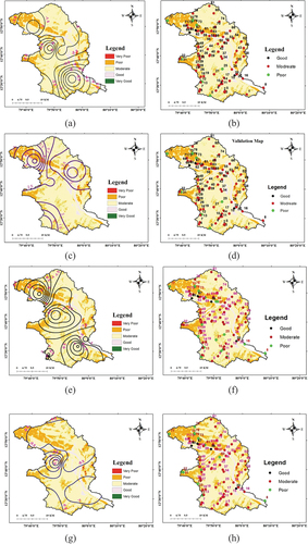
Total 82 location data was used for validation, majority of data falls on upper part and low in lower part of watershed respectively. Besides, due to uneven distribution of wells, preparation of the groundwater fluctuation was not reasonable. Therefore, the validity of the groundwater potential map was also performed by overlying the wells data on final map. The overlay analysis shows that only 5% (during 2005 to 2020) wells were fall on good zones. In study we also observed that during 2010 and 2015 moderate potential zones converged into poor category (Table 2) it is due to high exploration of groundwater and less rainfall or raising of drought condition. Almost each type of water conservation practices (plantation, rainwater harvesting structure, artificial recharge bore well, and water conservation structure, etc.) can be implementing in this category for development of groundwater resource.

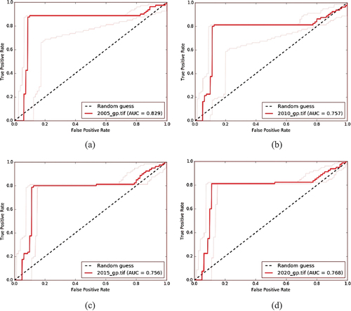
Accuracy of the GWPZ map was validated using ROC or AUC analysis with the existing 82 wells. During the ROC analysis the value of AUC for each five years interval and these were 0.829 (or 82% at a significance value of less than 0.001, Figure 12(a)), 0.757 (Figure 12(b)), 0.756 (Figure 12(c)) and 0.768 (or 76% at a significance value of less than 0.001, Figure 12(d)) for 2005, 2010, 2015, and 2020, respectively.

Figure 12. (a) The ROC curve for validation of predicted map 2005 (b) The ROC curve for validation of predicted map 2010 (c) The ROC curve for validation of predicted map 2015, and (d) The ROC curve for validation of predicted map 2020.

Conclusions

The GWPZ delineation was carried out using seven criteria in GIS platform. The GWPZ map was categorized into different classes and very poor-GWPZs have fall in clay loam with rocky soils and in very poor GWPZs the rooftop rainwater harvesting structures are recommended. The areas under poor-GWPZs are required a rigorous appropriate planning and management because a large area of watershed approx. (around) 24 km² area come under poor-GWPZs class. In such area small check dam and artificial recharge structure or bore well can be developed for improving groundwater resources. The medium-GWPZ category also covers a large part of watershed around 49% of total area of watershed. This category has a large area of watershed because some part of agriculture land and barren land are contributed in this category. The medium-GWPZ, has vast scope for implementation of groundwater resource improvements programs because barren land give the opportunity for it and for improving this category is required less efforts in comparison of poor-GWPZs category. Around 25% watershed area falls in good category. Moreover, present research work has good possibility to improve the irrigation facilities as well as agricultural productivity.

Disclosure statement

No potential conflict of interest was reported by the author(s).

References

- Agarwal, E., Agarwal, R., Garg, R. D., & Garg, P. K. (2013). Delineation of groundwater potential zone: An AHP/ANP approach. Journal of Earth System Science, 122(3), 887–898. https://doi.org/10.1007/s12040-013-0309-8
- Arabameri, A., Rezaei, K., Cerda, A., Lombardo, L., & Rodrigo-Comino, J. (2019). GIS-based groundwater potential mapping in Shahroud plain, Iran. A comparison among statistical (bivariate and multivariate), data mining and MCDM approaches. Science of the Total Environment, 658, 160–177. https://doi.org/10.1016/j.scitotenv.2018.12.115
- Chowdhury, A., Jha, M. K., & Chowdary, V. M. (2010). Delineation of groundwater recharge zones and identification of artificial recharge sites in West Medinipur district, West Bengal, using RS, GIS and MCDM techniques. Environmental Earth Sciences, 59(6), 1209–1222. https://doi.org/10.1007/s12665-009-0110-9
- Das, S. (2019). Comparison among influencing factor, frequency ratio, and analytical hierarchy process techniques for groundwater potential zonation in Vaitarna basin, Maharashtra, India. Groundwater for Sustainable Development, 8, 617–629. https://doi.org/10.1016/j.gsd.2019.03.003
- Das, N., & Mukhopadhyay, S. (2020). Application of multi-criteria decision making technique for the assessment of groundwater potential zones: A study on Birbhum district, West Bengal, India. Environment, Development and Sustainability, 22(2), 931–955. https://doi.org/10.1007/s10668-018-0227-7
- Fetter, C. W. (1994). Applied hydrogeology (3rd ed.). Macmillan College Publishing Company.
- Horton, R. E. (1932). Drainage-Basin characteristics. Transactions, American Geophysical Union, 13(1), 350–361. https://doi.org/10.1029/TR013i001p00350
- Jha, M. K., Chowdhury, A., Chowdary, V. M., & Peiffer, S. (2007). Groundwater management and development by integrated remote sensing and geographic information systems: Prospects and constraints. Water Resources Management, 21(2), 427–467. https://doi.org/10.1007/s11269-006-9024-4
- Kumar, M. G., Agarwal, A. K., & Bali, R. (2008). Delineation of potential sites for water harvesting structures using remote sensing and GIS. Journal of the Indian Society of Remote Sensing, 36(4), 323–334. https://doi.org/10.1007/s12524-008-0033-z
- Kumar N, Singh S Kumar and Pandey H K. (2018). Drainage morphometric analysis using open access earth observation datasets in a drought-affected part of Bundelkhand, India. Appl Geomat, 10(3), 173–189. https://doi.org/10.1007/s12518-018-0218-2
- Kumar N and Singh S Kumar. (2021). Soil erosion assessment using earth observation data in a trans-boundary river basin. Nat Hazards, 107(1), 1–34. https://doi.org/10.1007/s11069-021-04571-6
- Kumar, M., Singh, S. K., Kundu, A., Tyagi, K., Menon, J., Frederick, A., Lal, D., & Lal, D. (2022). GIS-based multi-criteria approach to delineate groundwater prospect zone and its sensitivity analysis. Applied Water Science, 12(4), 1–14. https://doi.org/10.1007/s13201-022-01585-8
- Kumar Pradhan R, Srivastava P K, Maurya S, Kumar Singh S and Patel D P. (2020). Integrated framework for soil and water conservation in Kosi River Basin. Geocarto International, 35(4), 391–410. https://doi.org/10.1080/10106049.2018.1520921
- Machiwal, D., Jha, M. K., & Mal, B. C. (2011). Assessment of groundwater potential in a semi-arid region of India using remote sensing, GIS and MCDM techniques. Water Resources Management, 25(5), 1359–1386. https://doi.org/10.1007/s11269-010-9749-y
- Magesh, N. S., Chandrasekar, N., & Soundranayagam, J. P. (2012). Delineation of groundwater potential zones in Theni district, Tamil Nadu, using remote sensing, GIS and MIF techniques. Geoscience Frontiers, 3(2), 189–196. https://doi.org/10.1016/j.gsf.2011.10.007
- Maity, D. K., & Mandal, S. (2019). Identification of groundwater potential zones of the Kumari river basin, India: An RS & GIS based semi-quantitative approach. Environment, Development and Sustainability, 21(2), 1013–1034. https://doi.org/10.1007/s10668-017-0072-0
- Mohamed, M. M., & Elmahdy, S. I. (2017). Fuzzy logic and multi-criteria methods for groundwater potentiality mapping at Al Fo’ah area, the United Arab Emirates (UAE): An integrated approach. Geocarto International, 32(10), 1120–1138. https://doi.org/10.1080/10106049.2016.1195884
- Mondal, N. C., Rao, V. A., Singh, V. S., & Sarwade, D. V. (2008). Delineation of concealed lineaments using electrical resistivity imaging in granitic terrain. Current Science, 94(8), 1023–1030.
- Murmu, P., Kumar, M., Lal, D., Sonker, I., & Singh, S. K. (2019). Delineation of groundwater potential zones using geospatial techniques and analytical hierarchy process in Dumka district, Jharkhand, India. Groundwater for Sustainable Development, 9, 100239. https://doi.org/10.1016/j.gsd.2019.100239
- Nagarajan, M., & Singh, S. (2009). Assessment of groundwater potential zones using GIS technique. Journal of the Indian Society of Remote Sensing, 37(1), 69–77. https://doi.org/10.1007/s12524-009-0012-z
- Naghibi, S. A., Pourghasemi, H. R., & Abbaspour, K. (2018). A comparison between ten advanced and soft computing models for groundwater qanat potential assessment in Iran using R and GIS. Theoretical and Applied Climatology, 131(3–4), 967–984. https://doi.org/10.1007/s00704-016-2022-4
- Pande, C. B., Moharir, K. N., Singh, S. K., & Varade, A. M. (2020). An integrated approach to delineate the groundwater potential zones in Devdari watershed area of Akola district, Maharashtra, Central India. Environment, Development and Sustainability, 22(5), 4867–4887. https://doi.org/10.1007/s10668-019-00409-1
- Pande, C. B., Moharir, K. N., Panneerselvam, B., Singh, S. K., Elbeltagi, A., Pham, Q. B., Rajesh, J., & Rajesh, J. (2021). Delineation of groundwater potential zones for sustainable development and planning using analytical hierarchy process (AHP), and MIF techniques. Applied Water Science, 11(12), 1–20. https://doi.org/10.1007/s13201-021-01522-1
- Pande, C. B., Moharir, K. N., Singh, S. K., Elbeltagi, A., Pham, Q. B., Panneerselvam, B., Kouadri, S., & Kouadri, S. (2022). Groundwater flow modeling in the basaltic hard rock area of Maharashtra, India. Applied Water Science, 12(1), 1–14. https://doi.org/10.1007/s13201-021-01525-y
- Pandey, H. K., Singh, V. K., Singh, S. K., Douzals, J.-P., Guibal, R., Grimbuhler, S., Grünberger, O., Lissalde, S., Mazella, N., Samouëlian, A., & Simon, S. (2022). Multi-criteria decision making and Dempster-Shafer model–based delineation of groundwater prospect zones from a semi-arid environment. Environmental Science and Pollution Research, 29(1), 1–19. https://doi.org/10.1007/s11356-021-17416-3
- Rawat, K. S., Jeyakumar, L., Singh, S. K., & Tripathi, V. K. (2019). Appraisal of groundwater with special reference to nitrate using statistical index approach. Groundwater for Sustainable Development, 8, 49–58. https://doi.org/10.1016/j.gsd.2018.07.006
- Saaty TL (1980) The analytic hierarchy process. McGraw Hill, New York
- Singh, S., Singh, C., & Mukherjee, S. (2010). Impact of land-use and land-cover change on groundwater quality in the Lower Shiwalik hills: A remote sensing and GIS based approach. Open Geosciences, 2(2), 124–131. https://doi.org/10.2478/v10085-010-0003-x
- Singh, L. K., Jha, M. K., & Chowdary, V. M. (2018). Assessing the accuracy of GIS-based multi-criteria decision analysis approaches for mapping groundwater potential. Ecological Indicators, 91, 24–37. https://doi.org/10.1016/j.ecolind.2018.03.070
- Singh VG., & Singh SK (2022). Analysis of geo-morphometric and topo-hydrological indices using COP-DEM: a case study of Betwa River Basin, Central India. Geology, Ecology, and Landscapes. https://doi.org/10.1080/24749508.2022.2097376
- Subba Rao, N., & Prathap Reddy, R. (2004). Geoenvironmental appraisal in a developing urban area. Environmental Geology, 47(1), 20–29. https://doi.org/10.1007/s00254-004-1122-0
- Subba Rao, N. (2006). Groundwater potential index in a crystalline terrain using remote sensing data. Environmental Geology, 50(7), 1057–1067. https://doi.org/10.1007/s00254-006-0280-7
- Subba Rao, N. (2009). A numerical scheme for groundwater development in a watershed basin of basement terrain: A case study from India. Hydrogeology Journal, 17(2), 379–396. https://doi.org/10.1007/s10040-008-0402-2
- Subba Rao, N. (2011). Guidelines for success of well site selections. Current Science, 100(8), 1119–1120.
- Subba Rao, N., Moeen, S., Surya Rao, P., Dinakar, A., Nageswara Rao, P. V., Sunitha, B., Rudra, D., & Srinivasu, N. (2016). Morphometric approach using remote sensing and GIS in watershed management. Journal of Applied Geochemistry, 18(1), 45–56.
- Subba Rao, N., Sakram, G., & Rashmirekha, D. (2022). Deciphering artificial groundwater recharge suitability zones in the agricultural area of a river basin in Andhra Pradesh, India using geospatial techniques and analytical hierarchical process method. Catena, 212, 106085. https://doi.org/10.1016/j.catena.2022.106085
- Suganthi, S., Elango, L., & Subramanian, S. K. (2013). Groundwater potential zonation by remote sensing and gis techniques and its relation to the groundwater level in the coastal part of the Arani and Koratalai River Basin, Southern India. Earth Sciences Research Journal, 17(2), 87–95. http://www.scielo.org.co/pdf/esrj/v17n2/v17n2a2.pdf
- Suja Rose, R. S., & Krishnan, N. (2009). Spatial analysis of groundwater potential using remote sensing and GIS in the Kanyakumari and Nambiyar basins, India. Journal of the Indian Society of Remote Sensing, 37(4), 681–692. https://doi.org/10.1007/s12524-009-0058-y
- Thomas, A., Sharma, P. K., Sharma, M. K., & Sood, A. (1999). Hydrogeomorphological mapping in assessing ground water by using remote sensing data A case study in Lehra gaga block, Sangrur district, Punjab. Journal of the Indian Society of Remote Sensing, 27(1), 31–42. https://doi.org/10.1007/BF02990773
- Tweed, S. O., Leblanc, M., Webb, J. A., & Lubczynski, M. W. (2007). Remote sensing and GIS for mapping groundwater recharge and discharge areas in salinity prone catchments, southeastern Australia. Hydrogeology Journal, 15(1), 75–96. https://doi.org/10.1007/s10040-006-0129-x
- Yadav S Kumar, Singh S Kumar, Gupta M and Srivastava P K. (2014). Morphometric analysis of Upper Tons basin from Northern Foreland of Peninsular India using CARTOSAT satellite and GIS. Geocarto International, 29(8), 895–914. https://doi.org/10.1080/10106049.2013.868043
- Yadav S Kumar, Dubey A, Szilard S and Singh S Kumar. (2018). Prioritisation of sub-watersheds based on earth observation data of agricultural dominated northern river basin of India. Geocarto International, 33(4), 339–356. https://doi.org/10.1080/10106049.2016.1265592
- Yadav S Kumar, Dubey A, Singh S Kumar and Yadav D. (2020). Spatial regionalisation of morphometric characteristics of mini watershed of Northern Foreland of Peninsular India. Arab J Geosci, 13(12). https://doi.org/10.1007/s12517-020-05365-z
- Zolekar, R. B., & Bhagat, V. S. (2015). Multi-criteria land suitability analysis for agriculture in hilly zone: Remote sensing and GIS approach. Computers and Electronics in Agriculture, 118, 300–321. https://doi.org/10.1016/j.compag.2015.09.016
- Zomlot, Z., Verbeiren, B., Huysmans, M., & Batelaan, O. (2015). Spatial distribution of groundwater recharge and base flow: Assessment of controlling factors. Journal of Hydrology: Regional Studies, 4, 349–368. https://doi.org/10.1016/j.ejrh.2015.07.005