Prediction of forest aboveground biomass using an integrated approach of space-based parameters, and forest inventory data

ABSTRACT

Forests contribute significantly in mitigating the effects of climate change by sequestering atmospheric carbon in biomass and soil. To comprehend carbon stock and sequestration, forest degradation, and climate change mitigation, precise calculation biomass is needed. The present study in Arunachal Pradesh, Northeast India, used Landsat OLI spectral variables, land surface temperature, and field inventory data to estimate aboveground biomass (AGB) and carbon stock in selected forest types. The stepwise multilinear regression model was developed using Landsat-derived spectral data, land surface temperature, and soil moisture The stand density varies from 122 individual ha⁻¹ to 833 individual ha⁻¹ . The estimated AGB density varies from 2.64 t ha⁻¹ to 534.21 t ha⁻¹ among the sample plots. The mean land surface temperature was 14.41°C. The predictive integrated model showed that the mean AGB ranged from 9.45 t ha⁻¹ to 330 t ha⁻¹ and dense forest recorded the maximum mean AGB (239.34 t ha⁻¹). Akaike information criteria (AIC) and Bayesian information criteria (BIC) were utilised to evaluate the predictive model, and the AIC (176.13) and BIC (184.58) were omparatively lower than other regression models.To evaluate the accuracy of the integrated model (IM), the linear regression was performed between the predicted and observed AGB. The findings of the study will be useful in formulating site-specific suitable management plan.

KEYWORDS:

• Spectral variables
• regression analysis
• biomass
• Northeast India
• Land use

1. Introduction

The forest ecosystem has an indispensable contribution to the global carbon (C) cycle and is regarded as the largest carbon sink, which removes around 25–33% of the anthropogenic greenhouse gas (GHG) emission from the atmosphere (Le Quéré et al., 2016). Forest stores a considerable amount of forest carbon (70–90%) in aboveground biomass (AGB) (S. Chen et al., 2019) and a large portion of atmospheric carbon dioxide (CO₂) in terrestrial land and soil (Motlagh et al., 2018). Besides climate change mitigation, the forest nourishes numerous ecosystem services and is an indispensable component of earth’s energy cycle. The forest biomass is a crucial parameter to describe the structure and function of the forest ecosystem (Y. Li et al., 2020). Forest covert the atmospheric carbon and is stored in AGB, belowground biomass, dead organic matter, and soil organic matter (Ramachandra & Bharath, 2020). The forest ecosystem captures about 40% of terrestrial carbon and 50% of net ecosystem productivity (McGarvey et al., 2015). Annually, about 30% of the global anthropogenic CO₂ emissions (2 Pg C yr⁻¹) from the atmosphere sequestered by the forest and soil (Achat et al., 2006; Lal, 2005). The extent of land use change, anthropogenic pressure, disturbances, and climate change have affected the carbon capture, storage, and retention in forest and soil carbon pools. Further, the landuse land cover (LULC) changes induced forest ecosystem has been modifying the forest structure that increases the forest fragmentation, loss of biodiversity, biogeochemical cycle alteration, and hydrological services (Armenteras et al., 2019; Ramachandra & Bharath, 2019).

As the Intergovernmental Panel on Climate Change (IPCC) Fifth Assessment Report, deforestation stands second in the list of largest contributors of carbon dioxide (CO₂) emissions (Ciais et al., 2014). Deforestation and land degradation account for 20–25% of anthropogenic carbon emissions (Pachauri & Reisinger, 2007; Ramachandra & Bharath, 2019) hence influencing regional climate patterns including hydrogeological regime alternation. The forest cover loss has altered the local rainfall regime due to alternation in the pattern of thermodynamic and mesoscale circulation processes (Lawrence & Vandecar, 2015), which have extreme weather consequences afterwards. Further, the large and intact forest through their leaves, leaf area and canopy coverage transferring sensible heat to latent heat, which alter the wind dynamics and hence rainfall events increased (Ramachandra & Bharath, 2020). The deforestation causes lower evapotranspiration across the region, which has the consequence of delayed rainfall with low periodicity of rainfall with longer dry conditions (Debortoli et al., 2017). The deforestation may lead to biophysical alternation in plants through altered micro-climatic condition along with raising air and land surface temperature (LST) (Ramachandra et al., 2018). The increase in temperature has an upward trend in plant water demand leading to loss of canopy, microflora, microclimate change as well as an increase in the number of forest fire (Ramachandra & Bharath, 2019).

The forest biomass combustion and dead plant material decomposition due to deforestation and forest degradation have accelerated the atmospheric GHG emission particularly in developing countries (Pearson et al., 2017; Ramankutty et al., 2007). The terrestrial carbon cycle and carbon sequestration during the process of plant growth remains least affected aspect of the global carbon cycle (Le Quéré et al., 2018). Reducing emissions from deforestation and degradation (REDD) devised mechanisms to implement the forest monitoring system that needs primarily the forest carbon stock estimation (GOFC-GOLD, 2014; UNFCCC, 2009; UN-REDD, 2011) through integrated approach of field-based data and earth observatory data. Besides forest degradation and LULC change, various terrain parameters (slope, aspect and elevation) also have significant influence on forest composition, micro climate, solar radiation and moisture condition at different hill slopes of mountainous forests (Holland & Steyn, 1975; Måren et al., 2015; Sharma et al., 2010; Yadav & Gupta, 2006). The forest carbon stock estimation primarily depends on various carbon pool such as AGB, BGB, litter biomass, deadwood and soil organic carbon (SOC) (IPCC, 2006). However, the AGB alone has contributed about 50% to the carbon stock (Goetz & Dubayah, 2011).

There are two major approaches to estimate the forest AGB viz. destructive and non-destructive approach. The former is the most accurate and reliable method of AGB estimation. However, it fails when there was data belonging to large area coverage (Qureshi et al., 2012; Stovall et al., 2017). Therefore, the later is the most accepted approach of AGB estimation using allometric equations (Brown & Lugo, 1992; Chave et al., 2005, 2014). In the last two decades, the remote sensing (RS) technology became the most preferred approach and enables researchers to get large scale real-time synoptic view of vegetation conditions (Du et al., 2014; Tang et al., 2016). However, to estimate the more precise regional AGB, the RS technology depends on fine scale filed inventory data. Therefore, integrating field inventory data and RS technology has now been widely preferred in AGB estimation (Jiang et al., 2021; C. Li et al., 2019; Lu, 2006; Ravindranath et al., 2008; Tang et al., 2016). Several researcher have used data like MODIS (Pandey et al., 2019), Landsat TM (Deka et al., 2015; Günlü et al., 2014), Landsat ETM+ (Shen et al., 2020; Zheng et al., 2004), Landsat OLI (Bordoloi et al., 2022; Kashung et al., 2018), IKONOS (Thenkabail et al., 2004), WorldView-2 (Eckert, 2012), RADAR (Gunawardena et al., 2015), Sentinel-1A (Y. Li et al., 2020; Norovsuren et al., 2020) to study the forest AGB.

Many authors have reported the significance of crucial variables to develop a model that estimates the forest AGB (S. Chen et al., 2019; Yu et al., 2019). Normalized difference vegetation index (NDVI), Soil-adjusted vegetation index (SAVI) and Enhanced vegetation index (EVI), Atmospheric resistant vegetation index (ARVI) were most widely used approaches (Bordoloi et al., 2022; Kashung et al., 2018; Shen et al., 2020). Besides above, the digital elevation model (DEM) derived topographic variables like slope, aspect can also be utilized as variables for AGB estimation model. Some researchers have used environmental parameters like temperature, land surface temperature, soil moisture in forest parameter estimation (Jiang et al., 2021; Zarco-Tejada et al., 2018). The satellite-derived land surface temperature from the thermal infrared sensor (TIRS) of Landsat improves the accuracy in estimating leaf area index (LAI) (Neinavaz et al., 2019) while its use in AGB estimation needs to be evaluated. The use of large number of variables can be time-consuming, estimation erroneous and render the applicability and interpretability of the model (Yu et al., 2019). Hence, the suitable variables combination selection is crucial for the AGB estimation. Numerous algorithms have been used by the researcher, among them classical statistical linear regression algorithm was the most widely used algorithm due its simplicity nature (C. Li et al., 2019; Lu et al., 2014; Sarker & Nichol, 2011). The linear relationship analysis used RS based spectral variables and the field inventory data. Hence a stepwise multi-linear regression approach was used in the present study. The objective of the study is to estimate and predict the biomass stock of different land-use sectors of the region in connection to climate change scenarios. The study will assess the region’s biomass stock using in situ measurements from sample plots and pixel-based RS derived spectral variables, land surface temperature and soil moisture to simulate the spatial biomass density.

2. Materials and methods

2.1 Study area

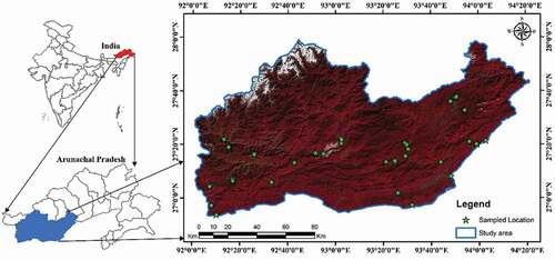
The present study was carried out in four western districts of Arunachal Pradesh (West Kameng, East Kameng, Papum pare and Lower Subansiri) which were spread in the mountainous forest of eastern Himalayas. The study region spreads over an area of 17,384 km² and lies 26°52’ to 29°59’ N latitude and 92°01’ to 94°22’ E longitude. The climate of the state varies sharply with changes in latitude and elevation. The areas at very high elevation in the upper Himalayas close to the Tibetan border enjoy an alpine climate while below this region it is temperate. The areas at the sub-Himalayan experience humid subtropical climate along with hot summers and mild winters. The average mean maximum and minimum temperature varied between 29.5°C and 17.7°C in subtropical regions and 21.4°C and 2.4°C in cold humid regions and the foothills and plains experience higher temperatures. The area is rich in biodiversity including the treasure of germplasm for species of food, medicinal, bamboo and cane, orchids, wild animal, and other life forms. As there was a paucity of data on carbon sequestration in the state, it became crucial to carry out such studies to estimate the AGB, carbon pool and carbon sequestration of the region (Figure 1).

Figure 1. Map shows the location of Sample plot in the study area.

2.2 Satellite data acquisition

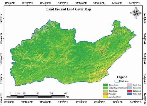
In the present study, cloud-free Landsat OLI optical RS data for the year 2018 and 2019 and Advanced space-borne thermal emission radiometer (ASTER) elevation data were selected and downloaded from Earth Explorer (https://earthexplorer.usgs.gov). In Landsat OLI data, the blue, green, red, near-infrared band, and thermal infrared band were used in the analysis. All the imageries were co-registered to a common UTM (Universal Transversal Mercator) projection system with WGS 84 datum (Zone 46). The top of atmospheric (TOA) reflectance correction was applied the imageries by following the radiometric correction method as per Landsat 8 user handbook (Zanter, 2019). Additionally, because of the presence of complex terrain conditions along with dense forest cover in the region, it was precautionary to apply topographic illumination correction, hence an improved cosine correction method (Civco, 1989) was applied. The ASTER DEM data with 30 m resolution was used for topographic correction. The DEM images were re-sampled to Landsat OLI pixel size by the nearest neighbourhood transformation (Wu et al., 2016). For the forest inventory process, unsupervised classification approach was done. The satellite image of the study area categorized into nine land use land cover categories viz. dense forest, moderately dense forest, open forest, plantation, agriculture land, settlement, sandy area, snow areas, and water bodies (Figure 2).

Figure 2. Map shows the Land use land cover of the study area.

2.3 Forest inventory data collection

The selection of permanent sample plot was based on forest density class. To find out the different forest density classes, the classified land use map was used, and it showed dense forest, moderately dense forest, open forest, plantation among the major land use sectors in major agro-climatic zones. In each of the zones and major land use sectors, sampling plots were randomly selected in replicates. The forest inventory was done by establishing 61 number of sample plot of 31.6 m x 31.6 m (0.1 ha) as per standard layout. The sample quadrats were chosen on the basis of stratified random sampling approach and representative sites covering dense to sparse vegetation cover. Tree structural parameters like species, girth at breast height (GBH), height of the all the trees ≥ 30 cm girth at breast height (at 1.37 m from the base) were measured. The measuring tape, clinometer was used to measure the GBH and the height of plant species respectively. Further, GPS records were also taken for each plot. Forest inventory data were collected for a period of two years (2018–2019) and among 61 permanent plots, 14 number of plots sampled in dense forest (DF) and moderately dense forest (MDF) each, 20 plots in open forest (OF) and 13 plots in plantation (PL). Based on the tree DBH and height, the plot based AGB was calculated for trees having girth ≥ 30 cm at girth breast height (1.37 m) by applying the generalized allometric equation for the north-eastern region of India proposed by Nath et al. (2019), which is based on stem diameter, height, and wood density of the species.

2.4 Satellite-based spectral variables

The Landsat OLI spectral variables (SV) (Table 1) include difference vegetation index (DVI) which is a simple difference between near-infrared (NIR) and red (R) band ratio, normalized difference vegetation index (NDVI) which is the ratio of NIR and R bands, atmospheric resistant vegetation indices (ARVI) which uses three-band ratio to minimize the atmospheric scattering effect. Soil adjusted vegetation index (SAVI) minimizes soil brightness effects in the satellite image, and enhanced vegetation index (EVI) is the complex index and high sensitivity to high AGB region as it eliminates the aerosol influence and canopy background effect. Hence, these vegetation indices were incorporated to analyze the best relationship between the AGB and vegetation indices.

Table 1. Spectral variables used spatial mapping of biomass and carbon.

Vegetation Indices	Expression	Author
NDVI	$NDVI=\left(NIR-R\right)/\left(NIR+R\right)$	Rouse et al. (1974)
SAVI	$SAVI=\left[\left(NIR-R\right)/\left(NIR+R+L\right)\right]\left(1+L\right)$Where L = 0.5 for intermediated vegetation cover	Huete (1988)
ARVI	$ARVI=\left(NIR-RB\right)/\left(NIR+RB\right)$	Kaufman & Tanre, 1992
EVI	$EVI=G\ast \left(NIR-R\right)/\left(NIR+C_{1}R-C_{2}B+L\hspace{0.17em}\right)$Where: C1 = 6; C2 = 7.5; L = 1; G = 2.5	Liu and Huete (1995)

2.5 Forest biomass and carbon calculation

The non-destructive approach was used to estimate the forest AGB. Though the Forest Survey of India (FSI), have developed many species-specific allometric equations to estimate the tree AGB (FSI, 1996), however, there was a paucity of the allometric equation for many local species available in the study area. Hence, the generalized allometric equation developed by Nath et al. (2019) for the northeast India region was used in the present study. To estimate forest carbon stock a conversion factor of 0.55 was used (MacDicken, 1997).

2.6 Satellite-based LST and soil moisture estimation

The cloud-free Landsat 8 satellite imageries of the year 2018 to 2019 covering the study area were acquired from the Earth explorer. The Landsat 8 satellite has on boarded two different sensors, the operational land imager (OLI) and the Thermal infrared sensor (TIRS) having different resolution. The T1-level imageries having the radiometric correction and geometric correction were acquired. However, two prerequisite processes, the radiometric calibration and atmospheric correction were applied as per Landsat 8 manual (Zanter, 2019) to the all the imageries to get high quality and accurate image information. The automated algorithm imageries (Avdan & Jovanovska, 2016; Sobrino et al., 2004) was used in LST retrieval from Landsat 8. Among the available bands, Band 10 (TIR), Band 4 (RED), and Band 5 (NIR) were used in LST retrieval. The TIR band was used to derive brightness temperature, whereas the RED and NIR band was used in NDVI determination. The brightness temperature (BT) was obtained from the TIRS band using the thermal constant provided in the image metadata file. Following the NDVI, the land surface emissivity (LSE) was calculated, which was the most essential aspect of LST retrieval.

For the global climate change and large-scale hydrological cycles, the soil moisture (S_m) is regarded as important influencing factors (J. Chen et al., 2011). The retrieval of S_m was done by using the temperature vegetation dryness index (TVDI). The TVDI derived by using triangle method (Przeździecki et al., 2017; Sandholt et al., 2002), which utilized the NDVI and LST as influencing factor for S_m retrieval. To determine TVDI, dry edge (low evapotranspiration) and wet edge (maximum evapotranspiration) are the two crucial variables. To determine the dry and wet edge from triangle method, for each dry and wet edge, the maximum and lowest LST values were chosen from the pixel-based NDVI. As per J. Chen et al. (2011), the pixels having NDVI between 0.2–0.3 were chosen for dry edge calculation. The equation for TDVI is as follows.

$TDVI=\frac{LST-LS{T}_{min}}{LS{T}_{max}-LS{T}_{min}}$

Where:

$LS{T}_{min}$ is the minimum surface temperature for given pixel for wet edge and modelled using equation ($LS{T}_{min}$ = a_min + b_min*NDVI) in the triangle, where a_min and b_minare regression parameters for the wet edge (Table 2).

Table 2. TDVI retrieval parameter for Soil moisture retrieval.

Parameter	Slope	Intercept
Dry Edge	amin = −53.73	bmin = 35.56
Wet Edge	amax = 6.96	bmax = 10.034

$LS{T}_{max}$ is the maximum surface temperature for given pixel for wet edge and modelled using equation ($LS{T}_{max}$ = a_max + b_max*NDVI) in the triangle, where a_max and b_maxare regression parameters for the dry edge (Table 2). The linear regression analysis was carried out between the plot-based volumetric moisture content and the plot-based TDVI values to get the best fit model for S_m estimation of the study area.

2.7 Development of forest AGB model and evaluation

The RS-based SVs, and plot based AGB were taken into account to model the forest AGB of the study area. In the present study, the satellite data derived spectral variables like NDVI, SAVI, ARVI, EVI and physical variables like LST and S_m were evaluated to find out their linear relationships with plot based AGB of each land use sector (Table 2). The sampled plot’s locations were overlaid on different SVs, gridded LST, and S_m data to derive corresponding values of each sampled plot. The four most widely used vegetation indices (VIs) associated with RS based change detection and biomass estimation were used. The tested VIs includes NDVI, which was the ratio of complementary reflectance between the red and NIR spectral bands due to chlorophyll pigments and leaf cellular structure respectively (Powell et al., 2010), the SAVI, although similar to the NDVI but have an improvement in terms of the soil brightness correction factor (Huete, 1988) and the ARVI, which was self-correcting indices for both soil and atmosphere reflectance and minimizes both soil and atmospheric noises (Kaufman & Tanre, 1992).

As the current study area have complex landform feature along with different agro-ecological zone, it is quite difficult to characterize the precise estimation of AGB. Therefore, a statistical correlation was developed between LST, S_m, and VIs with the field-based AGB of each land-use sector. The plot based AGB was assessed against the satellite derived pixel based selected variables of the sampled location. To assess the same, the linear relationship between the variables and AGB was performed to get best relationship of the model. A multiple regression analysis approach was used for modelling the AGB, which was further validated.

For the AGB modelling, researchers have used numerous approaches like linear regression approach (Calvao & Palmeirim, 2004; Ren & Zhou, 2014), multi-regression approach (Askar et al., 2018; Eckert, 2012; Sarker & Nichol, 2011), non-linear regression (Santos et al., 2003), non-parametric model (Urbazaev et al., 2016), artificial neural network (Dong et al., 2020). In the present study, we have applied stepwise multi-linear regression analysis for assessing the relationship between AGB, spectral variables, LST and S_m. The multi-linear regression approach some time may lead to multicollinearity and overfitting in analysis hence to overcome this most widely used statistical parameter like Pearson correlation (r), root mean square error (RMSE), coefficient of determination (R²) and p – level were applied. The best fit model for AGB prediction was done based on high r and high R² values. A step wise linear regression method was employed for modelling AGB using Origin software. Further to confirm the reliability of the model, R², RMSE, multicollinearity of variables, the variance inflation factor {VIF = VIFj = 1/ (1-R_j²)} were determined. To indicate multicollinearity problem, VIF value greater than 10 (Askar et al., 2018; Sarker & Nichol, 2011) were determined. Further, Akaike information criteria (AIC; Akaike, 1974) and Bayesian information criteria (BIC; Aho et al., 2014) were used in the suitable model selection process. The selection of model was done based on observed smallest AIC and BIC values.

3. Result

3.1 Tree density, aboveground biomass, and carbon stock

From the study, it was observed that the mean density varies from 122 individual ha⁻¹ to 833 individual ha⁻¹ among the sample plots. Among the forest types, plantation has recorded maximum tree density of 609 individual ha⁻¹ followed by the dense forest (563 individual ha⁻¹), moderately dense forest (517 individual ha⁻¹) and open forest (343 individual ha⁻¹). The AGB density varies among the different forest types, and it ranges from 2.64 t ha⁻¹ to 534.21 t ha⁻¹ among the sample plots. The dense forest have recorded the maximum AGB of 279.41 t ha⁻¹ followed by the moderately dense forest (161.16 t ha⁻¹), plantation (88.99 t ha⁻¹) and open forest (61.86 t ha⁻¹) (Table 3).

Table 3. Observed AGB of the sample plot in the study area.

Forest Type	Plot number	Mean density	Mean AGB	Range	Standard Deviation
DF	14	563	279.41	156.06–534.21	107.84
MDF	14	517	161.16	96.56–235.69	43.99
OF	20	343	61.86	2.64–162.70	43.15
PL	13	609	88.99	21.07–221-62	58.67
Total	61	482	147.85	2.64–534.21	107.03

3.2 LST and Soil moisture estimation

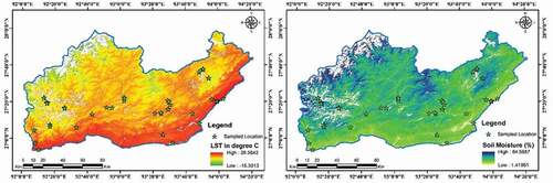
The mean LST for the study area was 14.41°C, however it varied among the different forest types. The mean LST observed for DF was 10.19°C, MDF (14.34°C), OF (16.16°C), and PL (16.32°C). The S_m of the study area was estimated based on regression model developed between TDVI and field based volumetric soil moisture content of the sample plot. The developed model (S_m = −103.31*TDVI+147.38, R² = 0.70) showed that the mean S_m of the study area was 30.64%, however it ranged between 1.41 and 84.56% (Figure 3).

Figure 3. Land surface temperature and soil moisture of the study area.

3.3 Optimum variable selection

The statistical analysis of individual SVs with the AGB was done by linear regression analysis and it was evident that the correlation coefficient (R²) obtained between NDVI and AGB was 0.60 with RMSE of 36.50 t ha⁻¹. Similarly, for the SAVI (R² = 0.61, RMSE = 35.52 t ha⁻¹), ARVI (R² = 0.65, RMSE = 32.37 t ha⁻¹), and for EVI (R² = 0.60, RMSE = 36.53 t ha⁻¹). However, the linear regression analysis of LST with AGB showed R² = 0.61, RMSE = 35.97 t ha⁻¹ and that of S_m with the AGB resulted R² = 0.62, RMSE = 34.63 t ha⁻¹ (Table 4).

Table 4. Statistical analysis of stepwise multilinear regression of AGB with variables.

Variables	R^2	r	RMSE	p-value	VIF
NDVI	0.60	0.77	36.51	0.00	2.52
SAVI	0.61	0.78	35.52	0.00	2.59
ARVI	0.64	0.80	32.36	0.0002	2.84
EVI	0.60	0.77	36.53	0.00	2.52
LST	0.61	0.78	35.97	0.00	2.56
Sm	0.62	0.79	34.63	0.00	2.66
Integrated Model (IM)	0.82	0.90	17.09	0.00	5.67

IM = SAVI + ARVI + LST + S_m

3.4 Modelling of AGB

The stepwise multi-linear regression analysis was used to select appropriate variables for predictive AGB model development. This was done by anlysing the resultant R², RMSE and VIF observed from linear relationship analysis individual variables with AGB. The selection of the variable’s combination was based on the minimum RMSE of the model. The statistical relationship of individual SVs, then combining all the SVs, and finally combining the LST and S_m with the SVs is presented in Table 4.

The linear regression analysis of field based AGB and individual variables of the study area is shown in Table 4. The correlation coefficient R² ranged between 0.60 and 0.64 whereas the Pearson’s r varied between 0.77 and 0.80. Among the selected SVs, the ARVI have shown better correlation (r = 0.80, R² = 0.64). It was evident that all the selected variables have shown significant and positive correlation with AGB. Further, the predictive AGB model derived from stepwise multi- linear regression technique has been expressed as follows:

$AGB=23.71\ast SAVI+15.62\ast ARVI-0.72\ast LST+0.34\ast SM-4.23$

The developed predictive model derived using SVs, LST, and S_m have shown R² = 0.82, p < 0.05. The RMSE of the model was observed to be 17.09 t ha⁻¹.

3.5 Spatial AGB and carbon density mapping

To evaluate the accuracy of the integrated model (IM), the linear regression analysis was performed between the predicted AGB and observed AGB. It was observed that there was strong relationship between field based observed AGB and predicted AGB and gave a strong coefficient of determination (R² = 0.82, RMSE = 13.43 t ha⁻¹) (Figure 4). The AGB and carbon density map was produced from the developed model between AGB, satellite derived spectral variables, LST and S_m (Figure 5). From the study, it was predicted that, the predicted AGB ranged between 9.45 t ha⁻¹ and 330 t ha⁻¹. The DF have maximum mean predicted AGB density (239.34 t ha⁻¹) followed by MDF (160.49 t ha⁻¹), PL (88.47 t ha⁻¹) and OF (62.29 t ha⁻¹). Further AIC and BIC analysis validated the resultant model by showing the lower AIC (176.13) and BIC (184.58) value (Table 5). The AGB density map was prepared by considering the predicted AGB of the study area.

Figure 4. Relationship between Predicted AGB and Observed AGB.

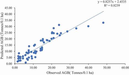
Figure 5. Predicted AGB density map of the study area.

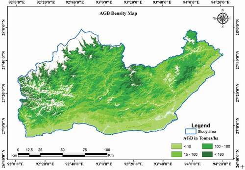
Table 5. AIC for the developed regression analysis of AGB with variables.

Variables	NDVI	SAVI	ARVI	EVI	LST	SM	IM
AIC	219.41	217.74	212.07	219.45	218.51	216.22	176.13
BIC	221.52	219.86	214.19	221.56	220.62	218.33	184.58

IM = integrated Model

4. Discussion

The current study focused on an integrated approach that used freely available optical satellite data-derived SVs, LST, S_m, field inventory measurements, and an empirical modelling approach to predict the spatial AGB of the study region. Although the satellite data-based variables have a significant contribution to the carbon stock modelling process, however, there were certain factors which influenced the satellite data and the data acquisition process that further influence the carbon stock modelling. The study region have very complex landform types ranging from flat to undulating terrain, as well as different land use sectors ranging from grassland to different forest density class, and there surface reflectance is extremely complex, limiting the predictive model’s competence. Further, the use of multi-date satellite data due to unavailability of cloud free satellite data and have different sun and sensor arrangement at the time data acquisition process also doubling the effect on capability of carbon stock process. The variables selection and their characteristics were crucial in AGB predictive model and accuracy of the predictive model is solely dependent on the inherent characteristics of selected variables. Presently, the available variables for the AGB predictive models includes terrain factor, environmental factors, textural feature and SVs (Lu et al., 2014; Zarco-Tejada et al., 2018). The spectral variables include vegetation indices, which were most preferred variables for AGB modelling. The incorporation texture along with terrain factors for some specific area significantly enhances the accuracy of the AGB model (Gleason & Im, 2011). Further, the different forest cover type has different LST performance, which influences the vegetation growth (Neinavaz et al., 2019).

The present predictive model used the Landsat OLI data derived SVs, LST, and S_m. Among the used SVs, although the NDVI was the most preferred VI in the present study, however, it showed a comparably lower correlation with the field-based AGB, this might be attributed due to the high saturation problem at high AGB stock areas. The same was reported that the saturation was caused due to high reflectance in NIR in comparison to low reflectance in red band, which could result inferior correlation (Askar et al., 2018). Due to the correction in soil brightness factor, the SAVI minimized the soil reflectance over the canopy reflectance properties, and have showed better performance than the NDVI (Huete et al., 1994; Vidhya et al., 2014). Among the selected SVs, the ARVI minimizes the atmospheric aerosols brightness effect of the earth’s surface feature reflectance properties, and hence have the better correlation (R² = 0.64) with the AGB, than the other SVs (Huete & Liu, 1994; Tanré et al., 1990).

The multi-linear regression approach using the SVs, LST and S_m was applied to AGB model and AGB estimation. The incorporation of the LST and S_m in the predictive model showed the improvement in accuracy, which was further evaluated by the decrease in RMSE (Table 4). The performance of the predictive model further assessed through the AIC value obtained from the statistical analysis of selected variables (Table 4). The AIC (Bordoloi et al., 2022) and BIC (Yu et al., 2019) index showed the better competence in linear indices for the predictive AGB model. Hence, both AIC and BIC tested in the present study and observed lower AIC and BIC value for the IM among the individual model using each variable, can be compared with AIC and BIC value of above study. Hence, from the present analysis, it was observed that using satellite data derived VIs as predictor variable quite helpful in AGB prediction due to their sensitivity of minimizing the terrain, atmosphere, and soil brightness effect on surface reflectance properties (Lu et al., 2014). The RMSE thus obtained using Landsat data from the study can be compared with the value reported by (B. Li et al., 2018).

The mean AGB predicted from the present study was 131.04 t ha⁻¹ which can be compared with the findings of studies that used Landsat OLI for the different region (B. Li et al., 2018; López-Serrano et al., 2020; Suhardiman et al., 2018). The mean AGB can also be compared with mean AGB (92 t ha⁻¹) reported by Haripriya (2002) for the Indian forest. Y. Li et al. (2020) reported that the mean AGB in range of 16.76 to 173.72 t ha⁻¹ for the subtropical forest of Chenzhou City of China. The mean AGB predicted for plantation was 88.47 t ha⁻¹. Devagiri et al. (2013) estimated comparably slightly higher. The mean predicted AGB for the tropical plantations (185.95 t ha⁻¹) showed higher mean AGB (118.19 t ha⁻¹) for teak plantation of Karnataka. Similarly, Sahu et al. (2016) had also reported higher AGB of 181.2 t ha⁻¹ for Mangrove plantation of Odisha.

5. Pros and cons

The incorporation of numerous variables and factors in predictive AGB model may lead to uncertainty and caused estimation error. The selected variables significantly influence the estimation model performances (S. Chen et al., 2019). Beside this, the sensor type, approach of sampling strategy and estimation model (Lu et al., 2014) were also major factor for AGB estimation model. Presently, optical data like Sntinel-2, Landsat-8, and SPOT images have major contribution in large scale AGB estimation (Y. Chen et al., 2019; Lu et al., 2014; Zhou et al., 2020). Among all the optical data, Landsat series have been providing data with medium resolution with great revisit time. The Landsat-8 onboard TIRS sensor effectively used in LST retrieval, which significantly enhances the accuracy of AGB model (Gleason & Im, 2011; Kim et al., 2014). However, optical data fails to provide the canopy information and have higher saturation mainly in area having dense forest cover (Zhao et al., 2016; Zhu & Liu, 2015). The researcher like Tian et al. (2019) and Cao et al. (2018) have successfully used Airborne laser scanning (ALS) and terrestrial laser scanning (TLS) in small scale AGB estimation with excellent accuracy. However, the inherent character of the sensors and resolution makes it, difficult in large scale study.

The linear approaches are quite simple and can depict the relationships smoothly among the selected variables; however, it fails in reflecting the relationships between the AGB and selected variables under complex forest conditions (S. Chen et al., 2019). Further, the elimination of collinearity among the variables are prerequisite to ensure the significance and interpretability of variables, as these may lead to deletion of highly related variables with AGB (S. Chen et al., 2019).

6. Conclusion

To study the regional and global carbon cycle monitoring, forest dynamic management, the mapping of AGB spatial distribution among the different forest types are crucial. The present study mainly emphasized the utilization of integrated approach which combined the non-destructive, satellite data derived SVs, LST, S_m and empirical modelling algorithms to predict the spatial distribution of AGB of the Study area. From the study, it was evident that the using of optical satellite derived SVs, LST and S_m as dependant variables smoothen the AGB prediction process of the study area. Further, the use of linear method to select the optimum variables may render the accuracy of the AGB model. Hence, non-linear method may be used to get better performance. Besides, optical data, the use SAR, LiDAR satellite data will have an advantage in determining forest structural parameter than the optical data, and hence have the better capability to predict the AGB. The use of deep learning techniques which includes artificial neural network, fuzzy logic, and cellular automata, also has better prospects to model the AGB. The proposed integrated approach will have significant role for the planner and decision makers to achieve the carbon stock management along with their climate change mitigation at the regional level as well as national and global level.

Disclosure statement

No potential conflict of interest was reported by the author(s).

References

- Achat, D. L., Fortin, M., Landmann, G., Ringeval, B., & Augusto, L. (2015). Forest soil carbon is threatened by intensive biomass harvesting. Scientific Reports, 5(1), 15991. https://doi.org/10.1038/srep15991
- Aho, K., DErryberry, D., & Peterson, T. (2014). Model selection for ecologist: The worldviews of AIC and BIC. Ecology, 95(3), 631–636. https://doi.org/10.1890/13-1452.1
- Akaike, H. (1974). A new look at the statistical model identification. EEE Transactions on Automatic Control, 19(6), 716–723. https://doi.org/10.1109/TAC.1974.1100705
- Armenteras, D., Murcia, U., Gonza´ Lez, T. M., Baro´ N, O. J., & Arias, J. E. (2019). Scenarios of land use and land cover change for NW Amazonia: Impact on forest intactness. Global Ecology and Conservation, 17, e00567. https://doi.org/10.1016/j.gecco.2019.e00567
- Askar, N., Phairuang, N., Wicaksono, W., Sayektiningsih, T., & Sayektiningsih, T. (2018). Estimating Aboveground biomass on private forest using sentinel-2 imagery”. Journal of Sensors, 6745629, 1–11. https://doi.org/10.1155/2018/6745629
- Avdan, U., & Jovanovska, G. (2016). Algorithm for automated mapping of land surface temperature using LANDSAT 8 satellite data. Journal of Sensors, 2016, 1480307. https://doi.org/10.1155/2016/1480307
- Bordoloi, R., Das, B., Tripathi, O. P., Sahoo, U. K., Nath, A. J., Deb, S., Das, D. J., Gupta, A., Devi, N. B., Charturvedi, S. S., Tiwari, B. K., Paul, A., & Tajo, L. (2022). Satellite based integrated approaches to modelling spatial carbon stock and carbon sequestration potential of different land uses of Northeast India. Environmental and Sustainability Indicators, 13, 100166. https://doi.org/10.1016/j.indic.2021.100166
- Brown, S., & Lugo, A. E. (1992). Aboveground biomass estimates for tropical moist forests of the Brazilian Amazon. Interciencia. Caracas, 17(1), 8–18. http://philip.inpa.gov.br/publ_livres/Other%20side-outro%20lado/Brown%20%26%20Lugo%20biomass/Brown%20and%20Lugo%201992-Aboveground%20biomass%20estimates.pdf
- Calvao, T., & Palmeirim, J. M. (2004). Mapping mediterranean scrub with satellite imagery: Biomass estimation and spectral behaviour. International Journal of Remote Sensing, 25(16), 3113–3126. https://doi.org/10.1080/01431160310001654978
- Cao, L., Pan, J., Li, R., Li, J., & Li, Z. (2018). Integrating airborne LiDAR and optical data to estimate forest aboveground biomass in arid and semi-arid regions of China. Remote Sensing, 10(4), 532. https://doi.org/10.3390/rs10040532
- Chave, J., Andalo, C., Brown, S., Cairns, M. A., Chambers, J. Q., Eamus, D., Foster, H., Fromard, F., Higuchi, N., Kira, T., Lescure, J. P., Nelson, B. W., Ogawa, H., Puig, H., Riera, B., & Yamakura, T. (2005). Tree allometry and improved estimation of carbon stocks and balance in tropical forests. Oecologia, 145(1), 87–99. https://doi.org/10.1007/s00442-005-0100-x
- Chave, J., Réjou‐Méchain, M., Búrquez, A., Chidumayo, E., Colgan, M. S., Delitti, W. B., Vieilledent, G., Eid, T., Fearnside, P. M., Goodman, R. C., Henry, M., Martínez-Yrízar, A., Mugasha, W. A., Muller-Landau, H. C., Mencuccini, M., Nelson, B. W., Ngomanda, A., Nogueira, E. M., Ortiz-Malavassi, E., … Vieilledent, G. (2014). Improved allometric models to estimate the aboveground biomass of tropical trees. Global Change Biology, 20(10), 3177–3190. https://doi.org/10.1111/gcb.12629
- Chen, S., Feng, Z., Chen, P., Ullah Khan, T., & Lian, Y. (2019). Non destructive estimation of the above-ground biomass of multiple tree species in boreal forests of China using terrestrial laser scanning. Forests, 10(11), 936. https://doi.org/10.3390/f10110936
- Chen, Y., Li, L., Lu, D., & Li, D. (2019). Exploring bamboo forest aboveground biomass estimation using Sentinel-2 data. Remote Sensing , 11(1), 7. https://doi.org/10.3390/rs11010007
- Chen, J., Wang, C., Jiang, H., Mao, L., & Yu, Z. (2011). Estimating soil moisture using Temperature/Vegetation Dryness Index (TVDI) in the Huang-Huai-Hai (HHH) plain. International Journal of Remote Sensing, 32(4), 1165–1177. https://doi.org/10.1080/01431160903527421
- Ciais, P., Sabine, C., Bala, G., Bopp, L., Brovkin, V., Canadell, J., Chhabra, A., DeFries, R., Galloway, J., Heimann, M., Jones, C., Quéré, Le. C., Myneni, R.B., Piao, S., & Thornton, P. (2014). Carbon and other biogeochemical cycles. In T. F. Stocker, D. Qin, G. Plattner, K. M. Tignor, S. K. Allen, J. Boschung, A. Nauels, Y. Xia, V. Bex, & P. M. Midgley (Eds.), Climate change 2013: The physical science basis. Contribution of working group I to the fifth assessment report of the intergovernmental panel on climate change (pp. 465–570). United Kingdom and New York, NY, USA: Cambridge University Press
- Civco, D. L. (1989). Topographic normalization of Landsat Thematic Mapper digital imagery. Photogrammetry and Engineering Remote Sensing, 55(9), 1303–1309.
- Debortoli, N. S., Dubreuil, V., Hirota, M., Filho, S. R., Lindoso, D., & Nabucet, J. (2017). Detecting deforestation impacts in Southern Amazonia rainfall using rain gauges. International Journal of Climatology, 37(6), 2889–2900. https://doi.org/10.1002/joc.4886
- Deka, J., Yumnam, J., Mahanta, P., & Tripathi, O. P. (2015). Improvement in estimation of above ground biomass of albizia lebbeck using fraction reflectance of landsat TM data. International Journal of Plant and Environment, 1(1). https://doi.org/10.18811/ijpen.v1i1.7118
- Devagiri, G. M., Money, S., Singh, S., Dadhawal, V. K., Patil, P., Khaple, A., Devakumar, A. S., & Hubballi, S. (2013). Assessment of above ground biomass and carbon pool in different vegetation types of south western part of Karnataka, India using spectral modeling. Tropical Ecology, 54(2), 149–165.
- Dong, L., Du, H., Han, N., Li, X., Zhu, D., Mao, F., Zhang, M., Zheng, J., Liu, H., Huang, Z., & He, S. (2020). Application of convolutional neural network on lei bamboo above-ground-biomass (AGB) estimation using Worldview-2. Remote Sensing, 12(6), 958. https://doi.org/10.3390/rs12060958
- Du, L., Zhou, T., Zou, Z., Zhao, X., Huang, K., & Wu, H. (2014). Mapping forest biomass using remote sensing and national forest inventory in China. Forests, 5(6), 1267–1283. https://doi.org/10.3390/f5061267
- Eckert, S. (2012). Improved forest biomass and carbon estimations using texture measures from worldView-2 satellite data. Remote Sensing, 4(4), 810–829. https://doi.org/10.3390/rs4040810
- FSI. (1996). Volume equations for forests of India, Nepal and Bhutan. forest survey of india, ministry of environment and forests. Government of India.
- Gleason, C. J., & Im, J. (2011). A review of remote sensing of forest biomass and biofuel: Options for small-area applications. GIScience & Remote Sensing, 48(2), 141–170. https://doi.org/10.2747/1548-1603.48.2.141
- Goetz, S. J., & Dubayah, R. O. (2011). Advances in remote sensing technology and implications for measuring and monitoring forest carbon stocks and change. Carbon Management, 2(3), 231–244. https://doi.org/10.4155/cmt.11.18
- GOFC-GOLD., 2014. A sourcebook of methods and procedures for monitoring and reporting anthropogenic greenhouse gas emissions and removals associated with deforestation, gains and losses of carbon stocks in forests remaining forests, and forestation. GOFC-GOLD Report version COP18-1The
- Gunawardena, A. R., Nissanka, S. P., Dayawansa, N. D. K., & Fernando, T. T. (2015). Estimation of above ground biomass in Horton plains national park, Sri Lanka using Optical, thermal and RADAR remote sensing data. Tropical Agricultural Research, 26(4), 608–623. https://doi.org/10.4038/tar.v26i4.8123
- Günlü, A., Ercanli, İ., Ba, E. Z., & Çak, G. (2014). Estimating aboveground biomass using Landsat TM imagery : A case study of Anatolian crimean pine forests in Turkey. Annals of Forest Research, 57(2), 289–298. https://doi.org/10.15287/afr.2014.278
- Haripriya, G. S. (2002). Biomass carbon of truncated diameter classes in Indian forests. Forest Ecology and Management, 168(1–3), 1–13. https://doi.org/10.1016/S0378-1127(01)00729-0
- Holland, P. G., & Steyn, D. G. (1975). Vegetational responses to latitudinal variations in slope angle and aspect. Journal of Biogeography, 2(3), 179–183. https://doi.org/10.2307/3037989
- Huete, A. R. (1988). A soil-adjusted vegetation index (SAVI). Remote Sensing of Environment, 25(3), 295–309. https://doi.org/10.1016/0034-4257(88)90106-X
- Huete, A., Justice, C., & Liu, H. (1994). Development of vegetation and soil indices for MODIS-EOS. Remote Sensing of Environment, 49(3), 224–234. https://doi.org/10.1016/0034-4257(94)90018-3
- Huete, A. R., & Liu, H. Q. (1994). An error and sensitivity analysis of the atmospheric-and soil-correcting variants of the NDVI for the MODIS-EOS. IEEE Transactions on Geoscience and Remote Sensing, 32(4), 897–905. https://doi.org/10.1109/36.298018
- IPCC. (2006). Forest Land. IPCC guidelines for national greenhouse gas inventories. In H. S. Eggleston, L. Buendia, K. Miwa, T. Ngara, & K. Tanabe (Eds.), Prepared by the national greenhouse gas inventories programme. Japan: IGES.
- Jiang, F., Kutia, M., Ma, K., Chen, S., Long, J., & Sun, H. (2021). Estimating the aboveground biomass of coniferous forest in Northeast China using spectral variables, land surface temperature and Soil moisture. Science of the Total Environment, 785, 147335. https://doi.org/10.1016/j.scitotenv.2021.147335
- Kashung, Y., Das, B., Deka, S., Bordoloi, R., Paul, A., & Tripathi, O. P. (2018). Geospatial technology based diversity and above ground biomass assessment of woody species of West Kameng district of Arunachal Pradesh. Forest Science and Technology, 14(2), 84–90. https://doi.org/10.1080/21580103.2018.1452797
- Kaufman, Y. J., & Tanre, D. (1992). Atmospherically resistant vegetation index (ARVI) for EOS-MODIS. IEEE Transactions on Geoscience and Remote Sensing, 30(2), 261–270. https://doi.org/10.1109/36.134076
- Kim, D.-H., Sexton, J. O., Noojipady, P., Huang, C., Anand, A., Channan, S., Feng, M., & Townshed, J. (2014). Global, Landsat-based forest-cover change from 1990 to 2000. Remote Sensing of Environment, 155, 178–193. https://doi.org/10.1016/j.rse.2014.08.017
- Lal, R. (2005). Forest soils and carbon sequestration. Forest Ecology and Management, 220(1–3), 242–258. https://doi.org/10.1016/j.foreco.2005.08.015
- Lawrence, D., & Vandecar, K. (2015). Effects of tropical deforestation on climate and agriculture. Nature Climate Change, 5(1), 27–36. https://doi.org/10.1038/nclimate2430
- Le Quéré, C., Andrew, R. M., Canadell, J. G., Sitch, S., Korsbakken, J. I., Peters, G. P., Manning, A. C., Boden, T. A., Tans, P. P., Houghton, R. A., Keeling, R. F., Alin, S., Andrews, O. D., Anthoni, P., Barbero, L., Bopp, L., Chevallier, F., Chini, L. P., and Zaehle, S. (2016). Global carbon budget 2016. Earth System Science Data, 8(2), 605–649. https://doi.org/10.5194/essd-8-605-2016
- Le Quéré, C., Andrew, R. M., Friedlingstein, P., Sitch, S., Hauck, J., Pongratz, J., Pickers, P. A., Korsbakken, J. I., Peters, G. P., Canadell, J. G., Arneth, A., Arora, V. K., Barbero, L., Bastos, A., Bopp, L., Chevallier, F., Chini, L. P., Ciais, P., Doney, S. C., … Zheng, B. (2018). Global carbon budget 2018. Earth System Science Data, 10(4), 2141–2194. https://doi.org/10.5194/essd-10-2141-2018
- Li, C., Li, Y., & Li, M. (2019). Improving forest aboveground biomass (AGB) estimation by incorporating crown density and using landsat 8 OLI images of a subtropical forest in western hunan in central China. Forests, 10(2), 104. https://doi.org/10.3390/f10020104
- Li, Y., Li, C., Li, C., Liu, Z., & Elbe-Bürger, A. (2020). Forest aboveground biomass estimation using Landsat 8 and Sentinel-1A data with machine learning algorithms. Scientific Reports, 10(1), 9952. https://doi.org/10.1038/s41598-019-56847-4
- Liu, H. Q., & Huete, A. (1995). A feedback based modification of the NDVI to minimize canopy background and atmospheric noise. IEEE Transactions on Geoscience and Remote Sensing, 33(2), 457–465. https://doi.org/10.1109/TGRS.1995.8746027
- Li, B., Wang, W., Bai, L., Chen, N., & Wang, W. (2018). Estimation of aboveground vegetation biomass based on Landsat-8 OLI satellite images in the Guanzhong Basin, China. International Journal of Remote Sensing, 40(10), 3927–3947. https://doi.org/10.1080/01431161.2018.1553323
- López-Serrano, P. M., Cárdenas Domínguez, J. L., Corral-Rivas, J. J., Jiménez, E., López-Sánchez, C. A., & Vega-Nieva, D. J. (2020). Modeling of Aboveground biomass with LANDSAT 8 OLI and machine learning in temperate forests. Forests, 11(1), 11. https://doi.org/10.3390/f11010011
- Lu, D. (2006). The potential and challenge of remote sensing‐based biomass estimation. International Journal of Remote Sensing, 27(7), 1297–1328. https://doi.org/10.1080/01431160500486732
- Lu, D., Chen, Q., Wang, G., Liu, L., Li, G., and Moran, E. (2014). A survey of remote sensing–based aboveground biomass estimation methods in forest ecosystems. International Journal of Digital Earth, 9(1), 63–105. https://doi.org/10.1080/17538947.2014.990526
- MacDicken, K. G. (1997). A guide to monitoring carbon storage in forestry and agroforestry projects. Winrock International Institute for Agricultural Development, Forest Carbon Monitoring Programme.
- Måren, I. E., Karki, S., Prajapati, C., Yadav, R. K., & Shrestha, B. B. (2015). Facing north or south: Does slope aspect impact forest stand characteristics and soil properties in a semiarid trans-Himalayan valley? Journal of Arid Environments, 121, 112–123. https://doi.org/10.1016/j.jaridenv.2015.06.004
- McGarvey, J. C., Thompson, J. R., Epstein, H. E., & Shugart, H. (2015). Carbon storage in old-growth forests of the Mid-Atlantic: Toward better understanding the eastern forest carbon sink. Ecology, 96(2), 311–317. https://doi.org/10.1890/14-1154.1
- Motlagh, M. G., Kafaky, S. B., Mataji, A., & Akhavan, R. (2018). Estimating and mapping forest biomass using regression models and Spot-6 images (case study: Hyrcanian forests of north of Iran). Environmental Monitoring and Assessment, 190, 352. https://doi.org/10.1007/s10661-018-6725-0
- Nath, A. J., Tiwari, B. K., Sileshi, G. W., Sahoo, U. K., Brahma, B., Deb, S., Devi, N., Das, A., Reang, D., Chaturvedi, S., Tripathi, O., Das, D., & Gupta, A. (2019). Allometric models for estimation of forest biomass in North East India. Forests, 10(2), 103. https://doi.org/10.3390/f10020103
- Neinavaz, E., Darvishzadeh, R., Skidmore, A. K., & Abdullah, H. (2019). Integration of Landsat-8 thermal and visible-short wave infrared data for improving prediction accuracy of forest leaf area index. Remote Sensing, 11(4), 390. https://doi.org/10.3390/rs11040390
- Norovsuren, B., Tseveen, B., Batomunkuev, V., & Renchin, T. (2020). Estimation for forest biomass and coverage using Satellite data in small scale area, Mongolia. In IOP Conference Series: Earth and Environmental Science, 320( 1), 012019.
- Pachauri, R. K., & Reisinger, A. (2007). Contribution of working groups I, II and III to the fourth assessment report of the intergovernmental panel on climate change IPCC.
- Pandey, P. C., Koutsias, N., Petropoulos, G. P., Srivastava, P. K., & Ben Dor, E. (2019). Land use/land cover in view of earth observation: Data sources, input dimensions, and classifiers—a review of the state of the art. Geocarto International, 36(9), 957–988. https://doi.org/10.1080/10106049.2019.1629647
- Pearson, T. R., Brown, S., Murray, L., & Sidman, G. (2017). Greenhouse gas emissions from tropical forest degradation: An underestimated source. Carbon Balance Management, 12(1), 3. https://doi.org/10.1186/s13021-017-0072-2
- Powell, S. L., Cohen, W. B., Healey, S. P., Kennedy, R. E., Moisen, G. G., Pierce, K. B., & Ohmann, J. L. (2010). Quantification of live aboveground forest biomass dynamics with Landsat time-series and field inventory data: A comparison of empirical modeling approaches. Remote Sensing of Environment, 114(5), 1053–1068. https://doi.org/10.1016/j.rse.2009.12.018
- Przeździecki, K., Zawadzki, J., Cieszewski, C., & Bettinger, P. (2017). Estimation of soil moisture across broad landscapes of Georgia and South Carolina using the triangle method applied to MODIS satellite imagery. Silva Fennica, 51(4), 1683. https://doi.org/10.14214/sf.1683
- Qureshi, A., Hussain, S. A., Hussain, S. A., & Hussain, S. A. (2012). A review of protocols used for assessment of carbon stock in forested landscapes. Environmental Science & Policy, 16, 81–89. https://doi.org/10.1016/j.envsci.2011.11.001
- Ramachandra, T. V., & Bharath, S. (2019). Global warming mitigation through carbon sequestrations in the Central Western Ghats. Remote Sensing in Earth Systems Sciences, 2(1), 39–63. https://doi.org/10.1007/s41976-019-0010-z
- Ramachandra, T. V., & Bharath, S. (2020). Carbon sequestration potential of the forest ecosystems in the Western Ghats, a global biodiversity hotspot. Natural Resources Research, 29(4), 2753–2771. https://doi.org/10.1007/s11053-019-09588-0
- Ramachandra, T. V., Bharath, S., & Gupta, N. (2018). Modelling landscape dynamics with LST in protected areas of Western Ghats, Karnataka. Journal of Environmental Management, 206, 1253–1262. https://doi.org/10.1016/j.jenvman.2017.08.001
- Ramankutty, N., Gibbs, H. K., Achard, F., DeFries, R., Foley, J. A., & Houghton, R. A. (2007). Challenges to estimating carbon emissions from tropical deforestation. Global Change Biology, 13(1), 51–66. https://doi.org/10.1111/j.1365-2486.2006.01272.x
- Ravindranath, N. H., Chaturvedi, R. K., & Murthy, I. K. (2008). Forest conservation, afforestation and reforestation in India: Implications for forest carbon stocks. Current Science, 95(2), 216–222. http://www.ias.ac.in/currsci/jul252008/216.pdf
- Ren, H., & Zhou, G. (2014). Determination of green aboveground biomass in desert steppe using litter-soil-adjusted vegetation index. European Journal of Remote Sensing, 47(1), 611–625. https://doi.org/10.5721/EuJRS20144734
- Rouse, J. W., Haas, R. H., Hell, J. A., Deering, D. W., & Harlan, J. C. (1974). Monitoring the vernal advancement of retrogradation (greenwave effect) of natural vegetation. In M. D. Greenbelt (Ed.), NASA/GSFC, Type III, Final Report (pp. 371).
- Sahu, S. C., Kumar, M., & Ravindranath, N. H. (2016). Carbon stocks in natural and planted mangrove forests of Mahanadi Mangrove Wetland, East Coast of India. Current Science, 110(12), 2253–2260. https://doi.org/10.18520/cs/v110/i12/2253-2260
- Sandholt, I., Rasmussen, K., & Andersen, J. (2002). A simple interpretation of the surface temperature/vegetation index space for assessment of surface moisture status. Remote Sensing of Environment, 79(2–3), 213–224. https://doi.org/10.1016/S0034-4257(01)00274-7
- Santos, J. R., Freitas, C. C., Araujo, L. S., Dutra, L. V., Mura, J. C., Gama, F. F., Soler, S. S., & Sant'Anna, S. J. (2003). Airborne P-band SAR applied to the aboveground biomass studies in the Brazilian tropical rainforest. Remote Sensing of Environment, 87(4), 482–493. https://doi.org/10.1016/j.rse.2002.12.001
- Sarker, L. R., & Nichol, J. E. (2011). Improved forest biomass estimates using ALOS AVNIR-2 texture indices. Remote Sensing of Environment, 115(4), 968–977. https://doi.org/10.1016/j.rse.2010.11.010
- Sharma, C., Gairola, S., Ghildiyal, S. K., & Suyal, S. (2010). Physical properties of soils in relation to forest composition in moist temperate valley slopes of the Central Western Himalaya. Journal of Forest Science, 26, 117–129. http://ocean.kisti.re.kr/downfile/volume/ifsknu/SRGHBV/2010/v26n2/SRGHBV_2010_v26n2_117.pdf
- Shen, G., Wang, Z., Liu, C., & Han, Y. (2020). Mapping aboveground biomass and carbon in Shanghai’s urban forest using Landsat ETM+ and inventory data. Urban Forestry & Urban Greening, 51, 126655. https://doi.org/10.1016/j.ufug.2020.126655
- Sobrino, J. A., Jim´enez-Mu˜noz, J. C., & Paolini, L. (2004). Land surface temperature retrieval from LANDSAT TM5. Remote Sensing of Environment, 90(4), 434–440. https://doi.org/10.1016/j.rse.2004.02.003
- Stovall, A. E., Vorster, A. G., Anderson, R. S., Evangelista, P. H., & Shugart, H. H. (2017). Non-destructive aboveground biomass estimation of coniferous trees using terrestrial LiDAR. Remote Sensing of Environment, 200, 31–42. https://doi.org/10.1016/j.rse.2017.08.013
- Suhardiman, A., Tampubolon, B. A., & Sumaryono, M. (2018). Examining spectral properties of Landsat 8 OLI for predicting above-ground carbon of Labanan Forest, Berau. IOP Conference Series: Earth and Environmental Science. 144, 012064.
- Tang, X., Fehrmann, L., Guan, F., Forrester, D., Guisasola, R., & Kleinn, C. (2016). Inventory based estimation of forest biomass in Shitai County, China: A comparison of five methods. Annals of Forest Research, 59(1), 269–280. https://doi.org/10.15287/afr.2016.574
- Tanré, D., Deroo, C., Duhaut, P., Herman, M., Morcrette, J. J., Perbos, J., & Deschamps, P. Y. (1990). Technical note Description of a computer code to simulate the satellite signal in the solar spectrum: The 5S code. International Journal of Remote Sensing, 11(4), 659–668. https://doi.org/10.1080/01431169008955048
- Thenkabail, P. S., Stucky, N., Griscom, B. W., Ashton, M. S., Diels, J., Van der Meer, B., & Enclona, E. (2004). Biomass estimations and carbon stock calculations in the oil palm plantations of African derived savannas using IKONOS data. International Journal of Remote Sensing, 25(23), 5447–5472. https://doi.org/10.1080/01431160412331291279
- Tian, J., Dai, T., Li, H., Liao, C., Teng, W., Hu, Q., Ma, W., & Xu, Y. (2019). A novel tree height extraction approach for individual trees by combining TLS and UAV image-based point cloud integration. Forests, 10(7), 537. https://doi.org/10.3390/f10070537
- UNFCCC. 2009. Reducing emissions from deforestation in developing countries: Approaches to stimulate action. FCCC/SBSTA/2009/19/Add.1. FCCC/SBSTA/2009/19/Add.1.
- UN-REDD., 2011. The UN-REDD programme strategy 2011-2015. https://www.iisd.org/pdf/2011/redd_programme_strategy_2011_2015_en.pdf
- Urbazaev, M., Thiel, C., Migliavacca, M., Reichstein, M., Rodriguez-Veiga, P., & Schmullius, C. (2016). Improved multi-sensor satellite-based aboveground biomass estimation by selecting temporally stable forest inventory plots using NDVI time series. Forests, 7(8), 169. https://doi.org/10.3390/f7080169
- Vidhya, R., Vijayasekaran, D., Farook, M. A., Jai, S., Rohini, M., & Sinduja, A. (2014). Improved classification of mangroves health status using hyperspectral remote sensing data. The International Archives of Photogrammetry, Remote Sensing and Spatial Information Sciences, 40(8), 667. https://doi.org/10.5194/isprsarchives-XL-8-667-2014
- Wu, C., Shen, H., Shen, A., Deng, J., Gan, M., Zhu, J., Xu, H., & Wang, K. (2016). Comparison of machine-learning methods for above-ground biomass estimation based on Landsat imagery. Journal of Applied Remote Sensing, 10(3), 035010. https://doi.org/10.1117/1.JRS.10.035010
- Yadav, A. S., & Gupta, S. K. (2006). Effect of micro-environment and human disturbance on the diversity of woody species in the Sariska Tiger Project in India. Forest Ecology and Management, 225, 178–189. https://doi.org/10.1016/j.foreco.2005.12.058
- Yu, X., Ge, H., Lu, D., Zhang, M., Lai, Z., & Yao, R. (2019). Comparative study on variable selection approaches in establishment of remote sensing model for forest biomass estimation. Remote Sensing, 11(12), 1437. https://doi.org/10.3390/rs11121437
- Zanter, K. (2019). Landsat 8 (L8) data users Handbook; LSDS-1574 v.5.0; Department of the Interior U.S. geological survey. EROS.
- Zarco-Tejada, P. J., Hornero, A., Hernández-Clemente, R., & Beck, P. S. A. (2018). Understanding the temporal dimension of the red-edge spectral region for forest decline detection using high-resolution hyperspectral and Sentinel-2a imagery. ISPRS Journal of Photogrammetry and Remote Sensing, 137, 134–148. https://doi.org/10.1016/j.isprsjprs.2018.01.017
- Zhao, P., Lu, D., Wang, G., Wu, C., Huang, Y., & Yu, S. (2016). Examining spectral reflectance saturation in Landsat imagery and corresponding solutions to improve forest aboveground biomass estimation. Remote Sensing, 8(6), 469. https://doi.org/10.3390/rs8060469
- Zheng, D., Rademacher, J., Chen, J., Crow, T., Bresee, M., Le Moine, J., & Ryu, S. R. (2004). Estimating aboveground biomass using Landsat 7 ETM+ data across a managed landscape in northern Wisconsin, USA. Remote Sensing of Environment, 93(3), 402–411. https://doi.org/10.1016/j.rse.2004.08.008
- Zhou, J., Zhou, Z., Zhao, Q., Han, Z., Wang, P., Xu, J., & Dian, Y. (2020). Evaluation of different algorithms for estimating the growing stock volume of Pinus massoniana plantations using spectral and spatial information from a SPOT6 image. Forests, 11(5), 540. https://doi.org/10.3390/f11050540
- Zhu, X., & Liu, D. (2015). Improving forest aboveground biomass estimation using seasonal Landsat NDVI time-series. ISPRS Journal of Photogrammetry and Remote Sensing, 102, 222–231. https://doi.org/10.1016/j.isprsjprs.2014.08.014