Soil and water relations in mangrove ecosystems in Guyana

ABSTRACT

In mangrove forests, one of the most noticeable characteristics is the unique interplay between soil and water, which facilitates the movement of nutrients and sediments throughout their ecosystems. In this study, comparisons were made between the physicochemical characteristics of soil (pH, EA, OC, EC, N, P, K, Mg, Ca, S, Fe, Zn, Cu, and Mn) and water (pH, temperature, and electrical conductivity) found in natural, degraded, and restored mangrove ecosystems along the coastline of Guyana. Sampling was done using a Random Block Design (RBD) in six study sites for six months. This study revealed that there were no significant variations in most of the physicochemical parameters found in soil and water within ecosystem type or season. However, notable differences were seen in the pH of water (6.45–7.88), as well as Fe (0.60–21.62 ppm, p < 0.05) and Mg (610–3944.67 ppm, p < 0.05) concentrations of soil within the three types of ecosystems. Seasonal differences were also evident in S, N, P, K, and Cu concentrations found within the mangrove soils. In both seasons, positive correlation findings (p < 0.05, R > 0.75) showed higher associations between soil physicochemical properties concerning ecosystem types,  when compared to water parameters.

KEYWORDS:

• Mangroves
• ecosystems
• Guyana
• mangrove sediments

Introduction

Mangroves can be described as coastal marine forests consisting of shrubs, palms, ferns, epiphytes, and trees. Mangrove forests are found at the interface between land and water; therefore, they are found in both the aquatic and terrestrial realms and play crucial roles in both areas (Rog et al., 2016). These forests can withstand harsh environmental stresses and are uniquely adapted to marine and estuarine tidal conditions (Alappatt, 2008; Lewis et al., 2016). Mangroves serve as a connection between freshwater and marine ecosystems, a source of nutrient flux into marine ecosystems, and a sink for contaminants (Maiti & Chowdhury, 2013). The intertidal ecotones of estuaries and open coastlines, as well as the dynamics of shifting water levels, temperatures, erosion, and pioneer habitats, are where mangrove forest ecosystems get their biological significance. Mangrove ecosystems are described as diverse and have been adjusted to the extreme conditions of highly salty, often flooded, soft, anoxic soils (Khairnar et al., 2009). These particular circumstances lead to biodiversity hotspots in a small number of nations (Getzner & Islam, 2020).

Mangroves are known to provide several important ecological goods and services to a number of countries, especially in Guyana. Timber extraction, critical coastal protection, flood management, and the sustainability of fisheries and wildlife in coastal environments are examples of such ecological goods and services (Guyana Forestry Commission, 2017). Mangroves defend Guyana’s fragile coastlines from strong currents by holding the soil together and preventing coastal erosion, which is perhaps their most essential function. During wet periods and stormy conditions, mangroves also protect inland areas and reduce damage (Guyana Forestry Commission, 2011). These unique forests are known to be the home of a diverse range of flora and fauna. Migratory shorebirds, waders, waterfowl, fishes, mammals, crustaceans, and reptiles depend on mangroves for nesting areas during high tides, for protection, and as a food source (Dookram et al., 2017). Furthermore, mangrove trees disintegrate contaminants play an important role in sequestering carbon and provide several products, including charcoal, fodder, honey, tannin, medicine, and thatch (Ackroyd, 2010; Jaikishun et al., 2017).

When mangrove stocks are depleted due to pollution or land removal, society itself becomes detached from the flow of ecosystem services that it provides (Moonsammy, 2021). The degradation of mangrove habitats manifests a decline in biodiversity richness, ecological diversity, and the production of services and items (Friess et al., 2019). Despite their significance, mangroves are being degraded at a rate of 1–2% globally annually, and the loss rate has escalated to 35% over the past 20 years. In general, the main threats to mangrove environments are climate change (sea level rise and changing patterns of precipitation) and human impacts (urban growth, aquaculture, quarrying, and overharvesting of timber, fish, shellfish, and crustaceans(Carugati et al., 2018). Biodiversity decline is frequently correlated with habitat destruction. According to theoretical ecology, ecosystem functionality can be influenced by biodiversity (Cardinale et al., 2006). Although the functionality of maritime ecosystems and biodiversity are frequently correlated, biodiversity loss could reduce the functioning of ecosystems and, as a consequence, the potential of such ecosystems to offer goods and services to humans (Polidoro et al., 2010). This is especially true in tropical mangrove habitats, which support a significant portion of coastal biodiversity and will be affected by factors that have manifested due to climate change (Alongi, 2015). Given their tidal composition, sea-level rise represents the principal concern. Nevertheless, it is also essential to take into account variations in temperature, salinity, and greenhouse gas concentrations. Furthermore, fluctuations in precipitation can also affect the soil-water content and salinity, which can alter mangrove growth and species diversity (Lee et al., 2014). In Guyana, 33, 277 ha of mangroves currently cover coastal regions from Barima–Waini to East Berbice–Corentyne, with the most intact forests residing in Region 1 (Barima–Waini) and the least intact in Region 4 (Demerara-Mahaica) ([EAME] Earth and Marine Environmental Consultants, 2018) (Figure 1). However, Guyana’s coastal belt is frequently exposed to considerable erosion as a result of strong currents. A 238 km-long stonework and earthen barricaded sea defence structure is regularly broken, causing economic damage to crop plants and homes due to encroaching seawater. The entire coast of Guyana was fringed by mangrove vegetation during colonisation. However, anthropogenic impacts have depleted or destroyed the majority of the forested sections (Winterwerp et al., 2013). Natural erosional and accretive periods typical of the Guianas’ coastline (along the Amazon River moving towards the Orinoco River), as well as massive shifts in the mud banks, pose significant threats to Guyana’s mangroves (Ahmad & Lakhan, 2012). The emergence of man-made factors (through extensive coastal development) has encouraged cycles of erosion that have continuously removed sections of the mangrove belt (”NAREI”, 2019). Forest loss is primarily caused by mining, logging, farming, and infrastructure construction. During the period from 1990 to 2016, the national deforestation rate peaked in 2012 (0.079%) before dropping to 0.05% in 2016. Mining accounts for approximately 72% of the land area transformed during this period, with forestry, agriculture, and utilities accounting for the remaining 28% (Guyana Forestry Commission, 2017). Significant habitat loss as a result of land usage for urban development, farming, aquaculture, improved infrastructure, as well as overharvesting of mangroves are all anthropogenic factors currently affecting mangroves in Guyana (”NAREI”, 2019).

Figure 1. Mangrove coverage (ha) along the coastline of Guyana, from regions 1–6 (Source: [EAME] Earth and Marine Environmental Consultants, 2018).

In mangrove ecosystems, there is a close connection between sedimentation and hydrodynamics. That is, soil and water movements are intricately linked and operate in unison. Tidal and wave-induced currents carry sediments to sediment deposits, while complex wave motions, on the other hand, may cause sediments between the roots to be remobilised by the water (Toorman et al., 2018). The morphodynamics of mangroves is defined by dynamic interactions that occur between tidal flows and surfaces covered with vegetation throughout mangrove margins (Spencer & Möller, 2013). These interactions are crucial for coastal protection, mangrove forest regeneration, forestry, conservation, and water pollution control (Risanti & Marfai, 2020; Wang et al., 2010). Srilatha et al. (2013) describe how the physicochemical properties of water play an important role in organism distribution, inclusive of feeding and reproduction. As materials are moved between and within mangrove forests with tidal movements, nutrient transfers involving mangrove ecosystems and coastal waters are regulated by the hydrology of these environments (Hayes et al., 2018). Spatial and temporal variations of water parameters such as pH, electrical conductivity, and temperature profoundly affect the survival, development, and regeneration of mangroves (Kodikara et al., 2017). However, the dynamic characteristics of water are directly influenced by physical, biological, and chemical processes like evaporation, solar radiation, and marine climatic conditions (Ward et al., 2016).

Many recent studies have shown that environmental factors can influence the physicochemical properties of water present in mangrove forests. The growth of mangrove stands is influenced by parameters such as pH, salinity (electrical conductivity), and temperature of the water in mangrove forests, which play a significant role in determining the species diversity and productivity of the mangroves (Cabañas-Mendoza et al., 2020; Peters et al., 2020). Due to variations in precipitation, river flow, evaporative demand, and water usage by rival plants, fluctuations in the pH and salinity of coastal settings are predicted to have a significant impact on species composition and growth (Runting et al., 2016). Additionally, climate change is causing sea levels to rise and promoting extreme precipitation events in some areas, which affects the availability of freshwater in the coastal environment (Swales et al., 2019). Furthermore, climate change affects sea surface density via fluctuations in salinity and temperature. This can affect the buoyancy and dispersal of mangrove propagules, thus limiting the expansion and regeneration of forests along the coastline (Van der Stocken et al., 2022). Strong evaporation (amplified by climate change) results in surface water with high temperature and salinity, which can intensify physical stress in mangrove trees and seedlings due to the increased release of contaminants and antioxidants in the water surrounding them (Aljahdali et al., 2021). The requirement to supply water for an expanding human population and their associated agricultural and economic activities has decreased water movements to the coast since some rivers have been redirected for water storage, which also affects the availability of freshwater in coastal areas (Lovelock et al., 2015; Sippo et al., 2016).

Mangrove soils, on the other hand, can support life since they provide a physical foundation for plant anchorage, stabilisation, nutrient availability, water filtration, waste recycling, and purification (Bomfim et al., 2018). Mangrove soils are usually saline, oxygen-deficient, acidic, and often waterlogged (Dissanayake & Chandrasekara, 2014). A sufficient supply of mineral nutrients is needed by mangroves. These consist of micronutrients like iron, zinc, and manganese as well as macronutrients such as nitrogen, phosphorus, and potassium (Hogarth, 2015). Possible nutrient sources include precipitation, freshwater discharge from river systems or the land, tide-borne soluble or particle-bound nutrients, animal importation, nitrogen fixation by bacteria, and release from organic material due to microbial decomposition (Wang et al., 2021). These sources can be significant or unimportant, depending on the specific situation. Although rainfall’s direct contribution to nutrient input is probably negligible, mangrove regions that receive a lot of rain typically receive a lot of freshwater discharge from rivers. In addition, mangroves may also receive nutrients from regular tidal inundations (Alongi, 2020). Along the Guiana Shield, mangrove soils are created when sediments from erosion along the coastline or on riverbanks, as well as soils removed from elevated areas, are moved through various water sources ([NMMAP] National Mangrove Management Action Plan, 2012). Guyana’s coastal system is marked by heavy mud deposits (from the Amazon) along with huge concentrations of mud within its coastal waters (Winterwerp et al., 2007). In slow-moving “slings,” large amounts of soil (composed mainly of clay and silt) are brought along the coast from Northwest areas. As these three-mile-long mud banks advance along the coastline, an observable trend emerges in which as the crest of the bank moves, mud builds up in one region, following a period of degradation as an accompanying mud trough proceeds. The high banks tend to assist in the growth of mangrove forests, while the troughs appear to promote erosion and degradation ([NMMAP] National Mangrove Management Action Plan, 2012).

The physiographical location of mangroves, in addition to structure (mineralogy, organic content, and metal concentrations) (Krauss et al., 2013; Lunstrum & Chen, 2014), can affect the environmental functions and properties of soil. Soils and vegetation interact strongly in mangrove ecosystems, resulting in the development of the former as well as the characteristics of the plant environment (Perera et al., 2013). The physicochemical soil characteristics affect the development of mangrove plant species, which can compromise their growth and structure (Harahap et al., 2015). Mangrove soil texture, which typically ranges from very loose sand to very heavy clay, is described as a very stable feature that affects soil biophysical properties and is long-term interconnected with soil fertility and quality (Yu et al., 2020). Soil texture, which is linked to soil porosity, controls water-holding capability, diffusion, and water movement, both of which influence the soil’s overall health (Upadhyay and Raghubanshi, 2020). Factors such as topography, climate, hydrodynamic cycles, tidal gradients, and long-term ocean level shifts all influence soil morphological and physicochemical characteristics (Boto, 2018; Lugo & Medina, 2020). These factors can cause variations in soil texture and moisture, pH, salinity, cation exchange capacity (CEC), macronutrients, micronutrients, carbon, and organic matter (OM) concentrations (Hossain & Nuruddin, 2016). Furthermore, mangrove soils may vary in different ecosystems based on some environmental conditions such as nutrient availability, soil particle size, tidal effects, texture, moisture, soil fertility, and the extent of disturbances (either natural or anthropogenic; Dewiyanti et al., 2021). This can subsequently affect the water composition, quality, salinity regime, and pollutant removal capacity of a mangrove ecosystem itself (Risanti & Marfai, 2020). Studies have shown that disturbed areas (indicated by decreased numbers of mangroves) have the smallest OM levels along with low nitrogen (N) and potassium (K) concentration levels, while undisturbed mangrove areas possess rich OM content, maximum N and K concentrations, as well as the lowest calcium carbonate (CaCO3), pH, and salinity levels (Shahid et al., 2014; Alsumaiti & Shahid, 2018).

Mangrove tree assemblages play a key role in coastal carbon sequestration and budgeting, preserving a greater proportion of the total environment’s organic carbon (OC) stocks, especially in their rich soil OC pools (Sasmito et al., 2020). Allochthonous and autochthonous are the two primary sources of carbon in mangrove soils (Sasmito et al., 2015; Stringer et al., 2016). Mangrove soils are frequently flooded, either partially or entirely, and therefore have high OM content, which influences pH as well as other physicochemical parameters such as oxide reduction mechanisms (Cabañas-Mendoza et al., 2020; Naidoo, 2016). The pH of mangrove habitats can be affected by dissolved calcium from shells, and brackish waters can become alkaline as a result of offshore corals. According to Hossain and Nuruddin (2016), mangrove soils can be acidic or basic, with pH usually ranging from 2.87 to 8.22. Active acidity and exchangeable acidity are the two elements of soil acidity. Exchangeable acidity (EA) is described as the number of hydrogen ions on cation exchange sites of clay (which is negatively charged) and organic material concentrations in the soil (Onwuka et al., 2016). The acidity of different soil types varies depending on their composition, rainfall amounts, and natural vegetation. Soil pH, often referred to as the “chief soil variable,” influences several biological, physical, and chemical properties and events that influence the growth and biomass production of plants. Soil acidity is altered through leaching, degradation, crop absorption of basic cations (K⁺, Ca²⁺, Mg²⁺, etc.), plant residue deterioration, and plant root exudates throughout different seasons. Soils with increased CEC and a propensity for significant quantities of EA (such as clays as well as those rich in OM) are well buffered (Spargo et al., 2013).

The ability of mangrove trees to access nutrients is regulated by a complicated system of interacting abiotic and biotic factors, and mangroves tend to opportunistically use these nutrients when they become accessible (Reef et al., 2010). According to Lovelock et al. (2005), mangrove soils have significantly lower nutritional availability, but nutrient content and accessibility vary considerably among mangroves as well as within their habitats. Plants require calcium (Ca), magnesium (Mg), and sulphur (S) to thrive. Ca, Mg, and S concentrations are adequate in soils with fair pH and good levels of organic matter. When calcium and magnesium are added to the soil, they raise the pH, but sulphur from certain sources reduces it (Oldham, 2019). Calcium acts as a counter-cation for both inorganic and organic anions, as well as an intracellular transmitter that regulates response to numerous developmental indicators and environmental conditions (Thor, 2019). Sulphur compounds are also used predominantly by sulphur-reducing bacteria (SRB) as well as sulphur-oxidising bacteria (SOB), both of which are critical in mangrove metabolism (SamKamaleson & Gonsalves, 2019). The sulphate ion, SO4, is the form that plants most often absorb and is easily removed from soils by leaching. Sulphate accumulates in heavier (higher clay content) subsoils as it is leached down into the soil (Oldham, 2019). In addition, magnesium plays an important role in photosynthetic activities, enzyme activation, and ATP formation and usage (Cakmak, 2013), inclusive of vital roles like phloem loading and photoassimilates transport directly to sink organs like shoot tips, roots, and seeds. In general, magnesium uptake in plants is influenced by its concentration, behaviour, and the soil’s ability to replenish it in the soil solution (Yan et al., 2018).

Within the group of macronutrients, nitrogen (N), phosphorus (P), and potassium (K) are the most fundamental nutrients for plant development (White & Brown, 2010). Plants use nitrogen to make amino acids, which are then converted into proteins. It is a part of chlorophyll and plays an important role during photosynthesis (Reef et al., 2010). Furthermore, phosphorus, which is found in the soil as a phosphate ion, aids plant mechanisms such as photosynthesis and energy transfer. It also promotes early root development and growth, which allows plants to mature and reproduce faster (Fageria, 2008). Almahasheer et al. (2016) described nitrogen and phosphorus as two nutrients that are most likely to restrict mangrove development. In mangrove soils, ammonium is the most common source of nitrogen. Tree growth is primarily aided by ammonium uptake in mangrove forests due to anoxic soil conditions (Reef et al., 2010). Potassium (Kalium), absorbed by plants as potassium ion (K⁺), is essential for a wide range of plant functions, which includes the activation of numerous enzyme systems involved in carbohydrate and protein synthesis. Potassium (in adequate concentrations) also decreases respiration, lowers the loss of energy, improves the plant’s water regime, and allows them to become resistant to unfavourable conditions such as saline fluctuations in the environment and drought (Fageria, 2008).

According to Kannappan et al. (2012), metals are absorbed and retained by the soils of mangrove forests from a variety of natural and anthropogenic sources, including freshwater, saltwater, and sewage runoff/leakage. Broadley et al. (2012) suggest that metals may be classified as nutrients, trace metals, or heavy metals depending on their degree of denseness. Heavy metals, when used as micronutrients, provide plants with metabolic requirements. However, their absence can impair the entire enzymatic system and, as a result, the overall function of the plant (Singh et al., 2016). Several studies conducted by Kannappan et al. (2012), Madi et al. (2015), and Thanh-Nho et al. (2019) have debated the dual roles of copper (Cu), iron (Fe), zinc (Zn), and manganese (Mn), which can act as nutrients and/or harmful elements in mangrove habitats. Zinc is an essential part of a variety of processes, including co-factoring enzymes, gene expression, biosynthesis of chlorophyll, auxin production, transduction of signals and defence mechanisms, and is also recognised as an essential component in several dehydrogenases, proteinases, and peptidases (Hacisalihoglu, 2020). Similarly, iron (Fe) is essential in a variety of biochemical and physiological mechanisms in plants because it is a constituent of many important enzymes and is thus necessary for a variety of biological processes (Schmidt et al., 2020). Plants need iron for the production of chlorophyll and protein in their leaves, the maintenance of their chloroplast framework, and root development (Thanh-Nho et al., 2019). However, a deficiency of iron is detrimental to chloroplasts because it affects the water-splitting mechanism of photosystem II (PSII), which is responsible for supplying the electrons needed for photosynthesis (Millaleo et al., 2010). Furthermore, manganese (Mn) is active in protein and enzyme structures that are photosynthetic in nature, making it a significant contributor to a variety of biological processes. Copper is needed for electron transfer in photosystem II, mitochondrial and chloroplast processes, carbohydrate processing, protein synthesis, as well as lignification of cell walls, among other enzyme systems (Thanh-Nho et al., 2019). Clay composition, OM, and reduced conditions are all found to be beneficial factors in mangrove soils’ capacity to sequester metals (Nguyen et al., 2020). Sediments from tidal marshes with high clay and OM content and higher negative redox potential can sequester more heavy metals (Almahasheer et al., 2018). As a result, mangrove habitats are highly efficient in the accumulation of metals, which, when combined with their ability to maintain and immobilise soils, results in soil elevations. This implies that mangroves could play a significant role as metal filters and sinks within coastal communities (Nguyen et al., 2020).

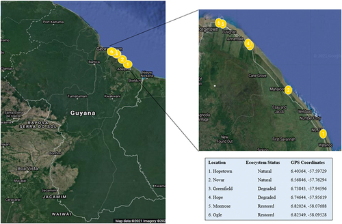
Presently, there exist research gaps in understanding the physicochemical characteristics of soil and water present in Guyana’s mangrove ecosystems due to a lack of published studies on the subject matter. Understanding what is required for the survival, conservation, and restoration of mangrove ecosystems involves knowledge of soil morphology and the physicochemical characteristics of both soil and water (Bomfim et al., 2018). It is also essential to comprehend the extent to which soil and water characteristics in mangrove ecosystems are affected by seasonality. Studies have shown that the physicochemical parameters of soil and water have shown remarkable variations in wet and dry seasons, which can affect the density, litterfall, flowering, fruiting, and nutrient uptake of the plant species found within them (Komiyama et al., 2019; Zhang et al., 2016). In this study, we have monitored the extent of natural and anthropogenic disturbances occurring in six mangrove sites along the coastline of Guyana for six months, which is summarised in Table 1. The types of disturbances recorded during the period of data collection within the mangrove ecosystem sites included natural phenomena such as plant infestation, erosion, storms, tides, and insect infestation. However, anthropogenic activities were more prevalent than natural phenomena, which resulted in disturbances such as bark stripping, grazing, cutting, sand mining, burning, fishing activities, garbage dumping, and infrastructure development. Based on the level of disturbances, mangrove ecosystems were then classified into three types within this study – degraded (D) (ecosystems exposed to a high number of human and natural disturbances/perturbations), natural (N) (ecosystems with little to no disturbances/perturbations–pristine “old growth” trees), and restored (R) (replanted ecosystems now recovering from disturbances/perturbations towards a natural state). In light of the aforementioned, the purpose of this study was to (i) examine the physicochemical characteristics of soil and water found in mangrove ecosystems that are natural, degraded, and restored; and (ii) compare the physicochemical characteristics of soil and water found within these ecosystems in the wet and dry seasons. We believe that the results of this study will guide the scientific community towards a better understanding of soil and water properties present in natural, degraded, and restored mangrove ecosystems in Guyana and the effect of seasonality on such properties.

Table 1. The extent of disturbances occurring within mangrove ecosystems under study.

Location			Ogle	Montrose	Hope	Greenfield	Novar	Hopetown
Ecosystem Type			Restored		Degraded		Natural
Extent of Disturbances	Natural	Plant infestation	**	**	*	*	***	*****
		Storms/ Tides	**	**	*****	*****	**	**
		Erosion	**	**	*****	*****	***	**
		Insect Infestation	*	*	*	*	***	***
	Anthropogenic	Bark Stripping	*	**	****	****	*	*
		Grazing	*	*	*****	*****	***	**
		Cutting	**	**	*****	*****	***	**
		Sand Mining	*	*	*	*	*	*
		Burning	*	**	*****	*****	*	*
		Fishing activities	***	**	*****	*****	***	***
		Garbage Dumping	**	***	*****	*****	***	**
		Infrastructure Development	**	**	*****	*****	*	*

Key: * – Very Low, ** – Low, *** – Moderate, **** – High, ***** – Very High.

Materials and method

Study sites

In this study, six locations in coastal Regions 4 (Demerara-Mahaica) and 5 (Mahaica-Berbice) were chosen – two natural (N) (Novar and Hopetown), two degraded (D) (Hope and Greenfield), and two restored mangrove ecosystems (R) (Ogle and Montrose)(Figure 2). Avicennia germinans (black mangrove), Rhizophora mangle (red mangrove), and Laguncularia racemosa (white mangrove) are the most common mangrove species found in these coastal areas (Guyana Forestry Commission, 2017; Jaikishun et al., 2017). Along the seaward coast, monospecific stands of A. germinans can be found. However, as one travels inland, the vegetation switches to A. germinans and L. racemosa mixed stands ([NMMAP] National Mangrove Management Action Plan, 2012). The two selected natural mangrove ecosystems selected for data collection have mature “old growth” mangrove forests which are affected by little to no disturbances. The density of mangrove species found within these areas ranges from 798.33 to 1131.66 ha (Dookie et al., 2022). Furthermore, the two restored sites are comprised of young mangrove forests that have not yet attained full maturity. After complete degradation, these sites have been artificially replanted since 2012 as a part of the Guyana Mangrove Restoration Project, which was initiated to respond to and mitigate the impact of climate change by protecting, restoring, and wisely using Guyana’s mangrove ecosystems ([MOA] Ministry of Agriculture, 2016). Due to strict monitoring and replanting programmes, these restored ecosystems have attained the highest density (5986.03–20,954.17 ha) of mangrove species when compared to the natural and degraded ecosystem types. However, the two degraded mangrove ecosystems selected possess mature trees and are heavily impacted by severe natural and anthropogenic disturbances (Table 1), which affect the diversity and distribution of mangrove trees and seedlings present within the area. These ecosystems currently have the lowest density (360.00–2228.33 ha) among the three mangrove ecosystem types investigated (Dookie et al., 2022).

Figure 2. Map showing location of Study Sites along the coastline of Guyana(Source: Google Earth, 2020).

This study was conducted from August 2020 to January 2021 in two seasons. Soil and water sample collections were done using a Random Block Design (RBD) every month for a total of six months – three months in the dry season (DS) and three in the wet season (WS). A belt transect (120 m × 10 m) was placed from the inland boundary of the mangroves going out to the shore was demarcated (Figure 3) and was further divided into 10 smaller plots (10 m × 10 m) in each transect. Three plots were randomly selected along the length of the transect, one from each zone demarcated (Bharati, 2019; Jaikishun et al., 2017). The RBD was chosen to establish permanent plots so that repetition of sample collection could be done each month, with each plot (from each of the three zones) having an equal chance of being selected for sample collection (Lawrence et al., 2020). This ensured that the results obtained from samples were an approximation of the results obtained if the entire study site was sampled (Gumpili & Das, 2022).

Figure 3. Random Block Design along Belt Transect used to demarcate plots in all six study sites. (Source: Bharati, 2019).

Water sample collection

Water present around the mangroves in each site was collected once per month in each of the 18 plots and tested using a Yescom multi-parameter water tester. Water collection protocol followed standards and guidelines outlined by Motsara and Roy (2008):

1. Water samples were carefully collected from each plot using sample cups. It was ensured that no sediments were mixed with the water.

2. Sample cups were labelled with details, including collection time and location, to ensure that samples were not misplaced.

3. Probes attached to the multiparameter water tester were placed into the sample cups and the following parameters were recorded:

1. pH (range: 0–14, resolution: ± 0.01 pH)

2. Temperature (⁰C) [range: −50°C to 70°C, resolution: ± 0.1°C]

3. Electrical Conductivity (EC) (mm/hos) [range: 0.00–19.99 EC, resolution: ± 0.01 mm/hos]

• (4) Probes were washed and cleaned with distilled water before testing was repeated.

Soil sample collection

A 21-inch soil sampler probe (with a tubular T-style handle) was used to obtain uniform soil samples at a depth of 0–40 cm, using the [EPA] Environmental Protection Agency (2009) procedure. The vegetation was removed from the ground where boring was to be done and the tip of the soil sampling probe was placed at an angle of 0° to 45° on the ground. The soil sampling probe was rotated once or twice and slowly retracted, and the soil sample was collected. Each sample was placed into an appropriate sample bag and labelled. Soil collected from five different areas within every 10 m × 10 m transect was mixed within one container, and soil samples from all three plots in one area were thoroughly mixed to create one sample that was representative of that area.

Soil appearance and texture

Soil texture and appearance were recorded using the method utilised by Overhue (2019):

1. A sample of soil was taken, and the >2 mm fraction was manually separated. The sample taken was small enough to fit into the palm comfortably.

2. A small amount of water was used to moisten the soil and knead it into a bolus.

3. The bolus was kneaded for 1–2 minutes until the soil was no longer sticky, and there was no visible improvement in plasticity.

4. The bolus was positioned between a clean, moist hand’s thumb and forefinger, and the thumb was moved along the soil (shearing) to extrude a ribbon. A thin ribbon with a continuous thickness of 2 mm and a width of 1 cm was created.

5. Using a ruler, the length of the ribbon created was measured and registered. Moulding the bolus into rods additionally classified soils with high clay content.

Soil pH

1. Ten grams of soil were measured and mixed with 25 mm of distilled water.

2. After stirring for 10 minutes, the mixture was allowed to stand for 30 minutes.

3. The mixture was stirred once more for 2 minutes and after 30 minutes.

4. The pH of the sample was then determined using a pH meter, while it was stirred.

Soil electrical conductivity (EC)

1. The same solution used for the pH was then filtered.

2. A conductivity meter was used to take the EC readings of the soil samples.

Soil exchangeable acidity (EA)

Exchangeable acidity was determined using a 1 M potassium chloride solution using the Sokolov Method (Sokolov, 1975). The soil was equilibrated with 1 M KCl, and the extract was titrated with silver nitrate. The acidity so determined was referred to as neutral or salt-exchangeable acidity.

Soil extracting solution: 1 M KCl

Reagents

• Potassium chloride (1 M): 74.55 g of KCl was dissolved in 1 L of distilled water.

• Silver nitrate: 8.4 g of silver nitrate was dissolved in 50 ml of distilled water.

• Potassium Hydrogen Phthalate: 0.5106 g of KHC₈H₄O₄ was dissolved in 250 ml of water.

• Phenolphthalein solution: 1 g of phenolphthalein was dissolved in 500 ml ethanol.

• Sodium hydroxide (0.1 M): 4.0 g of NaOH was dissolved in 1 L of water.

Standardisation using 1 M KCl

1. Five drops of phenolphthalein solution were titrated with silver nitrate to the first permanent pink endpoint to obtain KCl acidity.

2. The endpoint occurred between 8 and 10 ml.

Standardisation using sodium hydroxide solution

1. To determine KCl acidity, five drops of phenolphthalein solution were titrated with 0.1 M NaOH to the first permanent pink endpoint.

2. The endpoint occurred between 5 and 5.5 ml.

Soil organic carbon (OC)

The Walkley–Black chromic acid wet oxidation method (Walkley & Black, 1934) was used to evaluate soil organic carbon:

Reagents

• Potassium dichromate was oven dried for 1 h at 105°C, then cooled in a desiccator before being weighed.

• Potassium dichromate (0.1667 M): in a 1 L volumetric flask, 49.04 g of potassium dichromate (0.1667 M) was dissolved in distilled water and made up to volume using water.

• Ferrous sulphate (0.5 M): 140 g was dissolved in distilled water, and 15 ml of concentrated sulphuric acid was added. The solution was cooled and diluted to 1000 ml in a volumetric flask.

• Sulphuric acid (85%)

• Phenolphthalein solution: 5 g of phenolphthalein was dissolved in 95 mL of ethanol.

Procedure

1. One gram of soil was weighed.

2. Potassium dichromate (10 mL) was added.

3. The mixture was swirled for 1 minute.

4. Twenty millilitres of concentrated sulphuric acid was added.

5. The mixture was swirled again for 1 minute and allowed to stand for the duration of 30 minutes.

6. Distilled water (200 ml) was poured into the mixture.

7. Three drops of the indicator were added (phenolphthalein).

8. The mixture was titrated with 0.5 M ferrous sulphate until a red colour change appeared.

NB

1. The blank was made up of 10 ml of K₂CrO₇, 20 ml of concentrated H₂SO₄, and 200 ml of distilled water.

2. Organic Carbon Calculation: % OC = (ml of blank – ml of determination) × 0.399

Extraction and determination of soil nutrients

Concentrations of soil nutrients were determined using a Harvesto Digital Soil Testing Mini Lab^TM through Atomic Absorption (AA) Spectroscopy.

Preparation of extraction reagent

1. Soil Extract: soil leaching powder was added to a beaker (1000 ml), 200 ml of distilled water was added to the dissolved content and made up to 1000 ml using distilled water.

2. Preparation of Standard Solution Reagent: Mixed Standard Solution: A 1 ml mixed standard solution was added to a 100 ml volume metric flask and was made up to 100 ml with soil extract NHP^4+-N.

Extraction of soil nutrients

1. Two grams of air-dried ground soil was added to a 100 ml beaker.

2. One teaspoon of soil decolouriser was added to the beaker.

3. Forty millilitres of soil leaching agent was added to the beaker.

4. The beaker was placed on the shaker for 3 minutes.

5. The contents were filtered.

6. After filtration, the filtrate was immediately covered; otherwise, exposure to air can easily lead to nitrogen loss.

7. All containers were labelled appropriately.

a) Determination of soil available nitrogen (N)

1. Three disposal test tubes were labelled as the blank, standard solution, and sample 1, after rinsing with distilled water.

2. 2 ml distilled water, 2 ml mixed standard solution, and 2 ml sample filtrate were added into test tubes labelled as the blank, standard solution, and sample 1, respectively.

3. Into each test tube, four drops of reagent NH4+-N no. 1, four drops of NH4+-N no. 2, and four drops of NH4+-N No. 3 reagent were added.

4. After shaking the components of each test tube for 10 minutes, the reading was recorded.

5. The instrument was set to numerical value 1. The blank was inserted into the colorimetric slot, and the cover was closed.

6. Using the function key to enter mode 1, the up and down keys were pressed, respectively. The instrument displayed 100 E, and testing began when E disappeared.

7. Using the function key, the instrument was adjusted to mode 3 before inserting the mixed standard solution. The cover was closed, and the up and down keys were pressed, respectively. The monitor displayed 50 E, and testing continued when E disappeared.

8. The sample was inserted into the colorimetric slot.

9. The cover was closed, and the results were recorded as displayed on the screen in mg/kg.

b) Determination of soil available phosphorus (P)

1. Three disposal test tubes were labelled as the blank, standard solution, and sample 1, after rinsing with distilled water.

2. 2 ml distilled water, 2 ml mixed standard solution, and 2 ml sample filtrate were added into test tubes labelled as the blank, standard solution, and sample 1, respectively.

3. Ten drops of soil P No. 1 reagent were added to each test tube carefully to prevent the formation of air bubbles.

4. One drop of soil P reagent No. 2 was added, and the test tubes were kept standing for 10 minutes before the reading was taken.

5. The instrument was set to numerical value 6. The blank was inserted into the colorimetric slot, and the cover was closed.

6. Using the function key to enter mode 1, the up and down keys were pressed, respectively. The instrument displayed 100 E, and testing began when E disappeared.

7. Using the function key, the instrument was adjusted to mode 3 before inserting the mixed standard solution.

8. The cover was closed, and the up and down keys were pressed, respectively. The monitor displayed 50 E, and testing continued when E disappeared.

9. The sample was inserted into the colorimetric slot.

10. The cover was closed, and the results were recorded as displayed on the screen in mg/kg.

c) Determination of soil available potassium (K)

1. Three disposal test tubes were labelled as the blank, standard solution, and sample 1, after rinsing with distilled water.

2. 2 ml distilled water, 2 ml mixed standard solution, and 2 ml sample filtrate were added into test tubes labelled as the blank, standard solution, and sample 1, respectively.

3. Four drops of soil K No. 1 reagent were placed in each test tube and shaken up and down for 1 minute.

4. Four drops of soil K reagent No. 2 were added to each test tube before taking the reading.

5. The instrument was set to numerical value 6. The blank was inserted into the colorimetric slot, and the cover was closed.

6. Using the function key to enter mode 1, the up and down keys were pressed, respectively. The instrument displayed 100 E, and testing began when E disappeared.

7. Using the function key, the instrument was adjusted to mode 3 before inserting the mixed standard solution.

8. The cover was closed, and the up and down keys were pressed, respectively. The monitor displayed 50 E, and testing continued when E disappeared.

9. The sample was inserted into the colorimetric slot.

10. The cover was closed, and the results were recorded as displayed on the screen in mg/kg.

d) Determination of soil available copper (Cu)

1. Soil-available copper extractant: 8.2 ml of concentrated hydrochloric acid (analytical grade) dissolved in 1000 ml of water.

2. Preparation of the soil-available copper standard solution: A 1 ml pipette was used to draw 1.0 ml of the Cu: Cu standard reserving solution into a 100 mL volumetric flask, and an extractant was used to dilute the volume in a volumetric flask (100 ml).

3. Determination of soil available copper: preparation of a test solution for soil nutrients:

1. Five grams of air-dried soil sample was weighed and placed into an Erlenmeyer flask (100 ml).

2. One scoop of decolorising agent and 10 ml of soil-available copper extractant were placed into the flask and then shaken (using a shaker) at a frequency of 220 times/min for 30 minutes.

3. The mixture was then filtered with filter paper in a dry and clean Erlenmeyer flask, which was the available copper test solution.

4. A 2 ml pipette was used to draw 2 ml each of the blank (extractant), standard solution, and test solution, and they were placed in three small reaction flasks to add three drops of CU5: Cu masking agent, five drops of CU3: Cu strengthening colour agent, and three drops of CU4: Cu colour developing agent.

5. The mixture was then shaken well, and after standing for 10 minutes, it was transferred to three cuvettes for measurement.

e) Determination of soil available iron (Fe)

1. Soil-available iron extractant: 8.2 ml of concentrated hydrochloric acid (analytical grade) was added to distilled water to dilute to 1000 ml and shaken thoroughly.

2. Preparation of soil-available iron standard solution: FE2 (1.0 mL): A 100 mL volumetric flask was filled with a standard reserving solution, which was then diluted with a soil-available iron extractant.

3. Five grams of air-dried soil sample or a 10.0 × (1 + water content) g fresh soil sample was weighed and added to a 100 ml Erlenmeyer flask. One scoop of decolouring agent and 20 ml of soil-available iron extractant were added and shaken for 30 minutes at a frequency of 220 times/min. The extraction temperature was about 25°C, and the filtrate was filtered with quantitative filter paper in a dry and clean Erlenmeyer flask.

4. 2 ml of blank (extractant), 2 ml of normal solution, and 2 ml of test solution (1.0 ml of test solution + 1.0 ml of extractant) were drawn with a pipette and deposited in three small reaction flasks. The following agents were added: drops of FE4: Fe deoxidiser agent, two drops of FE3: Fe strengthening colour agent, and four drops of FE5: Fe colour developing agent.

5. The mixture was shaken well and transferred to three cuvettes for measurement after 20 minutes of reaction.

f) Determination of soil exchangeable calcium (Ca) and magnesium (Mg)

1. Soil-exchangeable calcium and magnesium extractant: 77.09 g of exchangeable calcium and magnesium extractant solids were weighed and dissolved with an appropriate amount of water and placed into a volumetric flask (1000 ml) and shaken evenly with water.

2. Soil-exchangeable calcium and magnesium developer: 3.73 g of the developer powder was weighed and dissolved in carbon dioxide-free distilled water and was heated to dissolve to a constant volume of 1 L.

3. Five grams of air-dried soil sample was weighed and placed into a triangular flask. 50 ml of soil-exchangeable calcium and magnesium extractant were added and shaken for 5 minutes on a shaker at a frequency of 220 times per minute. The mixture was removed and filtered in a dry Erlenmeyer flask with quantitative filter paper. This filtrate is the soil solution that was tested.

4. Determination of the total amount of calcium and magnesium in soil: 2 ml of the test solution was pipetted into a reaction flask, and four drops of GM4: Ca & Mg masking agent, 10 drops of GM5: Ca & Mg mask-acid agent, 1 drop of GM9: Ca & Mg deoxidiser agent, and 1 drop of GM7: Ca & Mg indicator agent were added. After shaking, GM2: Ca & Mg colouring development agent was added dropwise. The flask was shaken while adding it until the solution in the flask turned from red to blue-purple. The number of drops of developer used (d1) was recorded.

5. Determination of soil-exchangeable calcium: 2 ml of the test solution was pipetted into the reaction flask. Four drops of GM4: Ca & Mg masking agent, four drops of GM6: Ca & Mg colour strengthening agent, one drop of GM9: Ca & Mg deoxidiser agent, and one drop of GM7: Ca & Mg indicator agent were then added. After shaking, GM2: Ca & Mg colouring development agent was added. The flask was shaken while dripping until the solution turned from red to purple. The number of drops of developer used (d2) was recorded.

Calculation of titration results:

a) Exchangeable Ca content = 200*d2 (mg/kg) = d2 cmol/kg

b) Exchangeable Mg content = 122 (d1-d2) (mg/kg) = (d1-d2) cmol/kg

g) Determination of soil available manganese (Mn)

1. Soil-available manganese extractant 38.5 g of MN3: Mn leaching agent A was weighed and dissolved in water, diluted to 500 ml, and shaken evenly. This solution can be stored for a long time. When testing the soil, the above solution can be absorbed according to the amount of extract used, and 0.2 g per 100 ml of the MN1: Mn leaching agent B was added and shaken well. The extractant was prepared whenever used.

2. Soil available manganese standard solution – 4.0 ml of MN4: Mn standard reserving solution was absorbed and placed in a 100 ml volumetric flask, and the volume with soil available manganese extractant was set, which is a standard solution containing Mn2 + 20 mgLP-1P. This standard solution was prepared when used, and care was taken when sealing.

3. 5 g of air-dried soil 2.5 × (1+ water content) g fresh soil sample was weighed and placed in a 100 ml Erlenmeyer flask. 25 ml of soil-available manganese extractant was added and shaken on a shaker at a frequency of 220 rpm for 10 minutes, then filtered with quantitative filter paper. The filtrate was the test solution.

4. 10 ml each of the blank solution (extractant), standard solution, and test solution were taken, and 1.0 ml of concentrated sulfuric acid, 1.0 ml of concentrated phosphoric acid, 10 ml of distilled water, and 0.5 g of MN2: Mn colour developing agents were added to it. The mixture was placed on an electric stove and heated in a fume hood. The yellow colour in the blank solution has faded. The standard solution and the test solution appeared purple-red. The mixture was then taken off and placed aside.

5. Ten millilitres of distilled water was added, reheated, boiled, and held for approximately 3 minutes. It was then removed, cooled, and placed into a 50 ml volumetric flask. It was diluted to volume using water and shaken up. At constant volume, 2 ml of each of the blank, standard, and test solutions were drawn at constant volume into three clean cuvettes and measured on the machine.

h) Determination of soil available zinc (Zn)

1. Soil effective zinc extractant: 8.2 ml of concentrated hydrochloric acid was added to a 1000 mL volumetric flask containing distilled water to make the volume constant and shaken well.

2. Soil available zinc standard solution: A 1 ml pipette was used to draw 0.5 mL of ZN1: Zn standard reserving solution and it was placed in a 100 ml volumetric flask, after which it was diluted to volume with acidic soil available zinc extractant containing ZnP2+ P0.5 μg/ml.

3. Soil zinc colour developer: one tube of the colour developer was taken, and 2 ml of distilled water was added to dissolve it. It was then poured into a 100 ml volumetric flask to make the volume constant.

4. Five grams of air-dried soil sample or 5.00× (1+ water content) g fresh soil sample was weighed and placed in a 100 ml conical flask. About 25.00 ml of soil-effective zinc extractant was then added.

5. The extract was filtered using filter paper in a dried Erlenmeyer flask (after 30 minutes of shaking), which is the test solution for soil-efficient zinc nutrients.

6. A 2 ml pipette was used to draw 2.00 ml each of the blank (extract solution), standard, and test solution into the reaction flask, and 10 drops of stabiliser were added to the colorimetric tube containing the test solution, and the mixture was shaken well.

7. Five drops of ZN4: Zn masking agent were then added and shaken well.

8. Five drops of ZN2: Zn colour-developing agent were added and shaken well. The mixture was allowed to stand for 10 minutes and was then measured on the machine.

i) Determination of soil available sulphur (S)

1. Soil available sulphur extractant: 2.12 g of S1: S leaching agent was weighed and dissolved with an appropriate amount of water, transferred into a volumetric flask (500 ml), and diluted to volume with the use of distilled water. The mixture was then shaken evenly.

2. Preparation of soil-available sulphur standard solution: The 1.0 mL of S2: S standard reserving solution was pipetted into a 100 ml volumetric flask and diluted with the extractant.

3. A triangular flask was filled with 5.0 × (1+ water content) g of fresh soil sample or 0 g of air-dried soil. 25 ml of soil-available sulphur extractant was added, placed on a shaker for 5 minutes, and filtered with quantitative filter paper to get the filtrate. This filtrate was used to simultaneously determine the available sulphur in soil samples.

4. 2 ml each of the blank solution (extractant), standard solution, and test solution were drawn into, respectively, labelled tubes.

5. Two drops of S3: S mask-acid agent, eight drops of S5:S masking agent, three drops of S4:S stabiliser agent, and eight drops of S6:S turbidity agent were added and shaken well.

6. The mixture was allowed to stand for 5 minutes and transferred to three clean cuvettes, after which it was measured on the machine.

Results

The physicochemical parameters of soil and water collected during the six-month period were log10 transformed to stabilise variation among groups and to shift the datasets towards normality. The datasets were analysed using Microsoft Excel^TM and RStudio^TM programming software. The results were summarised as follows:

Water parameters

Mangrove ecosystem type

One-way ANOVA analyses, conducted at a significance level of p < 0.05, indicated significant differences only in the average pH values found within the three mangrove ecosystem types. A Tukey test conducted at a level of significance of p < 0.05 on pH values [MSE = 3.1e-04, Df = 12, M = 0.93, CV = 1.91, MSD = 0.05] showed significant differences between Hopetown (N), Montrose (R), Hope (D), and Greenfield (D).

Seasonality

The average EC values of water samples ranged from 0.47–0.81 mmhos/cm (DS) to 1.02–1.42 mmhos/cm (WS)(Table 2) with no significant differences within seasons (one-way ANOVA test with significance level: p > 0.05). Furthermore, a paired-sample T-test indicated that there was a significant difference between the average measurements obtained in both seasons in all mangrove ecosystems [M = −0.17, t(5) = −10.16, p < 1.582e-04]. The average pH values among water samples ranged from 6.86–8.17 (DS) to 6.62–8.48 (WS). Significant differences in the means of pH values were seen in both seasons (paired-sample T – test at a significance level of p < 0.05). Lastly, temperature values obtained varied from 29.34°C to 30.96°C (DS) to 28.77–29.37°C (WS) (Table 2). A paired-sample T-test further confirmed significant differences [M = 0.02, t (5) = 3.35, p = 0.02] between the average temperature values obtained in both seasons within the different mangrove ecosystems.

Table 2. Physicochemical parameters of water samples from six mangrove sites (data expressed as Mean ± SEM).

Location	Ecosystem Type	Physicochemical Parameters of Water
		EC (mmhos/cm)		pH		Temperature (^0C)
		Dry Season	Wet Season	Dry Season	Wet Season	Dry Season	Wet Season
Ogle	R	0.81 ± 0.42	1.42 ± 0.00	6.86 ± 0.37^c	6.62 ± 0.01^d	29.50 ± 0.24	29.23 ± 0.05
Montrose	R	0.47 ± 0.47	1.03 ± 0.00	7.37 ± 0.08^abc	7.10 ± 0.03^c	29.34 ± 0.80	29.34 ± 0.04
Hope	D	0.47 ± 0.47	1.42 ± 0.00	7.24 ± 0.13^abc	7.83 ± 0.01^b	30.92 ± 1.69	28.77 ± 0.03
Greenfield	D	0.65 ± 0.41	1.42 ± 0.00	7.17 ± 0.18^bc	8.02 ± 0.00^ab	30.92 ± 2.08	28.99 ± 0.03
Novar	N	0.47 ± 0.47	1.42 ± 0.00	8.17 ± 0.14^a	8.48 ± 0.02^a	30.66 ± 1.11	29.37 ± 0.02
Hopetown	N	0.47 ± 0.47	1.02 ± 0.00	7.94 ± 0.05^ab	7.96 ± 0.02^b	30.96 ± 2.21	28.97 ± 0.05

*Letters in table show significant pairwise associations using Tukey HSD Test.

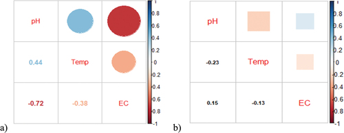
Correlation among water parameters and seasonality

Pearson correlation tests were conducted to measure the strength and extent of association between the water parameters investigated in this study and the season type (wet or dry). The Pearson correlation coefficients established for water parameters showed a weak, positive relationship between temperature and pH [p = 0.38, R = 0.44] in the dry season, while other associations showed negative correlations in both seasons (Figures 4a and 4b).

Figure 4. Correlation Matrix for Physicochemical Parameters of water in (a) dry season and (b) wet season.

Soil parameters

Soil texture and appearance

Soil samples collected from restored areas were composed of heavy clay (ribbon length: ≥75 mm, approximate clay content: ≥50%), while degraded mangrove ecosystems consisted of light, sandy clay (ribbon length: 50–75 mm, approximate clay content: 35–40%). However, the texture of soil samples collected from the natural mangrove ecosystems varied as sandy soils (ribbon length: nil, approximate clay content: <10%) were found in Novar, while heavy clayey soils (ribbon length: ≥75 mm, approximate clay content: ≥50%) were found in Hopetown. The soil textures in all three mangrove ecosystem types remained consistent in both wet and dry seasons.

pH, Salinity (EC), exchangeable acidity (EA), and organic carbon (OC)

Mangrove ecosystem type

One-way ANOVA (significance level: p < 0.05) results revealed insignificant differences in the means of OC, pH, EA, and EC found in the soil samples concerning ecosystem type.

Seasonality

Within the six mangrove areas, OC percentages ranged from 2.39–3.71% (DS) to 0.96–1.99% (WS). Furthermore, the mean EC values shifted from 1.16–1.29 mmhos/cm (DS) to 1.42 mmhos/cm (consistent in WS). pH values ranged on average between 6.45–7.338 (DS) and 6.49–7.338 (WS), while the EA of soils fluctuated between 0.09–0.22 (DS) and 0.09–0.12 meq/100 g soil (WS) (Table 3). However, the paired sample T-test revealed statistically significant differences between the two seasons in the mean values of OC [M = 1.46, t (5) = 4.53, p = 6.248e-03], EC [M = −0.19, t (5) = −8.51, p = 3.684e-04], and EA [M = 0.05, t (5) = 2.55, p = 0.05] among the three mangrove ecosystem types.

Table 3. Summary of results of OC, EC, pH and EA of soil samples (data expressed as Mean ± SEM).

Location	Ecosystem Type	Physicochemical Parameters of Mangrove Soil
		OC (%)		EC (mmhos/cm)		pH		EA (meq/100 g)
		Dry Season	Wet Season	Dry Season	Wet Season	Dry Season	Wet Season	Dry Season	Wet Season
Ogle	R	2.52 ± 0.13	1.49 ± 0.71	1.17 ± 0.25	1.42 ± 0.00	6.45 ± 0.06	6.66 ± 0.48	0.19 ± 0.06	0.12 ± 0.03
Montrose	R	3.59 ± 1.22	1.92 ± 0.90	1.29 ± 0.13	1.42 ± 0.00	6.65 ± 0.24	6.49 ± 0.03	0.16 ± 0.03	0.12 ± 0.03
Greenfield	D	2.39 ± 0.92	1.59 ± 0.46	1.20 ± 0.22	1.42 ± 0.00	7.13 ± 0.49	7.86 ± 0.59	0.22 ± 0.03	0.09 ± 0.00
Hope	D	3.71 ± 1.34	0.96 ± 0.45	1.28 ± 0.14	1.42 ± 0.00	7.26 ± 0.43	7.88 ± 0.70	0.09 ± 0.05	0.09 ± 0.00
Novar	N	2.92 ± 1.41	1.06 ± 0.27	1.25 ± 0.17	1.42 ± 0.00	7.38 ± 0.43	7.87 ± 0.55	0.16 ± 0.03	0.09 ± 0.00
Hopetown	N	2.91 ± 1.09	1.99 ± 0.00	1.16 ± 0.26	1.42 ± 0.00	7.33 ± 0.35	7.22 ± 0.56	0.09 ± 0.05	0.09 ± 0.00

Soil nutrient composition

Mangrove ecosystem type

A one-way ANOVA test, conducted at a significance level of p < 0.05, revealed statistically significant differences only in Mg concentration in the dry season only [F (5,17) = 14.94, p = 8.52e-05] among the three ecosystem types. Furthermore, a Tukey test on Mg concentrations (DS) [MSE = 0.02, Df = 12, M = 3.16, CV = 5.02, MSD = 0.43] further revealed that average Mg concentrations obtained from Montrose (R) (3.59 > 0.43), Ogle (R) (3.39 > 0.43), and Hope (D) (3.39 > 0.43) were similar to each other but differed significantly from Hopetown (N) (2.91 > 0.43), Greenfield (D) (2.88 > 0.43), and Novar (N) (2.78 > 0.43)(Table 4). Furthermore, the one-way ANOVA test also indicated significant differences in the mean Fe concentration values (DS only) (F (5,17) = 3.47, p = 0.04) in Novar (N), Montrose (R), Greenfield (D), and Hopetown (N) [Tukey Test: MSE = 0.14, Df = 12, M = 0.76, CV = 49.46, MSD = 1.02] (Table 5).

Table 4. Summary of Ca, Mg, S, N, and P concentrations found in soil samples (data expressed as Mean ± SEM).

Location	Ecosystem Type	Nutrient Composition of Mangrove Soils
		Ca (ppm)		Mg (ppm)		S (ppm)		N (ppm)		P (ppm)
		Dry Season	Wet Season	Dry Season	Wet Season	Dry Season	Wet Season	Dry Season	Wet Season	Dry Season	Wet Season
Ogle	R	2333.33 ± 405.52	4400.00 ±2107.13	2519.33^a ± 283.67	1382.67 ±247.37	269.24 ±76.53	357.51 ±226.94	16.19  ± 7.86	28.01 ±10.68	278.14 ±99.42	52.46 ±27.70
Montrose	R	2800.00 ± 923.76	3066.67 ±751.30	3944.67^a ± 317.62	2414.00 ±196.41	287.97 ±77.20	406.07 ±229.05	14.02  ± 7.50	25.63 ±6.63	298.75 ±113.61	169.61 ±97.97
Greenfield	D	3400.00 ± 1113.55	4200.00 ±503.32	813.33^b ± 162.67	1057.33 ±146.63	116.30 ±53.67	236.12 ±129.58	4.54  ± 4.54	11.55 ±4.57	147.17 ±27.92	55.51 ±24.85
Hope	D	6533.33 ± 2136.46	2533.33 ±371.18	2684^a ± 671.92	610.00 ±70.44	247.74 ±40.77	256.27 ±164.13	11.34 ± 5.93	12.19 ±3.93	303.15 ±94.85	243.22 ±209.61
Novar	N	3133.33 ± 569.60	3200.00 ±800.00	610.00^b ± 70.44	854.00 ±140.87	111.38 ±18.94	159.90 ±91.65	3.10 ±3.10	7.93 ±2.07	224.21 ±73.76	182.72 ±91.49
Hopetown	N	3066.67 ± 240.37	5000.00 ±1732.05	894.67^b ± 247.37	1342.00 ±865.54	209.99 ±36.89	257.62 ±225.72	6.40 ± 6.40	13.81 ±7.88	211.50 ±40.35	78.16 ±39.15

*Letters in table show significant pairwise associations using Tukey HSD Test.

Table 5. Summary of K, Zn, Mn, Cu, and Fe concentrations found in soil samples (data expressed as Mean ± SEM).

Location	Ecosystem Type	Nutrient Composition of Mangrove Soils
		K (ppm)		Zn (ppm)		Mn (ppm)		Cu (ppm)		Fe (ppm)
		Dry Season	Wet Season	Dry Season	Wet Season	Dry Season	Wet Season	Dry Season	Wet Season	Dry Season	Wet Season
Ogle	R	297.31 ±86.60	337.93 ±205.73	2.06 ±0.59	1.88 ±0.46	57.91 ±2.63	84.19 ±38.04	0.59 ±0.25	1.44 ±0.27	21.62^a ±7.27	11.00 ±2.29
Montrose	R	321.77± 88.34	435.73 ±208.47	2.33 ±0.89	2.80 ±0.43	65.41 ±2.28	61.55 ±34.61	0.44 ±0.08	1.01 ±0.25	11.83^ab ±2.98	9.72 ±2.08
Greenfield	D	116.30± 53.67	163.56 ±42.35	1.81 ±0.35	1.34 ±0.50	66.77 ±0.58	42.55 ±22.14	0.24 ±0.07	0.44 ±0.09	4.33^ab ±4.02	3.54 ±2.47
Hope	D	247.74± 40.77	120.77 ±27.01	0.55 ±0.26	1.45 ±0.62	75.90 ±17.20	31.51 ±14.94	0.09 ±0.05	1.67 ±0.50	0.60^b ±0.48	8.87 ±1.40
Novar	N	111.38± 18.94	144.91 ±45.71	2.60 ±0.68	1.94 ±0.78	85.85 ±14.12	30.90 ±15.57	0.58 ±0.24	1.85 ±0.96	13.54^ab ±4.96	10.06 ±4.34
Hopetown	N	209.99± 39.89	289.83 ±9.92	1.97 ±0.19	1.92 ±0.02	74.46 ±8.67	58.09 ±17.63	0.30 ±0.19	0.94 ±0.56	3.08^ab ±2.49	4.05 ±2.21

*Letters in table show significant pairwise associations using Tukey HSD Test.

Seasonality

Mean values of Ca ranged from 2800.00 ppm [Montrose (R)] – 6533.33 ppm [Hope (D)] in the dry season and 2533.33 ppm [Hope (D)] – 5000.00 ppm [Hopetown (N)] in the wet season, while average Mg concentrations ranged from 610.00 ppm [Novar (N)] – 3944.67 ppm [Montrose (R)] and 610.00 ppm [Hope (D)] – 2414.00 ppm [Montrose (R)] in the dry and wet seasons, respectively. Furthermore, S concentration values fluctuated between 111.38 ppm–287.97 ppm (DS) and 159.90 ppm–406.07 ppm (WS), with the lowest concentrations found in Novar (N) and highest in Montrose (R) (Table 4). Ca, Mg, and S concentrations of soils found in all six sites were above the critical limits (critical limits: Ca: 2500 ppm, Mg: 100 ppm, and S: >50 ppm) in both wet and dry seasons (Table 4). A paired T-test, conducted at a significance level of p < 0.05, confirmed significant differences [M = −0.14, t (5) = −3.54, p = 0.02] only between the average S concentrations in both seasons, among the different ecosystem types.

In addition, average nitrogen concentrations ranged from 3.10 ppm to 16.19 ppm (DS) to 7.93 ppm to 28.01 ppm (WS), with the lowest concentrations detected in Novar (N) and the highest in Ogle (R). Lower concentration values were present in soils found in natural and degraded mangrove ecosystems, while higher values were found in the restored mangrove stands (Table 4). Moreover, phosphorus concentration values [ranging from 147.17 ppm (Greenfield (D))−298.75 ppm (Montrose (R)) (DS) to 52.46 ppm (Ogle (R))−243.22 ppm (Hope (D)) (WS)] varied between mangrove ecosystems and seasons (Table 4). A similar trend was also observed with potassium concentrations in the dry season [111.38 ppm (Novar (N))–297.31 ppm (Ogle (R))] as well as the wet season [120.77 ppm (Hope (D))–337.93 ppm (Ogle (R))] among the three types of mangrove ecosystems (Table 5). In both wet and dry seasons, N, P, and K concentrations were above the critical limits (N: <240 ppm, P: >96 ppm, and K: >200 ppm), with restored ecosystems retaining higher concentrations of N and K (Table 4). However, paired T-tests (p < 0.05) conducted showed statistically significant differences in the mean concentrations of N [M = −0.25, t (5) = −5.14, p = 3.636e-03], P [M = 0.36, t (5) = 4.67, p = 5.48e-03] and K [M = 0.33, t (5) = 3.39, p = 0.02] between the two seasons.

Lastly, Zn concentration values ranged from 0.55–2.60 ppm (DS) to 1.34–2.80 ppm (WS), while Mn concentration values fluctuated between 57.91–85.85 ppm (DS) and 30.90–84.19 ppm (WS) among the ecosystem types (Table 5). Concentrations of copper found in the three different mangrove ecosystems varied from 0.09–0.59 ppm (DS) to 0.44–1.85 ppm (WS), while iron concentration values shifted from 0.60–21.62 ppm (DS) to 3.54–11.00 ppm (WS)(Table 5). Most mangrove sites had Zn, Cu, and Fe concentrations above the critical limits (Zn: 1.5 ppm, Cu: 0.2 ppm, Fe: 4.5 ppm), but Mn levels were moderately low (200 ppm) in both wet and dry seasons. Higher values for Fe were seen within restored and natural sites when compared to degraded sites. A paired T-test, on the other hand, revealed statistically significant differences (p < 0.05) in mean Cu concentrations in both wet and dry seasons [M = −0.20, t (5) = −4.49, p = 6.465e-03] (Table 5).

Correlation between soil parameters and seasonality

Like water parameters, Pearson correlation coefficients were also established to determine the strength of the association between soil parameters and seasonality. This was done to determine if soil parameters change in the same direction (+ve or -ve) concerning seasonality. In Figure 5a, it can be seen that in the dry season, the most significant positive correlations were observed between (in descending order): Cu~Fe (R = 0.97), N~Mg (R = 0.95), N~S (R = 0.95), Mg~K (R = 0.95), N~ EA (R = 0.93), Mg~S(R = 0.89), Mn~pH (0.89), Mn~N (R = 0.89), N ~ K (R = 0.86), Zn~Cu(R = 0.85), EA~S (0.84), Zn~Fe (R = 0.83), OC~K (R = 0.82), EA~K (R = 0.81), Mg~Zn (R = 0.80), S~K (R = 0.79) and S~ Mn (R = 0.79).

Figure 5. Cormatrix plots for soils parameters in the a) Dry Season and b) Wet season.

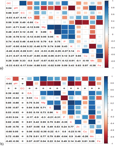
However, in the wet season, the number of positive associations increased between the parameters of soil when compared to the dry season. This can be seen in Figure 5b as the number of positive R values increased. It was also observed that the number of very strong positive associations between soil parameters decreased in the wet season when compared to the dry season. However, strong positive correlations were maintained by parameters such as EA and OC and nutrients such as (in descending order): Mg~K (R = 0.95), S~N (R = 0.95), EA~N (R = 0.93), Mn~K (R = 0.90), Mn~N (R = 0.89), N ~ K (R = 0.85), OC~Mg (R = 0.85), EA~S (R = 0.84), OC~K (R = 0.82), EA~K (R = 0.81), Cu~Fe (R = 0.81), S ~ K (R = 0.79), and S~Mn (R = 0.79).

Discussion

Water

The EC values obtained in this study showed seasonal variations that may be caused by the mobility of groundwater, water temperature, and soil rock leaching (Terungwa Temaugee et al., 2020). This may contribute to the fluctuating salinity levels caused by high temperatures and oceanic fluctuations, affecting mangrove trees and seedlings found in the various mangrove ecosystem types (Chowdhury et al., 2019). The pH levels observed in mangrove ecosystem water samples were within the appropriate range of 6.5–8.5, which is consistent with prior studies that recorded pH values in the range of 6.95–7.42 (Samara et al., 2020). Slight differences in pH levels among mangrove ecosystems may be due to ocean acidification and organic matter putrefaction (Dattatreya et al., 2018). Mangrove aerial roots have evolved to efficiently metabolise organic compounds from soils experiencing anoxia to release alkaline compounds into the waterways encroaching upon them. This stabilises the pH caused by increased carbon dioxide in the atmosphere and local waterways and facilitates the creation of equilibrium in open oceans (Thomas et al., 2017). Sippo et al. (2016) discovered that water surrounding the mangroves has a higher pH (8.1) than seawater farther away from the coastal mangroves (pH = 7.3). Such values are consistent with those reported only from natural mangrove ecosystems in this study. Cabañas-Mendoza et al. (2020) also showed that although the association was poor (R = 0.26 for A. germinans), elevations in the salt concentrations of a substrate may also cause an increase in the pH of water in mangrove areas.

Findings for the correlation between pH and EC were based on results obtained by Dattatreya et al. (2018), which showed no significant relationship between the two parameters. In most circumstances, EC shows a greater relationship with temperature than pH (Oyem et al., 2014). However, the correlation between EC and temperature was not consistent with results from other research (Rusydi , 2018; Tyler et al., 2017), which indicated that temperature has a direct effect on the electrical conductivity of water. The findings in this study showed a weak, negative relationship between the two parameters. A possible explanation for the inverse relationship showcased between temperature and EC was offered by Schmidt et al. (2018), who posited that the temperature and density of saltwater (oceanic in nature) are inversely proportional. As the temperature rises, the space within water molecules expands, causing the density to decrease. He also noted that salinity (demonstrated in this study as measurements of electrical conductivity) and density share a positive relationship. As a result, as water’s temperature drops, its density rises, but only to a limit. Findings on the various relationships between the physicochemical parameters of water in this study provide further evidence that the relationships between pH, temperature, and EC may be affected by many factors, some of which are reflected in differences within the environmental setting of various mangrove ecosystems, which encompasses their hydrological framework and patterns, including tidal wave impacts, riverine forces and influences, groundwater flow, and surface runoffs from highlands (Li et al., 2008). Wan et al. (2014) and Atwell et al. (2016) also confirmed that tidal inundation is a key determinant of abiotic variables including salinity, physicochemical properties of water, and redox potential. Climate change, water degradation, contamination, changes in water flow, groundwater, and light regimes are all examples of factors that affect the physicochemical characteristics of water resulting from anthropogenic activities ([EPA] Environmental Protection Agency, 2018).

Soils

Texture and appearance

Despite variations in soil texture and appearance of soil samples collected in the three mangrove ecosystems, the soil textures recorded in this study were consistent with other research on mangrove soils, which revealed that mangrove soil surfaces are mostly composed of freshly deposited sediment particles and are known as sandy or silty loams (Andrade et al., 2018; Bomfim et al., 2018). Furthermore, Moreno and Calderon (2011) discovered that within mangrove forests, the soil is partly composed of sand, clay, and loam with 53.17% of the total comprising sand particles. Silty clay is primarily found in logged and undisturbed mangroves, though some species may prefer different types of soil. However, moving towards the seaward zone, Avicennia sp. can be detected on sandy soils (Ibrahim & Hossain, 2012; Sofawi, 2017). This zonation pattern was evident within the degraded areas of this study as the soils found in these areas were mostly composed of sand.

pH, salinity (EC), exchangeable acidity (EA), and organic carbon (OC)

In this study, results showed significant differences in percentages of EC, EA, and OC concerning seasonality but not ecosystem type. Mangroves are well known for their abundant carbon stores and high rates of carbon sequestration in soil and biomass (Rovai et al., 2022). The OC percentages obtained in this research are consistent with those obtained by Matsui et al. (2015), in which OC percentages are usually higher in the wet seasons than in the dry seasons (Kathiresan et al., 2014). However, Georgiadis et al. (2017) and Lei et al. (2019) confirmed that many factors could influence seasonal variations in OC levels in the soil. Such factors would include land use, species of plants, site characteristics (slope and location), underlying soil properties, stand age, microbial activity, and species density (Babur & Dindaroglu, 2020; Sofawi, 2017). Climate change (such as water temperature elevations) and anthropogenic activities such as logging, pollution, and land-use conversions, along with insect invasion, are all factors that affect mangrove SOC in different mangrove ecosystem types (Gao et al., 2019). While it was not evident within this study, studies have shown that OC % is usually higher in mature forests and two times greater in replanted forests when compared to non-vegetative soils due to enrichment provided by litter fall and stored carbon content in vegetation (Kathiresan et al., 2014).

Shahid et al. (2014) and Alsumaiti and Shahid (2018) describe electrical conductivity (EC) as a parameter that indirectly serves as an indicator of soil salinity and can be considered a key component of soil health. Jeyanny et al. (2018) reported EC values of 11.99 ms/cm in regenerating mangrove ecosystems and 20.92 ms/cm in established mangrove ecosystems. These values are significantly higher when compared to the values observed in this study. However, Sudduth et al. (2005) and Kida et al. (2017) observed that the physical and biological characteristics of soil, including soil type, organic compounds, moisture and temperature of the soil, and Cation Exchange Capacity (CEC), can influence soil EC readings, thus creating significant soil EC variations. The evaporation and evapotranspiration over the salt flats and mangroves may cause rapid increases in salinity and may cause variations during dry and wet seasons (Komiyama et al., 2019). Variations in EC values between seasons (wet and dry) can also be due to instances where the origin of the water among mangroves may not be seawater. This was further clarified by research conducted by Lambs et al. (2008) on black mangroves found in French Guiana, in which the groundwater can acquire a salty nature which is mainly caused by the seepage of freshwater from marshes found inland and stormwater in the rainy season, which causes marine evaporite to be dissolved repeatedly. Furthermore, they have also confirmed that seasonal patterns, transpiration, and the presence of freshwater influx influence salinity changes in the upper sediment of mangrove soils. This affects the accumulation of salt under the mangrove forest, causing the formation of brine during the dry season. This will subsequently dissolve in the wet season, owing to the natural convection processes.

Soil pH values in this study ranged from 6.45 to 7.88, which were considered to be within a neutral pH range and were consistent with values obtained by Bomfim et al. (2015), Tran Thi (2018), and Andrade et al. (2018). The neutrality of the pH of mangrove soils in varying seasons (evident in this study) was explained by Hseu and Chen (2012) as the impact of seawater on the mangrove areas. Mangroves can flourish at their optimum rate even with a soil pH level of 5.16 to 7.72, according to Lim et al. (2012), so they can adjust themselves to withstand adverse environmental conditions and lower nutritional accessibility. However, young mangrove seedlings, particularly those in the early growth stages, cannot withstand severe pH conditions (>5.16–7.72) since they prevent nutrients from reaching the plants (Alsumaiti & Shahid, 2018). The low EA values found in this analysis were similar to those found by Adamu et al. (2014), while Onwuka et al. (2016) found that hydrogen, sulphate, iron, and aluminium ions were the key factors influencing soil exchangeable acidity when soil pH is low. Therefore, soils present within the mangrove sites in this study do not need to be neutralised to buffer their pH since their values (corresponding to low EA values) were within an acceptable range.

Nutrient composition

Sulphur concentrations reported in this study were sufficient in mangrove soils and showed no significant differences among locations. This was consistent with results obtained by Madi et al. (2015) in similar mangrove stands found in Brazil. However, sulphur concentrations varied among the seasons within the six mangrove stands, with elevated values in the wet season when compared to the dry. Studies conducted by Hofer (2018) and Jørgensen et al. (2019) showed that microorganisms are considered to be the primary source of sulphur oxidation and reduction, although in numerous cases, chemical reactions such as organic matter degradation are included. The sulphur cycle, and thus the rate of soil sulphur oxidation, is influenced by environmental conditions such as pH, temperature, moisture, microbial activity, organic material, particle size, and atmospheric pollution. Reduced water supply encourages aeration of the soil, degradation, and depletion of metal sulphides from mangrove soils, mostly during the dry season (Nóbrega et al., 2013). Seasonal fluctuations in forms of sulphur found in mangroves suggest that seasonal weather conditions may affect geochemical processes in these ecosystem types.

The results of this study, being consistent with results obtained by Rivera-Monroy et al. (2004) and Khan and Amin (2019), confirmed that Ca concentrations are sufficient in the soils and show no significant differences between mangrove locations or seasons. However, when calcium is (1) dissolved or extracted from irrigation water, (2) extracted by plants, (3) ingested by organisms in the soil, (4) removed from the soil by rain, or (5) taken in by clayey particles, variations in the concentration of available calcium in the soil may occur (Oldham, 2019). Not much is known about the Ca content of mangrove soils in Guyana. However, based on observations made within the various mangrove ecosystems, the high Ca content found within the soils may be due to organism ingestion (crabs) as well as the presence of broken shells, which can increase the CaCO₃ content within the soils (Andrade et al., 2018).

Furthermore, an examination of the results obtained from the Mg concentrations showed that there were sufficient amounts of Mg present within all six sites, with differences in locations but not seasons. The values obtained were consistent with studies conducted by Motamedi et al. (2014) and Windusari et al. (2014). Similar results were also obtained by Gutiérrez (2016), who reported increased amounts of Mg in low-disturbance mangrove ecosystems, and small concentrations were detected in mangrove stands with high disturbances. Such variations in Mg can be caused by strong tidal rhythms owing to the mixing of estuarine and mangrove waters, salinity, and primary aquatic productivity (Manju et al., 2012).

The findings of this study are consistent with those of Madi et al. (2015), who showed no significant differences between NPK levels in the mangrove soils found in the six different study sites. However, there were marked differences between seasons, with concentrations fluctuating between the different locations and with values of nitrogen and phosphorus being low in most sites. During wet periods, certain soil nutrients may be more easily accessible than during dry periods, according to Sonko et al. (2016), who pointed out that the moisture content in the wet season subsequently promotes soil nutrient availability for plant root absorption. Low water availability slows down decomposition and biogeochemical cycles because the water film surrounding soil particles prevents nutrients and enzymes from diffusing into the soil, which limits the amount of substrate available for microorganisms (Guntiñas et al., 2013; Xue et al., 2017). Alsumaiti and Shahid (2018) explain that low phosphorus availability and efficiency in mangrove soils may be due to phosphorus fixation with high CaCO₃ levels, which may result in reduced P accessibility and efficiency in plants unless the release of fixed phosphorus is aided by acidic conditions.

Furthermore, low N levels in the soil may be due to denitrifying bacteria being prevalent within mangrove soils, resulting in high rates of denitrification owing to anaerobic environmental conditions and high OM content, which in turn causes a lowering of nitrogen levels (Alfaro-Espinoza & Ullrich, 2015; Pupin & Nahas, 2014). As a result of the high accumulation of cations in ocean water competing for binding sites, absorption of ammonium by soil particles in mangrove areas is generally poorer when compared to terrestrial habitats, rendering ammonium accessible for plant roots to absorb (Reef et al., 2010). High K concentrations obtained in this study were consistent with results obtained by Sofawi (2017) and Alsumaiti and Shahid (2018), who concluded that there are two major explanations for the high potassium content in the soil: a) mud rich in organic material and accumulation of deteriorated organic matter over time by pneumatophores, which facilitate potassium release into the soil (located in areas that have low disturbance and are minimally affected by humans); and b) potassium is found in the crystal structure of minerals like K-feldspar and mica, which release it during weathering (Reef et al., 2010).

Cuzzuol and Rocha (2012) and Madi et al. (2015) give explanations for dissimilarities in the proportions of Mn, Zn, Cu, and Fe in soils, both between species and mangroves, which may be due to variations (spatially and temporally) as well as physicochemical soil properties. Earlier studies conducted by D. Alongi (2018) and Taillardat et al. (2019) further explained that tidal variations can also interfere with the availability of chemical elements, which could result in the alterations of the nutrient concentrations present in various mangrove ecosystems. This was observed in the differences between Cu concentrations, with higher concentration values in the wet season when compared to the dry season. Fluctuations of Fe were detected among the six mangrove ecosystems, with natural and restored mangrove ecosystems having the most significant differences and higher concentrations when compared to degraded mangrove ecosystems, which showcased low Fe levels in the soils. It has been observed that manmade irrigation structures located at Hope and Greenfield (degraded mangrove stands) cause frequent flooding of the area due to the size of the structures, which may interfere with incoming and outgoing tidal patterns. This may provide a possible explanation for the reduced Fe concentrations in degraded mangrove soils since high levels of water promote the leaching of nutrients. Differences in Fe concentrations may also be caused by variations in sediment origin because seasonal waterlogging causes Fe to accumulate in clay-rich soils. However, a build-up of organic detritus and Fe-rich soil particles in streams allows Fe to be released under anaerobic conditions and then bound by organic matter (Löhr et al., 2010).

In this study, Mn concentrations were below the critical limit in all mangrove sites. Mn insufficiency is brought on by two different inadequacies: those caused by chemical factors in the soil and those associated with biological factors. Between seasons, areas that fluctuate between well-drained and waterlogged conditions may develop manganese deficiencies due to constant flow between the mangrove forest sediments and tidal water (Alongi, 2021). This is usually observed within mangrove forests along the coastline since they experience rapid tidal inundations. As they lead to Mn accumulation and may be actively engaged in retaining its level as well as other associated metal quantities like Fe among mangrove sites, both autochthonous heterotrophs and autotrophs work cohesively to mitigate Mn and associated metals such as Fe within mangrove swamps (Krishnan et al., 2007).

Correlations between nutrient concentrations and seasonality

Examination of the correlation values within the correlation matrices for wet and dry seasons shows complex and significant associations between soil nutrients and other physicochemical parameters. Such fluctuations are thought to be directly linked to the accumulation of nutritionally rich silt during the rainy season, followed by depletion due to plant absorption and tidal leaching at various periods throughout the year (Sofawi, 2017). The results derived from this study show consistency with earlier studies (Fernandes et al., 2013; Rahaman et al., 2013) that have shown strong positive correlations between nutrient concentrations in mangrove soils, in which they have indicated that changes in hydroperiods, as well as leaf litter quantity and quality within mangrove stands, can cause seasonal patterns of nutrient immobilisation. Furthermore, Numbere (2019) reported that the concentration of metals and nutrients in mangrove soils can vary in seasons, with emissions from anthropogenic activities identified as the key source.

Conclusion

This study focused on the physicochemical parameters of water and soil found in natural, degraded, and restored mangrove ecosystems in Guyana, concerning ecosystem type as well as seasonality. Our results did not show significant variations in most of the physicochemical parameters of soil and water between the natural, restored, and degraded areas. However, notable differences were seen in the pH of water as well as Fe and Mg concentrations of soil within the three types of ecosystems. Additionally, seasonal differences were also evident in S, N, P, K, and Cu concentrations found within the mangrove soils. In both seasons, positive correlations were evident among soil parameters, while negative correlations were established among the water parameters investigated in this study. The findings of this study suggest that though variations exist, the physicochemical parameters of soil and water found within the mangrove ecosystems along Guyana’s coastline are not heavily influenced by ecosystem type (natural, degraded, or restored) or seasonality (wet and dry periods).

Geolocation information

Study locations in Guyana (SA) with GPS Coordinates:

1. Ogle, Georgetown (Region 4): 6.82349, −58.09528

2. Montrose, Georgetown (Region 4): 6.82024, −58.07688

3. Hope, East Coast Demerara (Region 4): 6.74644, −57.95619

4. Greenfield, East Coast Demerara (Region 4): 6.73843, −57.94596

5. Novar, East Coast Demerara (Region 5): 6.56846, −57.76294

6. Hopetown, West Coast Berbice (Region 5): 6.40364, −57.59729

Acknowledgments

The authors would like to express gratitude to the Department of Biology, Centre for the Study of Biological Diversity (CSBD) (UG), World Wildlife Fund Guianas, and National Agricultural Research and Extension Institute (NAREI) for their valuable contributions.

Disclosure statement

No potential conflict of interest was reported by the author(s).

Additional information

Funding

This work was supported by the WWF Guianas under Grant number UGUFWWF0017; and National Agricultural Research and Extension Institute (NAREI) under Grant number NAREI/2020-01.

References

- Ackroyd, ca. 2010. Final report of the mangrove technical assistance for capacity building and institutional strengthening of the sea defences sector -, EDF 2007 Europe Aid/127405/D/SER/GY.
- Adamu, U., Muhammad, A., & Adam, I. (2014). Evaluation of soil reaction, exchangeable acidity and cation exchange capacity of soils from kano university of science and technology wudil teaching, research and commercial farm, Gaya. Bayero Journal of Pure and Applied Sciences, Internet]. [accessed. 7(1), 52. https://doi.org/10.4314/bajopas.v7i1.10
- Ahmad, R. S., & Lakhan, C. (2012). GIS-Based analysis and modelling of coastline advance and retreat along the coast of Guyana. Marine Geodesy, 35 (1), 1–15. [accessed 2022 Oct 10, Internet https://www.tandfonline.com/doi/full/10.1080/01490419.2011.637851
- Alappatt, J. P. (2008). Structure and species diversity of mangrove ecosystem. biodiversity and climate change adaptation in tropical islands. Internet]. [accessed. 127–144. https://doi.org/10.1016/b978-0-12-813064-3.00005-3
- Alfaro-Espinoza, G., & Ullrich, M. S. (2015). Bacterial N2-fixation in mangrove ecosystems: Insights from a diazotroph–mangrove interaction. Frontiers in Microbiology, Internet]. [accessed. 6. https://doi.org/10.3389/fmicb.2015.00445
- Aljahdali, M. O., Alhassan, A. B., & Zhang, Z. (2021). Environmental factors causing stress in avicennia marina mangrove in rabigh lagoon along the red sea: based on a multi-approach study. Frontiers in Marine Science, Internet]. [accessed. 8, https://doi.org/10.3389/fmars.2021.646993
- Almahasheer, H., Duarte, C. M., & Irigoien, X. (2016). Nutrient Limitation in Central Red Sea Mangroves. Frontiers in Marine Science, Internet]. [accessed. 3. https://doi.org/10.3389/fmars.2016.00271
- Almahasheer, H., Serrano, O., Duarte, C. M., & Irigoien, X. (2018). Remobilization of heavy metals by mangrove leaves. Frontiers in Marine Science, Internet]. [accessed. 5, https://doi.org/10.3389/fmars.2018.00484
- Alongi, D. (2018). Impact of global change on nutrient dynamics in Mangrove forests. Forests, Internet]. [accessed. 9(10), 596. https://doi.org/10.3390/f9100596
- Alongi, D. M. (2020). Nitrogen cycling and mass balance in the world’s Mangrove forests. Nitrogen, Internet]. [accessed. 1(2), 167–189. https://doi.org/10.3390/nitrogen1020014
- Alongi, D. M. (2021). Macro- and micronutrient cycling and crucial linkages to geochemical processes in Mangrove Ecosystems. Journal of Marine Science and Engineering, Internet]. [accessed. 9(5), 456. https://doi.org/10.3390/jmse9050456
- Alongi, D. M., & Gouissem, I. (2015). The Impact of Climate Change on Mangrove Forests. Current Climate Change Reports. ARP Rheumatology, 1(1), 30–39. [accessed 2022 Oct 5. Internet. https://doi.org/10.1007/s40641-015-0002-x
- Alsumaiti, T. S., & Shahid, S. A. (2018). A comprehensive analysis of Mangrove Soil in Eastern Lagoon National Park of Abu Dhabi Emirate. IJBASS, 4(5), 39–55. https://nbn-resolving.org/urn:nbn:de:0168-ssoar-57449-3
- Andrade, K. V., Holanda, F. S., Santos, T. D., Santana, M. B., & Araújo Filho, R. N. (2018). Mangrove soil in physiographic zones in the Sao Francisco River estuary. Floresta E Ambiente, 25(2). https://doi.org/10.1590/2179-8087.063816
- Atwell, M. A., Wuddivira, M. N., & Gobin, J. F. (2016). Abiotic water quality control on mangrove distribution in estuarine river channels assessed by a novel boat-mounted electromagnetic induction technique. Water SA, 42(3), 399. [accessed 2021 May 14. Internet. https://doi.org/10.4314/wsa.v42i3.04
- Babur, E., & Dindaroglu, T. (2020). Seasonal changes of Soil Organic Carbon and Microbial Biomass Carbon in Different Forest Ecosystems. Ed., Environmental Factors Affecting Human Health. IntechOpen, Internet] [accessed 2022 September 13 https://doi.org/10.5772/intechopen.90656
- Bharati, D. 2019. Methods of Sampling Plant Communities. Biology Discussion [Internet]. [accessed 2021 May 14]. https://www.biologydiscussion.com/plant-ecology/methods-of-sampling-plant-communities/57189
- Bomfim, M. R., Santos, J. A., Costa, O. V., Conceiçao, J. N., Silva, A. A., Souza, C. D., & Almeida, M. D. (2018). Morphology, Physical and Chemical Characteristics of Mangrove Soil under Riverine and Marine Influence: A Case Study on Subaé River Basin, Bahia, Brazil. Mangrove Ecosystem Ecology and Function. https://doi.org/10.5772/intechopen.79142
- Bomfim, M. R., Santos, J. A. G., Costa, O. V., Otero, X. L., Boas, G. D., Capelão, S. V., Santos E de S Dos, V. D. S., & Nacif, P. G. S. (2015). Genesis, characterization, and classification of Mangrove Soils in the Subaé River Basin, Bahia, Brazil. Revista Brasileira de Ciência do Solo, Internet]. [accessed. 39(5), 1247–1260. https://doi.org/10.1590/01000683rbcs20140555
- Boto, K. G. (2018). Nutrients and mangroves pollution in tropical aquatic systems. Internet]. [accessed. 129–145. https://doi.org/10.1201/9781351075879-5
- Broadley, M., Brown, P., Cakmak, I., Rengel, Z., & Zhao, F. (2012). Function of Nutrients. Marschner's Mineral Nutrition of Higher Plants, 191–248. https://doi.org/10.1016/b978-0-12-384905-2.00007-8
- Cakmak, I. (2013). Magnesium in crop production, food quality and human health. Plant and Soil, Internet]. [accessed. 368(1–2), 1–4. https://doi.org/10.1007/s11104-013-1781–2
- Cardinale, B. J., Srivastava, D. S., Emmett Duffy, J., Wright, J. P., Downing, A. L., Sankaran, M., & Jouseau, C. (2006). Effects of biodiversity on the functioning of trophic groups and ecosystems. Nature, Internet]. [accessed. 443(7114), 989–992. https://doi.org/10.1038/nature05202
- Carugati, L., Gatto, B., Rastelli, E., Lo Martire, M., Coral, C., Greco, S., & Danovaro, R. (2018 [accessed 2022 Oct 5). Impact of mangrove forests degradation on biodiversity and ecosystem functioning. Scientific Reports, 8(1). Internet. https://doi.org/10.1038/s41598-018-31683-0.
- Chowdhury, R., Sutradhar, T., MstM, B., Mukherjee, C., Chatterjee, K., Basak, S. K., & Ray, K. (2019). Effects of nutrient limitation, salinity increase, and associated stressors on mangrove forest cover, structure, and zonation across Indian Sundarbans. Hydrobiologia, 842(1), 191–217. [accessed 2022 Oct 4]. Internet. https://doi.org/10.1007/s10750-019-04036-9
- Cuzzuol, G. R. F., & Rocha, A. C. (2012). Interação do regime hídrico com as relações nutricionais em ecossistema manguezal. Acta Botanica Brasilica, Internet]. [accessed. 26(1), 11–19. https://doi.org/10.1590/s0102-33062012000100003
- Dattatreya, P. S., Madhavi, K., Satyanarayana, B., Amin, A., & Harini, C. (2018). Assessment of Physicochemical characteristics of Mangrove region in THE Krishnapatnam Coast, India. IJCMAS, 7(5), 2326–2342. https://doi.org/10.20546/ijcmas.2018.705.268
- Del R Cabañas-Mendoza, M., Santamaría, J. M., Sauri-Duch, E., Escobedo-GraciaMedrano, R. M., & Andrade, J. L. (2020). Salinity affects pH and lead availability in two mangrove plant species. Environmental Research Communications, Internet]. [accessed. 2(6), 061004. https://doi.org/10.1088/2515-7620/ab999
- Dewiyanti, I., Darmawi, D., Muchlisin, Z. A., Helmi, T. Z., Imelda, I., & Defira, C. N. (2021). Physical and chemical characteristics of soil in mangrove ecosystem based on different habitats in Banda Aceh and Aceh Besar. IOP Conference Series: Earth and Environmental Science, Internet]. [accessed. 674(1), 012092. https://doi.org/10.1088/1755-1315/674/1/012092
- Dissanayake, N., & Chandrasekara, U. (2014). Effects of Mangrove Zonation and the Physicochemical Parameters of Soil on the Distribution of Macrobenthic Fauna in Kadolkele Mangrove Forest, a Tropical Mangrove Forest in Sri Lanka. Advances in Ecology, Internet]. [accessed. 1–13. https://doi.org/10.1155/2014/564056
- Dm, H., Carpenter, K. E., Collins, L., Duke, N. C., Ellison, A. M., Ellison, J. C., Farnsworth, E. J., Fernando, E. S., Kathiresan, K., Koedam, N. E., Livingstone, S. R., Miyagi, T., Moore, G. E., Ngoc Nam, V., Ong, J. E., Primavera, J. H., Salmo, S. G., Sanciangco, J. C., Sukardjo, S., & Yong, J. W. H. (2010). The Loss of Species: Mangrove Extinction Risk and Geographic Areas of Global Concern. D. M. Hanseneditor, PLoS ONE, Internet]. [accessed, 5(4), e10095. https://doi.org/10.1371/journal.pone.0010095
- Dookie, S., Jaikishun, S., & Abdullah, A. A. (2022). A comparative study of mangroves in degraded, natural, and restored ecosystems in Guyana. Biodiversity, 23(2), 40–48. https://doi.org/10.1080/14888386.2022.2107570
- Dookram, K., Jaikishun, S., Ansari, A., & Seecharran, D. (2017). A Comparison of the Effects of Mangrove Ecosystems (Disturbed and Undisturbed) on the Populations of Birds and Fishes at Hope Beach, East Coast Demerara, Region 4, Guyana. International Journal of Agricultural Technology, 13(3), 331–342. https://www.researchgate.net/publication/319236716
- [EAME] Earth and Marine Environmental Consultants. (2018). North Brazil Shelf Mangrove Project Mangrove Cover of Guyana. Fron Fawr Farm. Wales, UK: Earth and Marine Environmental Consultants.
- [EPA] Environmental Protection Agency. 2009. Field Sampling Guidance Document – Soil Sampling [Internet]. [accessed 2021 May 13] https://dehs.umn.edu/sites/dehs.umn.edu/files/19990901
- [EPA] Environmental Protection Agency. 2018. Report on the Environment: Physical and Chemical Attributes [Internet]. [accessed 2021 February 26] https://www.epa.gov/report-environment/physical-and-chemical-attributes
- Fageria, N. K. (2008). The Use of Nutrients in Crop Plants. CRC Press. Boca Raton.
- Fernandes, S. O., Gonsalves, M.-J., Michotey, V. D., Bonin, P. C., & LokaBharathi, A. (2013). Denitrification activity is closely linked to the total ambient Fe concentration in mangrove sediments of Goa, India. Estuarine, Coastal and Shelf Science, Internet]. [accessed. 131, 64–74. https://doi.org/10.1016/j.ecss.2013.08.008
- Friess, D. A., Rogers, K., Lovelock, C. E., Krauss, K. W., Hamilton, S. E., Lee, S. Y., Lucas, R., Primavera, J., Rajkaran, A., & Shi, S. (2019). The State of the World’s Mangrove Forests: Past, Present, and Future. Annual Review of Environment and Resources, 44(1), 89–115. https://doi.org/10.1146/annurev-environ-101718-033302
- Gao, Y., Zhou, J., Wang, L., Guo, J., Feng, J., Wu, H., & Lin, G. (2019). Distribution patterns and controlling factors for the soil organic carbon in four mangrove forests of China. Global Ecology and Conservation, Internet]. [accessed. 17, e00575. https://doi.org/10.1016/j.gecco.2019.e00575
- Georgiadis, P., Vesterdal, L., Stupak, I., & Raulund-Rasmussen, K. (2017). Accumulation of soil organic carbon after cropland conversion to short-rotation willow and poplar. GCB Bioenergy, Internet]. [accessed. 9(8), 1390–1401. https://doi.org/10.1111/gcbb.12416
- Getzner, M., & Islam, M. S. (2020). Ecosystem Services of Mangrove Forests: Results of a Meta-Analysis of Economic Values. International Journal of Environmental Research and Public Health, Internet]. [accessed. 17(16), 5830. https://doi.org/10.3390/ijerph17165830
- Gumpili, S. P., & Das, A. V. (2022). Sample size and its evolution in research. IHOPE Journal of Ophthalmology, Internet]. [accessed. 1, 9–13. https://doi.org/10.25259/ihopejo_3_2021
- Guntiñas, M. E., Gil-Sotres, F., Leirós, M. C., & Trasar-Cepeda, 2013. Sensitivity of soil respiration to moisture and temperature Journal of Soil Science and Plant NutritionInternet]. [accessedaheadhttps://doi.org/10.4067/s0718-95162013005000035
- Gutiérrez, J. C. (2016). Comparison of the mangrove soil with different levels of disturbance in tropical agua Brava Lagoon, Mexican Pacific. Applied Ecology and Environmental Research, 14(4), 45–57. https://doi.org/10.15666/Aeer/1404_045057
- Guyana Forestry Commission, G. F. C. (2011). Guyana National Forestry Policy Statement.
- Guyana Forestry Commission, G. F. C. 2017. Sector Information Report: Annual Review [Internet]. Guyana Forestry Commission (GFC) under the Department of Environment (DOE). [accessed 2022 September 18] https://www.doe.gov.gy/published/document/5d122186e571586f465b1b27
- Hacisalihoglu, G. (2020). Zinc (Zn): the last nutrient in the alphabet and shedding light on zn efficiency for the future of crop production under suboptimal Zn. Plants, Internet]. [accessed. 9(11), 1471. https://doi.org/10.3390/plants9111471
- Harahap, N., Lestariadi, R. A., & Soeprijanto, A. (2015). The effect of soil quality on the survival rate of mangrove vegetation. Journal of Engineering and Applied Sciences, 10(7), 154–156. https://doi.org/10.3923/jeasci.2015.154.156
- Hayes, M. A., Jesse, A., Welti, N., Tabet, B., Lockington, D., & Lovelock, C. E. (2018). Groundwater enhances above‐ground growth in mangroves.Wurzburger N, editor. Journal of Ecology, 107(3), 1120–1128. [accessed 2022 Sep 8. Internet. https://doi.org/10.1111/1365-2745.13105
- Hofer, U. (2018). New diversity in the sulfur cycle. Nature Reviews. Microbiology, Internet]. [accessed. 16(5), 261. https://doi.org/10.1038/nrmicro.2018.32
- Hogarth, P. J. (2015). The Biology of Mangroves and Seagrasses. Oxford University Press. The UK.
- Hossain, M. D., & Nuruddin, A. A. (2016). Soil and Mangrove: A Review. Journal of Environmental Science and Technology, 9 (2), 198–207. [accessed 2022 Sep 7, Internet https://scialert.net/abstract/?doi=jest.2016.198.207
- Hseu, Z. Y., & Chen, Z. S. (2012). Monitoring the changes of redox potential, pH and electrical conductivity of the mangrove soils in northern Taiwan. Proceedings of the National Science Council, Republic of China. Proceedings of the National Science Council, Republic of China, 24(3). https://pubmed.ncbi.nlm.nih.gov/10943948/
- Ibrahim, S., & Hossain, L. (2012). Mangroves of Terengganu (2nd.) ed.). Penerbit Universiti Malaysia Terengganu.
- Jaikishun, S., Ansari, A., Da Silva, P., & Hosen, A. (2017). Carbon storage potential of mangrove forest in Guyana. Bonorowo Wetlands, 7(1). https://doi.org/10.13057/bonorowo/w070109
- Jeyanny, V., Siva Kumar, B., Ne’ryez, S. R., Fakhri, M. I., Daljit, S. K., Maisarah, M. Z., Wan Rasidah, K., & Husni, M. H. A. (2018). Assessing soil quality of a regenerating Mangrove Forest using geospatial modelling approach. Malaysian Journal of Soil Science, 22, 161–173. http://www.msss.com.my/./V22_11.pdf
- Jørgensen, B. B., Findlay, A. J., & Pellerin, A. (2019). The Biogeochemical sulfur cycle of marine sediments. Frontiers in Microbiology, Internet]. [accessed. 10. https://doi.org/10.3389/fmicb.2019.00849
- Kannappan, T., Shanmugavelu, M., & Karthikeyan, M. M. (2012).Internet] [accessed 2020 October 04 Concentration on heavy metals in sediments and mangroves from Manakudy Estuary (South West Coast of India). European Journal of Biology, 4, 109–113. https://doi.org/10.5829/idosi.ejbs.2012.4.4.1103
- Kathiresan, K., Gomathi, V., Anburaj, R., & Saravanakumar, K. (2014). Impact of mangrove vegetation on seasonal carbon burial and other sediment characteristics in the Vellar-Coleroon estuary, India. Journal of Forestry Research, Internet]. [accessed. 25(4), 787–794. https://doi.org/10.1007/s11676-014-0526-2
- Khairnar, S. O., Sathe, A. R., Mhatre, V. D., Jadhav, S. S., & Desai, K. B. (2009). Mangrove Biodiversity of India. Aqua International, 16(12), - 29–30.
- Khan, M., & Amin, M. (2019). Macronutrient status of Sundarbans forest soils in Southern region of Bangladesh. Bcsir, Internet]. [accessed. 54(1), 67–72. https://doi.org/10.3329/bjsir.v54i1.40732
- Kida, M., Tomotsune, M., Iimura, Y., Kinjo, K., Ohtsuka, T., & Fujitake, N. (2017). High salinity leads to the accumulation of soil organic carbon in mangrove soil. Chemosphere, 177, 51–55. https://doi.org/10.1016/j.chemosphere.2017.02.074
- Kodikara, K. A. S., Jayatissa, L. P., Huxham, M., Dahdouh-Guebas, F., & Koedam, N. (2017). The effects of salinity on the growth and survival of mangrove seedlings change with age. Acta Botanica Brasilica, Internet]. [accessed. 32(1), 37–46. https://doi.org/10.1590/0102-33062017abb0100
- Komiyama, A., Poungparn, S., Umnouysin, S., Rodtassana, C., Pravinvongvuthi, T., Noda, T., & Kato, S. (2019). Occurrence of seasonal water replacement in mangrove soil and the trunk growth response of Avicennia alba related to salinity changes in a tropical monsoon climate. Ecological Research, Internet]. [accessed. 34(3), 428–439. https://doi.org/10.1111/1440-1703.12005
- Krauss, K. W., McKee, K. L., Lovelock, C. E., Cahoon, D. R., Saintilan, N., Reef, R., & Chen, L. (2013). How mangrove forests adjust to rising sea levels. New Phytologist, Internet]. [accessed. 202(1), 19–34. https://doi.org/10.1111/nph.12605
- Krishnan, K. P., Fernandes, S. O., Chandan, G. S., & Loka Bharathi, P. A. (2007). Bacterial contribution to mitigation of iron and manganese in mangrove sediments. Marine Pollution Bulletin, Internet]. [accessed. 54(9), 1427–1433. https://doi.org/10.1016/j.marpolbul.2007.05.023
- Lambs, L., Muller, E., & Fromard, F. (2008). Mangrove trees growing in a very saline condition but not using seawater. Rapid Communications in Mass Spectrometry, Internet]. [accessed. 22(18), 2835–2843. https://doi.org/10.1002/rcm.3676
- Lawrence, P. G., Roper, W., Morris, T. F., & Guillard, K. (2020). Guiding soil sampling strategies using classical and spatial statistics: A review. Agronomy Journal, Internet]. [accessed. 112(1), 493–510. https://doi.org/10.1002/agj2.20048
- Lee, S. Y., Primavera, J. H., Dahdouh-Guebas, F., McKee, K., Bosire, J. O., Cannicci, S., Diele, K., Fromard, F., Koedam, N., Marchand, C., et al. (2014). Ecological role and services of tropical mangrove ecosystems: A reassessment. Global Ecology and Biogeography, 23(7), 726–743. https://doi.org/10.1111/geb.12155
- Lei, Z., Yu, D., Zhou, F., Zhang, Y., Yu, D., Zhou, Y., & Han, Y. (2019). Changes in soil organic carbon and its influencing factors in the growth of Pinus sylvestris var. mongolica plantation in Horqin Sandy Land, Northeast China. Scientific Reports, 9(1), 16453. Internet. https://doi.org/10.1038/s41598-019-52945-5
- Lewis, R. R., Milbrandt, E. C., Brown, B., Krauss, K. W., Rovai, A. S., Beever, J. W., & Flynn, L. L. (2016). Stress in mangrove forests: Early detection and preemptive rehabilitation are essential for future successful worldwide mangrove forest management. Marine Pollution Bulletin, 109(2), 764–771. https://doi.org/10.1016/j.marpolbul.2016.03.006
- Li, Y. L., Fan, X. R., & Shen, Q. R. (2008). The relationship between rhizosphere nitrification and nitrogen-use efficiency in rice plants. Plant, Cell & Environment, 7. [accessed 2022 Sep 19]. https://doi.org/10.1111/j.1365-3040.2007.01737.x
- Lim, Z. K., Peng, G. N., Min, G. M., & Yuan Ken, L. T. (2012). Investigating the Effect of Soil pH on the Germination of Avicennia alba seedlings. Natural Society. Singapore.
- Löhr, S. C., Grigorescu, M., Hodgkinson, J. H., Cox, M. E., & Fraser, S. J. (2010). Iron occurrence in soils and sediments of a coastal catchment. Geoderma, Internet]. [accessed. 156(3–4), 253–266. https://doi.org/10.1016/j.geoderma.2010.02.025
- Lovelock, C. E., Cahoon, D. R., Friess, D. A., Guntenspergen, G. R., Krauss, K. W., Reef, R., Rogers, K., Saunders, M. L., Sidik, F., Swales, A., Saintilan, N., Thuyen, L. X., & Triet, T. (2015). The vulnerability of Indo-Pacific mangrove forests to sea-level rise. Nature, Internet]. [accessed. 526(7574), 559–563. https://doi.org/10.1038/nature15538
- Lovelock, C. E., Feller, I. C., McKee, K. L., & Thompson, R. (2005). Variation in mangrove forest structure and sediment characteristics in Bocas del Toro, Panama. Caribbean Journal of Science, 41, 456–464.
- Lugo, A. E., & Medina, E. (2020). Mangrove Forests. Coastal and Marine Environments, Internet]. [accessed. 117–133. https://doi.org/10.1201/9780429441004-12
- Lunstrum, A., & Chen, L. (2014). Soil carbon stocks and accumulation in young mangrove forests. Soil Biology & Biochemistry, Internet]. [accessed. 75, 223–232. https://doi.org/10.1016/j.soilbio.2014.04.008
- Madi, A. P., Boeger, M. R. T., & Reissmann, C. B. (2015). Distribution of Cu, Fe, Mn, and Zn in Two Mangroves of Southern Brazil. Brazilian Archives of Biology and Technology, 58(6), 970–976. https://doi.org/10.1590/S1516-89132015060255
- Maiti, S. K., & Chowdhury, A. (2013). Effects of Anthropogenic Pollution on Mangrove Biodiversity: A Review. Journal of Environmental Protection, Internet]. [accessed. 04(12), 1428–1434. https://doi.org/10.4236/jep.2013.412163
- Manju, M. N., Resmi, P., Kumar, G., Kumar, R., Rahul, R., Joseph, M. M., & Chandramohanakumar, N. (2012). Assessment of Water Quality Parameters in Mangrove Ecosystems Along Kerala Coast: A Statistical Approach. International Journal of Environmental Research, Internet]. [accessed. 6(4), 893–902. https://doi.org/10.22059/ijer.2012.560
- Matsui, N., Meepol, W., & Chukwamdee, J. (2015). Soil organic carbon in Mangrove ecosystems with different vegetation and Sedimentological conditions. Journal of Marine Science and Engineering, 3(4), 1404–1424. https://doi.org/10.3390/jmse3041404
- Millaleo, R., Reyes- Diaz, M., Ivanov, A. G., Mora, M. L., & Alberdi, M. (2010). Manganese as essential and toxic element for plants: Transport, accumulation and resistance mechanisms. Journal of Soil Science and Plant Nutrition, Internet]. [accessed. 10(4), 470–481. https://doi.org/10.4067/s0718-95162010000200008
- [MOA] Ministry of Agriculture. 2016. Mangrove regeneration at better hope to sparendaam. [Internet] [accessed 2021 June 06] https://agriculture.gov.gy/2016/08/09/narei-to-speed-up-mangroves-regeneration-at-better-hope-to-sparendaam/
- Moonsammy, S. 2021. Ecosystem services and rehabilitation of mangroves – An economic perspective. JARE. University of Guyana [Internet]. [accessed 2022 October 10] https://jare.org.gy/ecosystem-services-and-rehabilitation-of-mangroves-an-economic-perspective/
- Moreno, A. N. M., & Calderon, J. H. M. 2011. Quantification of organic matter and physical-chemical characterization of mangrove soil at Hooker Bay, San Andres Island-Colombia. Proceedings of the Global Conference on Global Warming, July 11-14, 2011, Lisbon, Portugal, pp: 1–7
- Motamedi, S., Hashim, R., Zakaria, R., Song, K.-I., & Sofawi, B. 2014. Long-Term assessment of an innovative mangrove rehabilitation project: Case Study on Carey Island, Malaysia. The Scientific World Journal [Internet]. [accessed 2022 Sep 19] 2014:1–12. Hindawi. https://doi.org/10.1155/2014/953830
- Motsara, M. R., & Roy, R. N. (2008). Guide to laboratory establishment for plant nutrient analysis. FAO Fertilizer and Plant Nutrition Bulletin, Vol. 19 2008. Food and Agriculture Organisation of the United Nations (FAO). [accessed 2021 May 14] https://www.fao.org/3/i0131e/i0131e.pdf
- Naidoo, G. (2016). The mangroves of South Africa: An ecophysiological review. South African Journal of Botany, Internet]. [accessed. 107, 101–113. https://doi.org/10.1016/j.sajb.2016.04.014
- [NAREI] National Agriculture Research and Extension Institute. 2019. Mangrove Restoration Project [Internet]. [accessed 2021 May 04] https://narei.org.gy/departments/mangroves/
- Nguyen, A., Le, B. V. Q., & Richter, O. (2020). The Role of Mangroves in the Retention of Heavy Metal (Chromium): A Simulation Study in the Thi Vai River Catchment. Vietnam. International Journal of Environmental Research and Public Health, Internet]. [accessed. 17(16), 5823. https://doi.org/10.3390/ijerph17165823
- [NMMAP] National Mangrove Management Action Plan. 2012. National Mangrove Management Action Plan Volume 0.3. [Internet]. [accessed 2021 May 17] http://parliament.gov.gy/documents/documents-laid/4002.the_national_mangrove_management_action_plan_for_2010_to_2012.pdf
- Nóbrega, G., Ferreira, T., Romero, R. E., Marque, A. G., & Otero, X. L. (2013). Iron and Sulfur geochemistry in semi-arid mangrove soils (Ceará, Brazil) in relation to seasonal changes and shrimp farming effluents. Environmental Monitoring and Assessment, 185(9), 7393–7407. https://doi.org/10.1007/s10661-013-3108-4
- Numbere, A. (2019). The impact of nutrient and heavy metal concentrations on waste dump soils in mangrove and non-mangrove Forest in the Niger Delta, Nigeria. Journal of Energy and Natural Resources, Internet]. [accessed. 8(3), 109. https://doi.org/10.11648/j.jenr.20190803.12
- Oldham, L. 2019. Secondary Plant Nutrients: Calcium, Magnesium, and Sulphur. MSU Extension service: Agricultural Communications [Internet]. [accessed 2021 May 02] http://extension.msstate.edu/publications/secondary-plant-nutrients-calcium.magnesium-and.sulfur
- Onwuka, M. I., Ozurumba, U. V., & Nkwocha, O. S. (2016). Changes in soil pH and exchangeable acidity of selected parent materials as influenced by amendments in South East of Nigeria. Journal of Geoscience and Environment Protection, 04 (5), 80–88. [accessed 2022 Sep 28, Internet https://doi.org/10.4236/gep.2016.45008
- Overhue, T. 2019. Estimating soil texture by hand Agriculture and Food. 2021. Wagovau. Government of Western Australia: Department of Primary Industries and Regional Development. [accessed 2022 Sep 28]. https://www.agric.wa.gov.au/soil-constraints/soil-texture-estimating-hand
- Oyem, H. H., Oyem, I. M., & Ezeweali, D. (2014). Temperature, pH, electrical conductivity, total dissolved solids and chemical oxygen demand of groundwater in Boji-BojiAgbor/Owa Area and Immediate Suburbs. Research Journal of Environmental Sciences, 8 (8), 444–450. [accessed 2022 Sep 13, Internet https://scialert.net/fulltext/?doi=rjes.2014.444.450
- Perera, K. A. R., Amarasinghe, M. D., & Somaratna, S. (2013). Vegetation structure and species distribution of mangroves along a soil salinity gradient in a micro-tidal estuary on the north-western coast of Sri Lanka. American Journal of Science, 1, 7–15. https://doi.org/10.12691/marine-1-1-2
- Peters, R., Walther, M., Lovelock, C., Jiang, J., & Berger, U. (2020). The interplay between vegetation and water in mangroves: New perspectives for mangrove stand modelling and ecological research. Wetlands Ecology and Management, 28 (4), 697–712. [accessed 2022 Oct 11, Internet https://doi.org/10.1007/s11273-020-09733-0
- Polidoro, B. A., Carpenter, K. E., Collins, L., Duke, N. C., Ellison, A. M., Ellison, J. C., Farnsworth, E. J., Fernando, E. S., Kathiresan, K., Koedam, N. E., Livingstone, S. R., Miyagi, T., Moore, G. E., Ngoc Nam, V., Ong, J. E., Primavera, J. H., Salmo, S. G., Sanciangco, J. C., Sukardjo, S., & Wang, Y. (2010). The Loss of Species: Mangrove Extinction Risk and Geographic Areas of Global Concern. PLoS ONE, 5(4), e10095. https://doi.org/10.1371/journal.pone.0010095
- Pupin, B., & Nahas, E. (2014). Microbial populations and activities of mangrove, restinga and Atlantic forest soils from Cardoso Island, Brazil. Journal of Applied Microbiology, 116 (4), 851–864. [accessed 2022 Oct 4, Internet https://doi.org/10.1111/jam.12413
- Rahaman, S. M. B., Sarder, L., Rahaman, M. S., Ghosh, A. K., Biswas, S. K., Siraj, S. S., Huq, K. A., Hasanuzzaman, A. F. M., & Islam, S. S., (2013). Nutrient dynamics in the Sundarbans mangrove estuarine system of Bangladesh under different weather and tidal cycles. Ecological Processes, Internet]. [accessed. 2(1), https://doi.org/10.1186/2192-1709-2-29
- Reef, R., Feller, I. C., & Lovelock, C. E. (2010). Nutrition of mangroves. Tree Physio, 30(9), 1148–1160. https://doi.org/10.1093/treephys/tpq048
- Risanti, A. A., & Marfai, M. A. (2020). The effects of hydrodynamic process and mangrove ecosystem on sedimentation rate in Kendal coastal area, Indonesia. IOP Conference Series: Earth and Environmental Science [Internet], 451(1), 012070. accessed 2022 Oct 4 https://doi.org/10.1088/1755-1315/451/1/012070
- Rivera-Monroy, V. H., Twilley, R. R., Medina, E., Moser, E. B., Botero, L., Francisco, A. M., & Bullard, E. (2004). Spatial variability of soil nutrients in disturbed riverine mangrove forests at different stages of regeneration in the San Juan River estuary, Venezuela. Estuaries, 27 (1), 44–57. [accessed 2022 Sep 19, Internet https://doi.org/10.1007/bf02803559
- Rog, S. M., Clarke, R. H., & Cook, C. N. (2016). More than marine: Revealing the critical importance of mangrove ecosystems for terrestrial vertebrates. R. Cowieeditor, Diversity & Distributions, Internet]. [accessed, 23(2), 221–230. https://doi.org/10.1111/ddi.12514
- Rovai, A. S., Twilley, R. R., Worthington, T. A., & Riul, P. (2022). Brazilian Mangroves: Blue carbon hotspots of national and global relevance to natural climate solutions. Frontiers in Forests and Global Change, Internet]. [accessed. 4. https://doi.org/10.3389/ffgc.2021.787533
- Runting, R. K., Lovelock, C. E., Beyer, H. L., & Rhodes, J. R. (2016). Costs and opportunities for preserving coastal wetlands under sea level rise. Conservation Letters, Internet]. [accessed. 10(1), 49–57. https://doi.org/10.1111/conl.12239
- Rusydi, A. F. 2018. Correlation between conductivity and total dissolved solids in various types of water: A review. IOP Conference Series: Earth and Environmental Science. [Internet]. [accessed 2022 Oct 4] 118:012019. https://doi.org/10.1088/1755-1315/118/1/012019
- Samara, F., Solovieva, N., Ghalayini, T., Nasrallah, Z. A., & Saburova, M. (2020). Assessment of the environmental status of the MANGROVE ecosystem in the United Arab Emirates. Water, 12(6), 1623. https://doi.org/10.3390/w12061623
- SamKamaleson, A., & Gonsalves, M. (2019). Role of sulfur-oxidizing bacteria on the ecology in tropical mangrove sediments. Regional Studies in Marine Science, Internet]. [accessed. 28, 100574. https://doi.org/10.1016/j.rsma.2019.100574
- Sasmito, S. D., Kuzyakov, Y., Lubis, A. A., Murdiyarso, D., Hutley, L. B., Bachri, S., Friess, D. A., Martius, C., & Borchard, N. (2020). Organic carbon burial and sources in soils of coastal mudflat and mangrove ecosystems. CATENA, Internet]. [accessed. 187, 104414. https://doi.org/10.1016/j.catena.2019.104414
- Sasmito, S. D., Murdiyarso, D., Friess, D. A., & Kurnianto, S. (2015). Can mangroves keep pace with the contemporary sea level rise? A global data review. Wetlands Ecology and Management, 24(2), 263–278. [accessed 2022 Oct 12] https://doi.org/10.1007/s11273-015-9466-7
- Schmidt, H., Seitz, S., Hassel, E., & Wolf, H. (2018). The density–salinity relation of standard seawater. Internet]. [accessed. Ocean Science, 14(1), 15–40. https://doi.org/10.5194/os-2017-71
- Schmidt, W., Thomine, S., & Buckhout, T. J. (2020). Editorial: Iron Nutrition and Interactions in Plants. Frontiers in Plant Science, Internet]. [accessed. 10, https://doi.org/10.3389/fpls.2019.01670
- Shahid, S. A., Abdelfattah, M. A., Wilson, M. A., Kelley, J. A., & Chiaretti, J. V. (2014). United Arab emirates keys to soil taxonomy. SpringerLink, [accessed 2022 Sep 19, Internet.
- Singh, S., Parihar, P., Singh, R., Singh, V. P., & Prasad, S. M. (2016). Heavy metal tolerance in plants: role of transcriptomics, proteomics, metabolomics, and ionomics. Frontiers in Plant Science, [accessed 2022 Oct 13] 6, Internet https://doi.org/10.3389/fpls.2015.01143
- Sippo, J. Z., Maher, D. T., Tait, D. R., Holloway, C., & Santos, I. R. (2016). Are mangroves drivers or buffers of coastal acidification? Insights from alkalinity and dissolved inorganic carbon export estimates across a latitudinal transect. Global Biogeochemical Cycles, Internet]. [accessed. 30(5), 753–766. https://doi.org/10.1002/2015gb005324
- Sofawi, A. B. (2017). Nutrient variability in mangrove soil: Anthropogenic, seasonal and depth variation factors. Applied Ecology and Environmental Research, 15(4), 1983–1998. https://doi.org/10.15666/Aeer/1504_19831998
- Sokolov, A. V. (1975). Agrochemical Methods of Soil Studies. Nauka, Russia.
- Sonko, E., Tsado, D. N., Yaffa, S., Okhimamhe, A. A., & Eichie, J. (2016). Wet and dry Season effects on Select soil nutrient contents of upland farms in the north Bank region of the Gambia. OJSS, 6(3), 45–51. https://doi.org/10.4236/ojss.2016.63005
- Spargo, J., Allen, T., & Solomon, K. 2013. Soil and Plant Test Laboratory: Interpreting Your Soil Test Results, Ref. No. SPTTL_2. University of Massachusetts Amherst. [Internet] [accessed 2022 August 06] http://soiltest.umass.edu/
- Spencer, T., & Möller, I. (2013). Mangrove Systems. Treatise on Geomorphology. Academic Press: 360-391 [Internet] [accessed 2021 May 20] https://doi.org/10.1016/B978-0-12-374739-6.00290-6
- Srilatha, G., Varadharajan, D., Chamundeeswari, K., & Mayayu, P. (2013). Study on physicochemical parameters in different Mangrove Regions, Southeast Coast of India. Journal of Environmental & Analytical Toxicology, 3(5). https://doi.org/10.4172/2161-0525.1000182
- Stringer, C. E., Trettin, C. C., & Zarnoch, S. J. (2016). Soil properties of mangroves in contrasting geomorphic settings within the Zambezi River Delta, Mozambique. Wetlands Ecology and Management, Internet]. [accessed. 24(2), 139–152. https://doi.org/10.1007/s11273-015-9478-3
- Sudduth, K., Kitchen, N., Wiebold, W., Batchelor, W., Bollero, B. D., Clay, H., Palm, F., Palm, H. L., Pierce, F. J., Schuler, R. T., & Thelen, K. D. (2005). Relating apparent electrical conductivity to soil properties across the north-central USA. Computers and Electronics in Agriculture, 46(1–3), 263–283. https://doi.org/10.1016/j.compag.2004.11.010
- Swales, A., Reeve, G., Cahoon, D. R., & Lovelock, C. E. (2019). Landscape Evolution Of A Fluvial Sediment-Rich Avicennia Marina Mangrove Forest: Insights from seasonal and inter-annual surface-elevation dynamics. Ecosystems, Internet]. [accessed. 22(6), 1232–1255. https://doi.org/10.1007/s10021-018-0330-5
- Taillardat, P., Ziegler, A. D., Friess, D. A., Widory, D., David, F., Ohte, N., Nakamura, T., Evaristo, J., Thanh-Nho, N., Van Vinh, T., & Marchand, C. (2019). Assessing nutrient dynamics in mangrove porewater and adjacent tidal creek using nitrate dual-stable isotopes: A new approach to challenge the Outwelling Hypothesis? Marine Chemistry, Internet]. [accessed. 214, 103662. https://doi.org/10.1016/j.marchem.2019.103662
- Terungwa Temaugee, S., Wariebi, A., & Iordye Saakorun, M. (2020). Seasonal variation of electrical conductivity of groundwater and its implication on the residents of Lafia municipal area, Nasarawa State, Nigeria. International Journal of Environmental Protection and Policy, Internet]. [accessed. 8(1), 22. https://doi.org/10.11648/j.ijepp.20200801.13
- Thanh-Nho, N., Marchand, C., Strady, E., Huu-Phat, N., & Nhu-Trang, -T.-T. (2019). Bioaccumulation of some trace elements in tropical mangrove plants and snails (Can Gio, Vietnam). Environmental Pollution, Internet]. [accessed. 248, 635–645. https://doi.org/10.1016/j.envpol.2019.02.041
- Thomas, N., Lucas, R., Bunting, P., Hardy, A., Rosenqvist, S. M., & Simard, M. (2017). Distribution and drivers of global mangrove forest change, 1996-2010. PLoS One, 12(6), e0179302. https://doi.org/10.1371/journal.pone.0179302
- Thor, K. (2019). Calcium—Nutrient and Messenger. Frontiers in plant science. Internet]. [accessed. https://doi.org/10.3389/fpls.2019.00440
- Toorman, E. A., Anthony, E., Pgef, A., Gardel, A., Gratiot, N., Homenauth, O., Huybrechts, N., Monbaliu, J., Moseley, K., & Naipal, S. (2018). Interaction of Mangroves, Coastal Hydrodynamics, and Morphodynamics Along the Coastal Fringes of the Guianas. Coastal Research Library, Internet]. [accessed. 429–473. https://doi.org/10.1007/978-3-319-73016-5_20
- Tran Thi, M. (2018 [accessed 2022 Sep 19). Heavy metal concentrations in sediment cores from different mangrove forests in da loc commune, Hau Loc District, Thanh Hoa Province. Vietnam. Vnu Journal of Science: Earth and Environmental Sciences, 34(3). Internet. https://doi.org/10.25073/2588-1094/vnuees.426.
- Tyler, R. H., Boyer, T. P., Minami, T., Zweng, M. M., & Reagan, J. R. (2017 [accessed 2022 Sep 19). Electrical conductivity of the global ocean. Earth, Planets and Space, 69(1). Internet. https://doi.org/10.1186/s40623-017-0739-7.
- Upadhyay, S., & Raghubanshi, A. S. (2020). Determinants of soil carbon dynamics in urban ecosystems. Urban Ecology, 299–314. https://doi.org/10.1016/b978-0-12-820730-7.00016-1
- Van der Stocken, T., Vanschoenwinkel, B., Carroll, D., Cavanaugh, K. C., & Koedam, N. (2022). Mangrove dispersal disrupted by projected changes in global seawater density. Nature Climate Change, Internet]. [accessed. 12(7), 685–691. https://doi.org/10.1038/s41558-022-01391-9
- Walkley, A. J., & Black, I. A. (1934). Estimation of soil organic carbon by the chromic acid titration method. Soil Science, 37(1), 29–38. https://doi.org/10.1097/00010694-193401000-00003
- Wang, F., Cheng, P., Chen, N., & Kuo, Y. M. (2021). Tidal driven nutrient exchange between mangroves and estuary reveals a dynamic source-sink pattern. Chemosphere, 270, 128665. https://doi.org/10.1016/j.chemosphere.2020.128665
- Wang, M., Zhang, J., Tu, Z., Gao, X., & Wang, W. (2010). Maintenance of estuarine water quality by mangroves occurs during flood periods: A case study of a subtropical mangrove wetland. Marine Pollution Bulletin, Internet]. [accessed. 60(11), 2154–2160. https://doi.org/10.1016/j.marpolbul.2010.07.025
- Wan, Y., Wan, C., & Hedgepeth, M. (2014). Elucidating multidecadal saltwater intrusion and vegetation dynamics in a coastal floodplain with artificial neural networks and aerial photography. Ecohydrology, 8(2), 309–324. [accessed 2022 Sep 19] https://doi.org/10.1002/eco.1509
- Ward, R. D., Friess, D. A., Day, R. H., & Mackenzie, R. A. (2016). Impacts of climate change on mangrove ecosystems: A region by region overview. Ecosystem Health and Sustainability, Internet]. [accessed. 2(4), e01211. https://doi.org/10.1002/ehs2.1211
- White, P. J., & Brown, P. H. (2010). Plant nutrition for sustainable development and global health. Annals of Botany, Internet]. [accessed. 105(7), 1073–1080. https://doi.org/10.1093/aob/mcq085
- Windusari, Y., Sarno, S., Saleh, E., & Hanum, L. (2014). Substrate characteristics and its impact on distribution of mangrove species: A case study in sungai barong kecil in the Sembilang National Park at Banyuasin, South Sumatra. Berkala Penelitian Hayati, 20(1), 82–86. [accessed 2022 Sep 19] https://doi.org/10.23869/108
- Winterwerp, J. C., de, G. R. F., Groeneweg, J., & Luijendijk, A. P. (2007). Modelling of wave damping at Guyana mud coast. Coastal Engineering, Internet]. [accessed. 54(3), 249–261. https://doi.org/10.1016/j.coastaleng.2006.08.012
- Winterwerp, J. C., Erftemeijer, P. L. A., Suryadiputra, N., van Eijk, P., & Zhang, L. (2013). Defining Eco-Morphodynamic requirements for rehabilitating eroding Mangrove-Mud Coasts. Wetlands, Internet]. [accessed. 33(3), 515–526. https://doi.org/10.1007/s13157-013-0409-x
- Xue, R., Shen, Y., & Marschner, P. (2017). Soil water content during and after plant growth influence nutrient availability and microbial biomass. Journal of Soil Science and Plant Nutrition, Internet]. [accessed. 17(3), 702–715. https://doi.org/10.4067/s0718-95162017000300012
- Yan, B., & Hou, Y. 2018. Effect of soil magnesium on plants: A Review. IOP Conference Series: Earth and Environmental Science. [Internet]. [accessed 2022 Oct 12] 170:022168. https://doi.org/10.1088/1755-1315/170/2/022168
- Yu, H., Kong, B., Wang, Q., Liu, X., & Liu, X. (2020). Hyperspectral remote sensing applications in soil: A review. Hyperspectral Remote Sensing, 269–291. https://doi.org/10.1016/b978-0-08-102894-0.00011-5
- Zhang, K., Thapa, B., Ross, M., & Gann, D. (2016 [accessed 2022 Sep 8). Remote sensing of seasonal changes and disturbances in mangrove forest: A case study from South Florida. Ecosphere, 7(6). Internet.