Statistical analysis of earth observing data for physicochemical water quality parameters estimation for Lake Beseka, Northern main Ethiopian rift, Ethiopia

ABSTRACT

Water quality deterioration in the Main Ethiopian Rift Lakes is one of the problems affecting the health and socioeconomic development of the area. This study was aimed to develop a method to assess the water quality change of Lake Beseka using satellite image reflectance data and observed data. Multi-temporal Landsat imagery and three variables were used to assess the physicochemical environment: pH, EC, and TDS. Linear regression and correlation were accomplished between observed water quality parameters and surface reflectance of different band operations. The best-fitted linear regression equation for pH was found on SWIR1 while for EC and TDS, the blue/green band ratio was highly fitted. The Pearson coefficients of correlation for pH, EC, and TDS were − 0.79, 0.86, and 0.85, respectively. The RMSE and p-value for validation analysis were 0.25/0.005, 548/0.003, and 367/0.004 for pH, EC, and TDS, respectively. The estimated pH, EC, and TDS were higher in the central portion of the lake grouped under brackish water and lower in the southwestern, southern, and northeastern shores. The estimated EC and TDS for the years 2018 and 2021 were relatively lower than in 2007 and 2023. The spatiotemporal lake water variations were due to anthropogenic and geogenic factors including hot springs and groundwater discharge to the lake, water-level rise and depth variation, and evaporation. These findings are helpful for understanding linear regression equations that developed from surface reflectance and observed data, which are essential to estimating and monitoring water quality change in a cost-effective and time-saving manner.

KEYWORDS:

• Beseka
• brackish
• linear regression
• Pearson correlation
• surface reflectance

1. Introduction

Water is a valuable natural resource classified as coastal and freshwater bodies, including lakes, rivers, streams, and groundwater (Ahmed et al., 2022; Igwe & Omeka, 2022). Water quality is essential for public health protection and environmental resource sustainability (Bourouhou & Salmoun, 2021; Omeka & Egbueri, 2023; Umer et al., 2020). Globally, groundwater and surface water demand increases with increased population, industries, urbanization, and socioeconomic activity (Omeka & Egbueri, 2023). This demand is the result of either contamination or over-exploitation of water (Agbasi et al., 2023; Ayenew et al., 2008; Dinka, 2017b; Jin et al., 2021; Unigwe et al., 2022). The water quality is determined by chemical, physical, and biological characteristics (Hailesilassie & Ayenew, 2019; Omeka et al., 2024). The Main Ethiopian Rift (MER) contains a chain of lakes along the north–south rift alignment (Ghiglieri et al., 2020; Rango et al., 2010). Those lakes have feeder streams, rivers, and wetlands with unique hydrological and ecological characteristics (Ayenew, 2007; Hailesilassie & Ayenew, 2019). Due to the volcano‐tectonic and geothermal activity, the water quality of the rift became deteriorated (Ayenew, 2007; Mechal et al., 2022).

In Ethiopia, Lake Beseka has expanded and diluted in MER lakes (Alemayehu et al., 2006; Dinka, 2020). It has expanded from 3 to 50 km² within half a century (Dinka, 2017a; Kebede & Zewdu, 2019) and diluted in salinity from 50 mg/l to 3 mg/l (Kebede & Zewdu, 2019). Even though the expansion of the lake dilutes the water quality parameters, it cannot meet the permissible drinking and irrigation water quality standards (Alemayehu et al., 2006; Yimer & Jin, 2020). The expansion and deterioration of this lake negatively affect the socio-economic and environmental conditions of the area (Gichamo et al., 2022; Kebede & Zewdu, 2019). Thus, it is necessary to identify and record the continuous water quality deterioration in Lake Beseka to design monitoring and management strategies. Various researchers have attempted to draw a correlation between different water indices (groundwater quality index, groundwater pollution index, heavy metal toxicity load, and heavy metal evaluation index) to determine groundwater quality (Igwe & Omeka, 2022; Omeka & Egbueri, 2022). Applying statistical methods for water quality estimation is effective when combined with other tools (Chakraborty et al., 2022). The Groundwater Quality Index (GWQI) is the most accurate technique for evaluating groundwater quality (Chakraborty et al., 2022). In addition, statistical analyses of principal component analysis and cluster analysis were performed to validate the results of Pearson’s correlation analysis (Igwe & Omeka, 2022). However, continuous water quality analysis using GWQI to expand and dilute surface water in developing countries, including Ethiopia, is expensive, time-consuming, and labour-intensive. However, in situ and laboratory water quality assessments are expensive, time-consuming, and labor-intensive. Hence, the application of alternative water quality assessment techniques is necessary.

The application of remote sensing for water quality assessment and monitoring has long-lasting recognition since the era of satellites (Avdan et al., 2019; Bourouhou & Salmoun, 2021; Topp et al., 2020). Technology for studying surface water quality using optical sensors has been growing (Huang et al., 2018). Remote sensing provides a synoptic view of the earth and captures spatiotemporal data used for water quality assessment and monitoring (Batur & Maktav, 2019; Japitana & Burce, 2019). The spatiotemporal dynamics of surface water quality have been modelled by combining remote sensing data with in situ water quality data (Cruz-Retana et al., 2023; Huang et al., 2018; Kapalanga et al., 2021; Shafique et al., 2002). Remote sensing techniques have been used to assess and monitor the physical, chemical, biological, and thermal characteristics of water (M. Ahmed et al., 2022; Bourouhou & Salmoun, 2021). Thus, the energy reflected, absorbed, and emitted from a waterbody depends on the physicochemical characteristics of the water (Ramadas & Samantaray, 2018). It is applicable to physicochemical water quality parameter analysis, including the power of hydrogen (pH), electrical conductivity (EC), total dissolved solids (TDS), and temperature (T) (M. Ahmed et al., 2022; Giao et al., 2021; Kapalanga et al., 2021).

Various researchers have used different sensor platforms, including spaceborne, airborne, and ground-based sensors with different resolutions, to assess surface water quality. For instance, Shafique et al. (2002) use a Compact Airborne Spectrographic Imager (CASI), Flores-Anderson et al. (2020) use a spaceborne Earth Observation (EO-1) Hyperion image, whereas Pereira et al. (2020) use an Unoccupied Aerial Systems (UAS) to estimate surface water quality. According to Abdelmalik (2018), Advanced Space Thermal Emission Radiometer (ASTER) images are helpful in assessing inland water, including temperature, pH, TDS, EC, salinity, and total alkalinity. Furthermore, Pizani et al. (2020) applied Landsat 8 and Sentinel 2 B to estimate four optical water quality parameters: chlorophyll-a, Secchi disk depth, turbidity, and temperature. Nevertheless, spaceborne and airborne sensors are more applicable for water quality assessments (Gholizadeh et al., 2016). Furthermore, researchers have used different spaceborne satellite platform sensors for water quality assessment. Landsat mission series have been applied to inland water quality assessments (M. Ahmed et al., 2022; Al-Shaibah et al., 2021; Giao et al., 2021), Sentinel (Pizani et al., 2020; Sent et al., 2021), hyperspectral (Flores-Anderson et al., 2020; Yang et al., 2022), and ASTER (Abdelmalik, 2018). However, Landsat series data are most commonly used for water quality assessment and monitoring because of their spatial, spectral, and temporal resolution, continuity, and free accessibility. Several studies have proven the effectiveness of Landsat data for estimating the salinity, temperature, EC, TDS, and pH of surface waterbodies (Maliki et al., 2020; Omeka et al., 2024; Yang et al., 2022).

Recently, the rapid development of artificial intelligence (i.e., machine learning techniques) has also become fascinating for estimating water quality (Jakovljevic et al., 2024; Li et al., 2021; Wei et al., 2020). Thus, machine learning algorithms, including artificial neural networks, decision trees, support vector machines, and genetic trees, can process large amounts of data (Cruz-Retana et al., 2023; Jakovljevic et al., 2024; Qian et al., 2022). However, it is difficult to apply for insufficient data, in addition to its high cost and time-consuming processes. Furthermore, the conventional approaches of in situ and laboratory water quality assessment are expensive, time-consuming, and labor-intensive, and do not provide spatial-temporal variations in water quality (Jena et al., 2023; Omondi et al., 2023). Thus, remote sensing techniques can be used to assess spatiotemporal water quality variability induced by point and nonpoint source pollution (Omondi et al., 2023). Therefore, the linear regression equation developed from remote sensing data and in situ data is preferable for scarce water quality data and inaccessible areas. Over the last two decades, remote sensing has played an increasing role in water quality assessment from space-borne imagery, owing to its data acquisition continuity and cost-effectiveness with faster data analysis (Jena et al., 2023). The quantitative estimation of optical water quality parameters from a combination of observed data and remote sensing images indicates the advancement of this technology (Loaiza et al., 2023; Wei et al., 2020). Geographic information systems (GIS) have also been extensively used to model surface water quality spatiotemporal variability (Cruz-Retana et al., 2023; Omondi et al., 2023). The present study was conducted to identify the parameters responsible for the spatiotemporal variability in the water quality assessment of Lake Beseka using remote sensing and field inventory data.

2. Materials and methods

2.1. Study area

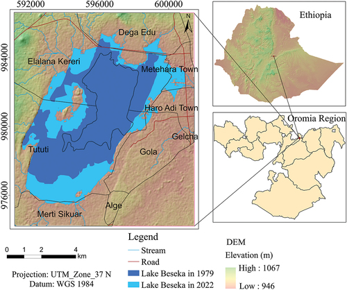
The study area is located in the northern parts of the MER, in the Oromia Regional state of East Shoa Zone in Fentale district 200 km from Addis Ababa. It is located in a recent volcano-tectonically area with a spatial extent of 591,038−601497 m N and 974,300−986706 m E covering a total area e of 129.3 km² (Figure 1). The surface area of the lake has expanded from nearly 3 to 50 km² in recent times. The area is bounded by a volcanic crater of Mount Fentale and undulating plateaus in the north and northeast directions (Dinka, 2012). The lake elevation of varies from 946 − 952 m above Mean Sea Level (MSL) with an average bathymetric depth of 6 m. The area is characterized by features of historic and recent volcanic craters and traces of fault lines (Melkamu et al., 2022). The northern central portion of the lake was the deepest and original part of the lake before it became expanded. The climate of the area is characterized by arid to semiarid climates (Mechal et al., 2022; Rango et al., 2010) and bimodal rainfall distribution patterns (Dinka, 2017b; Gichamo et al., 2022). The highest rainfall in the area occurs from July to September whereas minimal rainfall occurs in the autumn season from the end of February to April (Dinka, 2017b; Gichamo et al., 2022). The mean annual rainfall of the area is about 543.7 mm and maximum and minimum temperatures of 32.9 and 17.5°C, respectively (Gichamo et al., 2022).

Figure 1. Location map of the study area.

2.2. Data set

2.2.1. Primary and secondary water quality parameters

Primary data were obtained from field in-situ measurements of water quality parameters and satellite images. The in situ field-measured water quality parameters pH, EC, and TDS were calculated from the measured EC of the specific conductance. Secondary lake water quality parameter data were collected from the Ministry of Water and Energy (MOWE), published articles, and unpublished data sources. Primary physicochemical water quality data of the lake were collected on February 11 and 12/2023 from four sample locations. Primary data were collected using a systematic random sampling technique considering the depth of the lake and anthropogenic (Methehara influent, farm site, clothes, and car washing site) and geogenic (volcanic and hot spring) effects from the northeast and northwest portions of the lake. However, the southern and central portions of the lake were not sampled because of inaccessibility. The color of the lake varies spatially from dark in the deepest portion to yellowish-brown at the northeastern shore of the lake. The experimental analysis of the lake water sample was obtained from in-situ measurements with a HANNA Combo HI98130 pH and EC meter. Three in situ physicochemical water quality parameters, including pH and EC, were measured with the above instrument, while TDS was calculated using its relationship with the conductivity of water at 25°C ((μS/cm) and multiplication factor (0.64 for drinking water. Secondary lake water quality data were collected from published articles and unpublished data sources. Thus, secondary data were collected by considering the depth of the lake, hot spring, and anthropogenic factors, including the pumping site, Metehara town sewage, clothes, and car washing sites.

The secondary data collected (Wubet, 2007) were sampled using a systematic random sampling approach. Hence, this approach is valuable for systematically stratifying the lake into regions of similar depth, spatial gradient changes in the physical properties of the lake, directions of underground inflow of hot springs into the lake, underground outflow of water from the lake, and outflow of lake water into the Awash River. Furthermore, a systematic random sampling approach is advantageous for obtaining a small number of samples with a lesser amount of bias. Physicochemical parameters, including EC, pH, and TDS, were measured in the field using digital-portable conductivity (JENWAY 4200, UK) and pH (JENWAY 430, UK) meters (Wubet, 2007). Secondary data collected by Umer et al. (2020) were obtained during the dry season from March to April from the four corners of the lake and two samples from the central portion of the lake. This sample was duplicated to reduce bias during sampling and measurement. The samples were collected using systematic random sampling techniques by considering anthropogenic factors (influent from Metahara Town, effluent from sugarcane irrigation drainage canals, hot springs, and bathymetric depth of the lake). The pH and EC were measured in situ using a Hach HQD field case model 58258 − 00 instrument, whereas TDS was analyzed in the laboratory with APHA 2540 B, in which the total solids were dried at 103–105°C. The data collected (Tenagashaw & Tamirat, 2022) were also sampled using systematic sampling techniques that considered runoff, outflow, and groundwater inflow during the dry season. These samples were analyzed at the Abbay Basin Development Authority Water and Wastewater Laboratory (Tenagashaw & Tamirat, 2022). Generally, four primary water quality data were collected with 21 secondary water quality data by considering anthropogenic and natural factors, including pumping site, lake depth, hot spring site, and car/close washing sites, to develop equations and estimate water quality parameters. A quantitative sampling technique was used to assess the lake water quality. Hence, water quality data and surface reflectance values were expressed quantitatively. Therefore, considering the above information, the sampling method used was a systematic random sampling technique. Secondary water quality data were collected by considering the aforementioned determinant factors.

2.2.2. Satellite data

Landsat 7 ETM+ and Landsat 8 OLI/TIRS with path 168 and row 054 were downloaded from the United States Geological Survey (USGS, https://glovis.usgs.gov). The details of the data sources and their specifications are presented in (Table 1). The processed satellite image data were used to estimate the water quality of the lake by combining it with observed water quality parameter data. Field sample collection and data analysis were performed on the same day as the satellite image acquisition date to increase accuracy by reducing atmospheric and environmental influences (Batur & Maktav, 2019; Kapalanga et al., 2021; Omondi et al., 2023). Thus, cross-ponding satellite images for the primary water quality parameter data of the lake were taken on the same day as the flight of the Landsat 8 satellite. However, for secondary data, the closest cross-ponding satellite image was used.

Table 1. Wavelength ranges for Landsat ETM⁺ and Landsat 8 OLI and TIRS.

Landsat 7 ETM+		Landsat 8 OLI and TIRS		Spatial resolution (m)
Bands	Wavelength (μm)	Bands	Wavelength (μm)
1 Blue	0.45 − 0.52	2 Blue	0.45 − 0.51	30 × 30
2 Green	0.52 − 0.60	3 Green	0.53 − 0.59	30 × 30
3 Red	0.63 − 0.69	4 Red	0.64 − 0.67	30 × 30
4 NIR	0.77 − 0.90	5 NIR	0.85 − 0.88	30 × 30
5 SWIR 1	1.55 − 1.75	6 SWIR 1	1.57 − 1.65	30 × 30
7 SWIR 2	2.09 − 2.35	7 SWIR 2	2.11 − 2.29	30 × 30
6 Thermal Infrared	10.40 − 12.50	10 TIRS 1	10.6 − 11.19	Resampled 30 × 30

2.3. Methods and data analysis

Primary and secondary water quality parameters data of Lake Beseka were collected for the years 2007, 2018, 2021, and 2023. Over all methodological framework and data analysis are presented in Figure 2. The surface reflectance of the satellite images for each cross-ponding time series was extracted using those primary and secondary lake water quality parameters. To determine the statistical model, the observed water quality parameters data were used as the dependent variable whereas the surface reflectance value of each band, band ratio, and band combination were used as the independent variable (Maliki et al., 2020). For this study, the primary and secondary observed water quality parameters data were used as dependent variables, and surface reflectance of individual bands, band ratios, band combination, and water indices were used as independent variables to make linear regression and correlation.

Figure 2. The general workflow approach of the study.

2.3.1. Image processing

Satellite images were preprocessed before the surface reflectance value was generated and used for further physicochemical water quality parameters assessment. The visible and infrared portions of the electromagnetic spectrum are optical remote sensing regions that are valuable to assess water quality parameters (Avdan et al., 2019). The optical remote sensing data were radiometrically and geometrically corrected before statistical analysis was performed (Abbas et al., 2019; W. Ahmed et al., 2023; Al-Shaibah et al., 2021). Preprocessing carried out for Landsat 7 ETM+, and Landsat 8 OLI/TIRS imageries include radiometric correction (haze and noise reduction), geometric correction (by providers), layer stacking, and sub setting. Another task of pre-processing includes scan-line error correction (SLC), which is applied for the Landsat 7 ETM+ images (bands 1 to 6). The SLC was performed using the gap-fill tool in QGIS 3.24.3. On the other hand, ArcGIS 10.8 was utilized for storing, handling, evaluating the data, and layout map preparation.

2.3.1.1. Geometric correction

Geometrically corrected Landsat series C2L2 images are downloaded from the USGS website and their spatial location was cross-checked for each band and scene at the level of pixel size.

2.3.1.2. Radiometric correction

In radiometric correction, the digital number or pixel value is converted into reflectance value by using Landsat series C2L2 metadata rescaling factors as given by Al-Shaibah et al. (2021).

(1) ${\mathrm{L}}_{\mathit{\lambda }}=\mathrm{ML}\times \mathrm{Qcal}+\mathrm{AL}$(1)

where L_λ top of atmospheric reflectance, ML is the reflectance multiplicative factors, Qcal is the DN value, and AL is the additive factor of each band which is found in the metadata file of each scene.

2.3.1.3. Atmospheric correction

The electromagnetic radiation interacts with the atmosphere twice, once when it radiates to the earth’s surface and again it is reflected toward the sensors. During its propagation, electromagnetic radiation can be affected by atmospheric effects, which need atmospheric corrections. After radiometric correction was done, atmospheric correction could be applied to remove the atmospheric factors that affect the movement of surface reflection and to transform the radiometric value into surface reflectance (Al-Shaibah et al., 2021).

2.4. Water body extraction

The water body of the lake was extracted using different water indices including Normalized Difference Water Index (NDMI), Modified Normalized Difference Water Index (MNDWI), and Automatic Water Extraction Index (AWEI) from Landsat 7 ETM⁺ and Landsat 8 OLI images of 2007, 2018, 2021, and 2023. Thus, extracted water body was used to mask satellite images in which surface reflectance point data were generated. The Normalized Difference Water Index (NDMI) was used to extract water bodies from non-water bodies (Melkamu et al., 2022). It uses a green band to increase surface water reflectance and minimize the reflectance of the NIR band by water surface and to get the advantage of higher reflectance of NIR by soil and vegetation classified as per McFeeters (1996).

(2) $\mathrm{NDWI}=\frac{\mathrm{Green}-\mathrm{NIR}}{\mathrm{Green}+\mathrm{NIR}}$(2)

where NDWI is the normalized difference water index and NIR is the spectral value of the near-infrared band. The modified normalized difference water index (MNDWI) method as shown (eq.3) can be used to separate the effect of noise of constructed built-up features, which is not answered by NDWI question features as given by Xu (2006).

(3) $\mathrm{MNDWI}=\frac{\mathrm{Green}-\mathrm{SWIR}1}{\mathrm{Green}+\mathrm{SWIR}1}$(3)

where SWIR1 is short wave infrared 1 band.

Furthermore, the Automatic Water Extraction Index (AWEI) developed by Feyisa et al. (2014) is used to diminish the effect of the presence or absence of cloud or dark surfaces on earth features (eq.4 & eq.5).

(4) $\mathrm{AWEInsh}=4\times \left(\mathrm{Green}-\mathrm{SWIR}1\right)-\left(0.25\times \mathrm{NIR}+2.75\times \mathrm{SWIR}2\right)$(4)

(5) $\mathrm{AWEIsh}=\mathrm{Blue}+2.5\times \mathrm{Green}-1.5\mathit{\hspace{0.17em}}\times \left(\mathrm{NIR}+\mathrm{SWIR}1\right)-0.25\times \mathrm{SWIR}2)$(5)

where AWEInsh is the automatic water extraction index for areas where the shadow is not a problem and AWEIsh is where shadow and dark surface are problems on the required area, SWIR1 and SWIR2 are short wave infrared region 1 and 2 bands, respectively.

2.5. Surface reflectance extraction

For water quality parameters estimations, 10 scenes on path 168 and row 054 were used to calculate the surface reflectance data of the lake. Three scenes for the year 2007, one scene for the year 2018, five scenes for the year 2021, and one scene for the year 2023 cloud-free Landsat images are selected and averaged to get single scenes for each year individual bands using ArcGIS raster calculating tools. The cross-ponding surface reflectance value for lake water quality parameters (EC, TDS, and pH) of the individual bands was extracted using ArcGIS to extract multiple values to points tools within the same location. Thus, the correlation was made between observed data and spectral data (bands, band ratio, and indices) (W. Ahmed et al., 2023; Jakovljevic et al., 2024; Omondi et al., 2023).

2.6. Data analysis

For statistical analysis, surface reflectance at the pixel level was extracted using in‐situ water quality parameters point data using the extract multi-values to points ArcGIS tool (Hossain et al., 2021). In-situ Lake Water Quality Parameters (LWQPs) and satellite image surface reflectance data sets were used to assess water quality (Mishra et al., 2021). The correlation between satellite image surface reflectance and water quality data including pH, EC, and TDS can estimate surface water quality change (Japitana & Burce, 2019). LWQPs data are correlated to each other and with various band ratios, band combinations, and individual bands derived from Landsat imagery (Al-Shaibah et al., 2021).

In the present study, the surface reflectance of Landsat 7 ETM+ for the year 2007 and Landsat 8 OLI for the years 2018, 2021, and 2023 data were extracted using the extract multi-values to points ArcGIS tool using in-situ primary and secondary LWQPS data at a pixel level. Statistical analysis was conducted using those extracted surface reflectance values of individual bands, band combinations, band ratios, and water indices with primary and secondary in‐situ LWQPs data to find out highly correlated data. The band operations were done for optical satellite image surface reflectance data of 91 band operations (Table 2). Input data for six individual bands, two water indices, and 25 band combination, and 58 band ratios were used to find out highly correlated operations for each water quality parameter. The plot of in-situ LWQPs data and satellite image reflectance data were used to estimate their relationship.

Table 2. Band operations that are used for regression and correlation analysis with in-situ water quality parameters.

Individual bands	Band combinations	Band ratios	Water indices
B2, B3, B4, B5, B6, B7	B2+B3, B2+B4, B2+B5, B2+B6, B2+B7, B3+B4, B3+B5, B3+B6, B3+B7, B4+B5, B4+B6, B4+B7, B5+B6, B5+B7, B6+B7, B2+B3+B4, B2+B3+B5, B2+B3+B6, B2+B3+B7, B3+B4+B5, B3+B4+B6, B3+B4+B7, B4+B5+B6, B4+B5+B7, B5+B6+B7	B2/B3, B2/B4, B2/B5, B2/B6, B2/B7, B3/B2, B3/B4, B3/B5, B3/B6, B3/B7, B4/B2, B4/B3, B4/B5, B4/B6, B4/B7, B5/B2, B5/B3, B5/B4, B5/B6, B5/B7, B6/B2, B6/B3, B6/B4, B6/B5, B6/B7, B7/B2, B7/B3, B7/B4, B7/B5, B7/B6, B2/B3+B4, B2/B3+B5, B2/B3+B6, B2/B3+B7, B3/B2+B4, B3/B2+B5, B3/B2+B6, B3/B2+B7, B4/B2+B3, B4/B2+B5, B4/B2+B6, B4/B2+B7, B4/B3+B5, B4/B3+B6, B4/B3+B7, B4/B5+B6, B4/B5+B7, B4/B6+B7, B5/B2+B3, B5/B2+B4, B5/B2+B6, B5/B2+B7, B5/B3+B4, B5/B3+B6, B5/B3+B7, B5/B4+B6, B5/B4+B7, B5/B6+B7	NDWI=B3−B5/B3+B5 MNDWI=B3−B6/B3+B6

where B2, B3, B4, B5, B6, and B7 are band 2/blue, band 3/green, band 4/red, band 5/near infrared, band 6/short wave infrared1, and band 7/short wave Infrared 2, respectively.

2.6.1. Correlation

In bivariate distribution, two variables are integrated to find out their relationship in which the existence of one variable affects the other variable (Sarma, 2009). The correlation determined the strength of the relationship between variables while regression analysis was used to develop equations based on their relationship (Abdelmalik, 2018). Therefore, the Pearson coefficient correlation was used to test the relationship between in‐situ LWQPs data and reflectance (W. Ahmed et al., 2023; Al-Shaibah et al., 2021; Maliki et al., 2020; Mishra et al., 2021). The coefficient of correlation is the most commonly used to summarize bivariate comparisons. If σx and σy are the standard deviations for two variables, their correlation coefficients are shown (eq. 6).

(6) $\mathrm{r}\left(\mathrm{X},\mathrm{Y}\right)=\mathit{\hspace{0.17em}}\frac{\mathrm{Cov}\left(\mathrm{X},\mathrm{Y}\right)}{{\mathit{\sigma }}_{\mathrm{X}\times }{\mathit{\sigma }}_{\mathrm{Y}}}$(6)

where r (X, Y) varies continuously from − 1 to 1; If it is 1, perfect direct linear correlation, if it is 0, no linear correlation, and if it is − 1, perfectly inverse correlation.

2.6.2. Regression

Scholars use different types of regression techniques based on their objectives and data availability. A linear regression technique is used to determine the relationship between two variables which helps to predict one variable (Sarma, 2009). Statistical analysis of TDS and temperature can be done to determine a regression model either linear or nonlinear regression models with Landsat image reflectance (Cruz-Retana et al., 2023; Li et al., 2021). The multiple linear regression method was analyzed with R Studio to accomplish the relationship between water quality parameters and satellite reflectance data (Pizani et al., 2020; Omondi et al., 2023). Thus, scholars including (Abdelmalik, 2018; W. Ahmed et al., 2023; Li et al., 2021; Yang et al., 2022) applied regression and correlation analysis between observed water quality parameters of pH, TDS, and EC with surface reflectance of the satellite image.

2.6.3. Equation development

Statistical analysis of surface water quality parameters including pH, TDS, and EC can be determined by linear regression models with Landsat image surface reflectance. Hence, in-situ LWQPs and satellite image surface reflectance values are correlated and regressed to develop a model to determine surface water quality. An empirical model developed from Landsat images and water quality data accurately estimates water quality parameters (Al-Shaibah et al., 2021; Japitana & Burce, 2019). For this study, the linear regressions were analyzed with R Studio 3.6.3 and Microsoft Excel 2016.

The correlation between surface reflectance value of individual bands, band combination, band ratios, and water indices were determined. After linear regression analysis was performed, some highly correlated operations were selected based on Pearson the coefficient of correlation value for validation to estimate water quality change (Akbar et al., 2014; Al-Shaibah et al., 2021; Jakovljevic et al., 2024). Hence, regression analysis was undertaken to find out the best-fitted model of surface reflectance value with in-situ measured water quality parameters. According to Al-Shaibah et al. (2021), both in-situ water quality parameters and estimated results exhibited the same trends. As a result, from 91 band operations, some highly correlated operations were selected to validate the developed linear regression equations.

2.6.4. Model validation

Training samples for the model were used to develop an equation that determines the relation between in-situ and surface reflectance satellite image data (Al-Shaibah et al., 2021). The field datasets were used to check the accuracy of calculated water quality. Microsoft Excel software was utilized to perform the statistical analysis for training (75%) and validating (25%) and used to compare the performance of the developed question in the training phase (Mohamed et al., 2022). Hence, for this study, R Studio 3.6.3 and Microsoft Excel 2016 software were used to make the correlation. Scholars use different model-validating techniques to validate the developed empirical equations. Jakovljevic et al. (2024); Li et al. (2021); Omondi et al. (2023) uses the coefficient of correlation, Al-Shaibah et al. (2021) use p-value, and Japitana and Burce (2019) use a t-test to validate their models. Thus, the calibration and validation would be done based on the Root Mean Square Error question (RMSE) (eq.7). For this analysis, 25 in-situ data were collected for the years 2007, 2018, 2021, and 2023 for calibration and validation. From the total 25 data, 75% (19) data were selected for calibration and 25% (6) data were used for validation. Thus, the selected 6 data were used to validate the selected linear regression equation based on RMSE, p-value, and R² to select the best equation that was used to predict each water quality parameter of Lake Beseka. Finally, the selected and validated LWQPs equation was applied to estimate and map the lake water quality expanding and diluting Lake Beseka using the geostatistical tool with the kriging method. Hence, it performs 10% better as compared to the inverse distance weighted method as suggested by Omondi et al. (2023).

(7) $\mathrm{RMSE}=\sqrt{\sum _{\mathrm{i}=1}^{\mathrm{n}}\frac{{\left({\mathrm{x}}_{\mathrm{i}}-{\mathrm{y}}_{\mathrm{i}}\right)}^2}{\mathrm{n}}\mathit{\hspace{0.17em}}}$(7)

where x_i is the in‐situ water quality parameter, yi is the estimated water quality parameter from the developed equation, and n is the number of observations.

3. Results

The optical Landsat satellite image is applicable to estimate and monitor surface water quality parameters. Linear regressions equations that were developed from Landsat 7 ETM+ and Landsat 8 OLI surface reflectance data and observed water quality parameters for the years 2007, 2018, 2021, and 2023 indicates in (Table 3). The analysis was done to estimate the spatiotemporal water quality parameter change of Lake Beseka. The relatively higher regression and correlation analysis results for observed water quality data and surface reflectance value of a given band operations were indicated (Table 4). The higher Pearson coefficient of correlation for calibration and validation analysis for each parameter were used to estimate water quality parameters of the lake.

Table 3. Observed water quality parameters and surface reflectance data for the years 2007, 2018, 2021, and 2023.

S No	pH	TDS (mg/l)	EC (μS/cm)	Band 2	Band 3	Band 4	Band 5	Band 6	Band 7	Scource
W 1	9.4	4160	6960	0.066	0.041	0.029	0.019	0.010	0.007	Wubet (2007)
W 2	9.52	4220	7060	0.066	0.042	0.028	0.022	0.010	0.009
W 3	9.52	4150	6910	0.066	0.041	0.030	0.022	0.010	0.005
W 4	9.64	3600	6660	0.075	0.050	0.039	0.032	0.021	0.015
W 5	9.52	4120	6880	0.070	0.047	0.035	0.030	0.014	0.007
W 6	8.36	1020	1710	0.086	0.065	0.054	0.060	0.052	0.031
W 7	9.42	2880	4790	0.078	0.053	0.044	0.038	0.025	0.016
B 1	7.33	831.17	1663	0.103	0.083	0.075	0.058	0.036	0.026	Umer et al. (2020)
B 2	7.33	831.17	1663	0.112	0.101	0.098	0.117	0.076	0.056
B 3	7.97	840.13	1615	0.105	0.090	0.085	0.095	0.059	0.041
B 4	8.7	858.83	1719	0.098	0.082	0.073	0.074	0.035	0.022
B 5	8.1	867.67	1613	0.110	0.094	0.089	0.088	0.054	0.039
B 6	7.81	874.5	1563	0.114	0.097	0.091	0.081	0.056	0.042
S 1	9.42	1880	2950	0.089	0.075	0.068	0.039	0.020	0.075	Tenagashaw and Tamirat (2022)
S 2	8.92	1851	2894	0.089	0.076	0.069	0.039	0.020	0.078
S 3	9.33	1793	2813	0.089	0.077	0.069	0.041	0.019	0.072
S 4	9.42	1770	2783	0.088	0.074	0.066	0.036	0.017	0.059
S 5	9.76	1783	2790	0.086	0.071	0.061	0.033	0.015	0.052
S 6	8.98	1885	2975	0.085	0.070	0.060	0.032	0.014	0.052
S 7	9.58	2436	3746	0.079	0.058	0.047	0.033	0.018	0.068
S 8	9.12	1830	2870	0.087	0.073	0.065	0.032	0.014	0.051
L 1	8.99	1132.8	1770	0.0661	0.0501	0.0391	0.0236	0.0141	0.0110	In-situ
L 2	8.92	1574.4	2460	0.0646	0.0475	0.0355	0.0207	0.0119	0.0094
L 3	8.93	1830	2860	0.0645	0.0473	0.0354	0.0213	0.0126	0.0097
L 4	8.82	1715.2	2680	0.0671	0.0520	0.0408	0.0283	0.0190	0.0163

Table 4. Dry season linear regression and correlation analysis between observed water quality parameters and surface reflectance data.

WQPs	Band operations	Calibration			Validation
		Equation	R^2	r	R^2	RMSE	r	P-value
pH	B5	pH = −22.84×(B5) +9.91	0.58	−0.76	0.83	0.34	0.91	0.01
	B6	pH = −32.02×(B6) +9.74	0.62	−0.79	0.89	0.25	0.94	0.005
	B2+B6	pH = −17.31×(B2+B6) +10.83	0.60	−0.78	0.83	0.40	0.89	0.02
	B3+B6	pH = −16.32×(B3+B6) +10.42	0.58	−0.76	0.86	0.26	93	0.007
	B5+B6	pH = −13.63×(B5+B6) +9.86	0.61	−0.78	0.86	0.30	0.93	0.008
	B4+B5+B6	pH = −9.23×(B4+B5+B6) +10.08	0.58	−0.76	0.86	0.28	0.92	0.008
EC	B2/B3	EC = 11083.89×(B2/B3) −11144.58	0.74	0.86	0.91	548	0.95	0.003
	B2/B4	EC = 4639.68×(B2/B4) −4021.07	0.69	0.83	0.86	666	0.93	0.007
	B3/B2	EC = −19570.50×(B3/B2) +18507.86	0.69	−0.83	0.86	692	0.93	0.008
	B2/(B3+B4)	EC = 14421.69×B2/(B3+B4) −6961.74	0.71	0.84	0.88	619	0.94	0.005
TDS	B2/B3	TDS = 6416.63×(B2/B3) −6377.45	0.72	0.85	0.90	367	0.95	0.004
	B2/B4	TDS = 2726.1×(B2/B4) −2317.8	0.69	0.83	0.87	433	0.93	0.007
	B3/B2	TDS = −11333.47×(B3/B2) +10791.74	0.67	−0.81	0.87	424	0.93	0.007
	B2/(B3+B4)	TDS = 8426.78×B2/(B3+B4) −4011.92	0.62	0.84	0.88	400	0.94	0.006

3.1. Powers of hydrogen (pH)

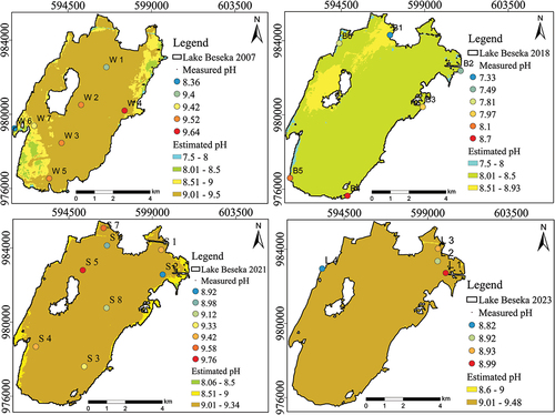
Direct estimation of surface water pH from satellite images is impractical. However, it can be estimated indirectly from a linear regression equation that developed from field/laboratory measurement and surface reflectance value of satellite image data. Thus, optical satellite images are applied to estimate the pH value of the surface water bodies. The higher Pearson coefficient of correlation and R² between observed pH and surface reflectance value of optical satellite image occurred in band combinations and individual bands of band 5, band 6, band 2+band 6, band 5+band 6, band 3+band 6, and band 4+band 5+band 6 (Figure 3). The Pearson coefficient of correlation for all selected band operations was negative which indicates the inverse relationship between the observed pH and surface reflectance value of optical Landsat images. Even if, the statistically analyzed results for all selected band operations were close to each other, the highest Pearson coefficient of correlation and R² existed in band 6 with the values of − 0.79 and 0.62, respectively (Table 4). Similarly, the validation analysis for band 6 also had high R² and Pearson coefficient of correlation and low RMSE and p-values of 0.89, 0.94, 0.25, and 0.005, respectively (Figure 4). Hence, the spatiotemporal pH map of Lake Beseka was estimated from a linear regression equation that developed from the observed pH and surface reflectance of band 6 (SWIR 1). The estimated pH varied from 7.5 − 9.5, 7.5 − 8.93, 8.06 − 9.34, and 8.6 − 9.48 for the years 2007, 2018, 2021, and 2023, respectively (Figure 5). The highest estimated pH value was found in the central portion of the lake and the lowest was found in the southwestern and northeastern shore of the lake. However, the estimated pH value for the year 2018 was lower than other years.

Figure 3. Linear regression and correlation analysis for pH.

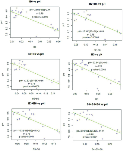
Figure 4. Validation analysis between observed and estimated pH.

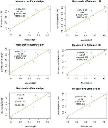
Figure 5. The estimated spatiotemporal map of pH.

3.2. Electrical conductivity

The electrical conductivity of the surface water bodies also cannot be directly estimated from satellite images. It can be determined from a linear regression equation that developed from the surface reflectance of satellite images and observed EC data. For this study, a linear regression equation was developed from the surface reflectance value of Landsat 7 ETM⁺ and Landsat 8 OLI images and observed EC data for the years 2007, 2018, 2021, and 2023. The higher Pearson coefficient of correlation and R² occurred in the band ratios of band 2/band 3, band 2/band 4, band 2/(band 3 + band 4), and band 3/band 2 (Figure 6). However, the highest Pearson coefficient of correlation and R² for calibration analysis existed in band 2/band 3 with values of 0.86 and 0.74 (Table 4), respectively. In addition, the best-fitted linear regression equation from the validation analysis was found in the band 2/band 3 band ratio with Pearson coefficient of correlation, R², p-value, and RMSE values of 0.95, 0.91, 0.003, and 548, respectively. Therefore, the estimated EC of the lake was determined using a linear regression equation of the band2/band3 band ratio (Table 5). Therefore, the dry season spatiotemporal EC map of Lake Beseka was estimated from the best-fitted linear regression equation developed from observed EC data and optical surface reflectance Landsat images of band 2/band 3 band ratio (Figure 7). The estimated EC of the lake varied from 500 − 7798 μS/cm, 1000 − 3000 μS/cm, 500 − 4131 μS/cm, and 500 − 5232 μS/cm for the years 2007, 2018, 2021, and 2023 (Figure 8), respectively. The estimated EC concentration was high for the years 2007 and 2023 and increased from the shores to the central portion of the lake. However, the concentration for the years 2018 and 2021 was relatively lower than others. Spatially, some anomalies occurred in the western parts of the island for the year 2018 and northern shore for the years 2018 and 2021.

Figure 6. Linear regression and correlation analysis for EC.

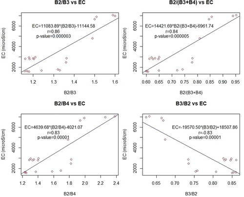
Figure 7. Validation analysis between observed and estimated EC.

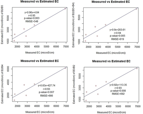
Figure 8. The estimated spatiotemporal map of EC.

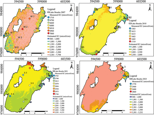
Table 5. Selected linear regression equation to estimate dry season water quality parameters.

WQPs	Band operations	Calibration			Validation
		Equation	R^2	r	R^2	RMSE	r	P-value
pH	B6	pH = −32.02×(B6) +9.74	0.62	−0.79	0.89	0.25	0.94	0.005
EC	B2/B3	EC = 11083.89×(B2/B3) −11144.58	0.74	0.86	0.91	548	0.95	0.003
TDS	B2/B3	TDS = 6416.63×(B2/B3) −6377.45	0.72	0.85	0.90	367	0.95	0.004

3.3. Total dissolved solids

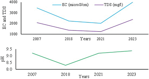
Similar to the EC statistical data analysis, the linear regression equation for TDS was high in-band ratios rather than individual bands, band combinations, and water indices (Table 4). Those band ratios were band 2/band 3, band 2/band 4, band 3/band 2, and band 2/(band 3 + band 4) (Figure 9). The Pearson coefficient of correlations for all selected band operations was found between 71 − 85%. However, the highest Pearson coefficient of correlation for dry season calibration analysis existed in the band ratio of band2/band3 similar to EC data analysis. Thus, the water spectrum is an obvious reflection in the band 3 and the absorption continues to increase after the band 4. In addition, the highest Pearson coefficient of correlation and R² and the lowest RMSE and p-value for the validation analysis data occurred in the band ratio of band2/band3 with values of 0.95, 0.90, 367, and 0.004, respectively (Table 4). The graph of linear regression for both calibration and validation analysis were indicated in (Figures 9 and 10), respectively. The estimated TDS value of the lake varies from 500 − 4589 mg/l, 615 − 1931 mg/l, 600 − 2466 mg/l, and 500 − 3000 mg/l in 2007, 2018, 2021, and 2023, respectively (Figure 11). The lowest estimated TDS concentration existed in the northeastern, southern, and southwestern shores of the lake. The concentration increased from the shore to the central portion of the lake. However, the estimated TDS for the years 2018 and 2021 were lower than the years 2007 and 2023 in a similar pattern with EC concentration. The estimated mean pH was 8.3 which occurred for the year 2018 (Figure 12). However, the mean estimated EC and TDS of the lake was lower in 2021 with values of 2022 μS/cm and 1245 mg/l, respectively. The relatively high estimated concentration of the lake for all water quality parameters occurred in 2007 and 2023.

Figure 9. Linear regression and correlation analysis for TDS.

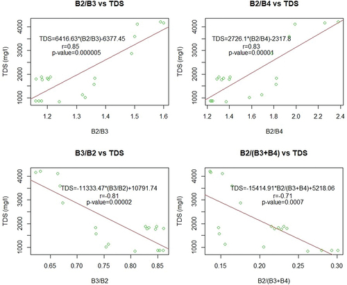
Figure 10. Validation analysis between measured and estimated TDS.

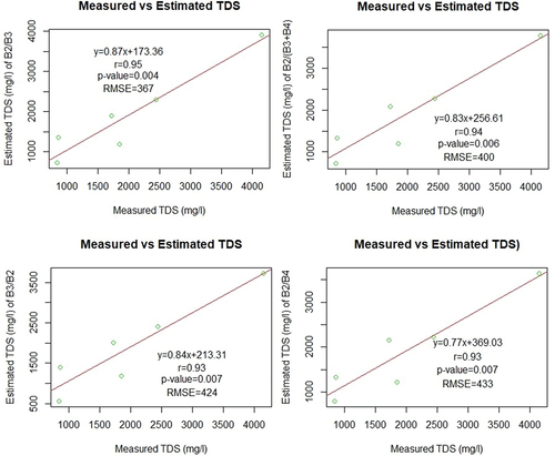
Figure 11. The estimated spatiotemporal map of TDS.

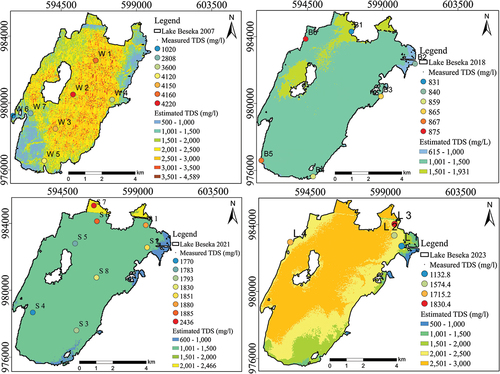
Figure 12. The estimated mean water quality parameters change.

4. Discussion

Several satellite images could be utilized to evaluate the quality of the water. Nonetheless, Landsat images have been used extensively due to their relatively low cost, temporal coverage, and spatial resolution (Omeka & Egbueri, 2023; Omeka et al., 2024). The surface reflectance of the optical image was obtained from Landsat 7 ETM⁺ and Landsat 8 OLI. Those optical individual bands, band combinations, band ratios, and water indices were correlated and regressed with observed water quality parameters. The best-fitted linear regression equation for EC and TDS existed in the band ratios of blue and green wavelengths ranging whereas the pH was estimated from the linear regression equation of band 6. The trends of in-situ and estimated water quality parameters exhibited similarly (Al-Shaibah et al., 2021). Li et al. (2021) conducted research to assess the extent and pattern with different water indices and got a relatively high correlation analysis on normalized water indices for TDS, pH, and salinity. Nevertheless, it should be noted that there is a spatial resolution difference between sensors i.e., 30 m for Landsat 7 ETM+ and Landsat 8 and other satellite data products. Besides that, Landsat 8 image was retrieved using the blue, green, and SWIR1 bands to estimate TDS and pH effectively (W. Ahmed et al., 2023).

4.1. pH

The best-fitted linear regression equation for pH occurred in the SWIR1 wavelength range of the Landsat image. The R² and Pearson correlation coefficients for pH calibration and validation were high in SWIR. Further, the surface reflectance of SWIR1 and the observed pH of the lake have high negative correlations, with the observed pH decreasing as the surface reflectance value of SWIR1 increased (Figure 3). The RMSE and p-value for the measured and observed pH were relatively lower than band operation SWIR1. According to Abbas et al. (2019), Landsat 5 TM at the SWIR1 region was used to estimate pH concentration from a best-fitted linear regression analysis. In contrast to that noted by W. Ahmed et al. (2023), the estimate of pH from Landsat 8 image blue, green, and SWIR1 bands (W. Ahmed et al., 2023). The present results are line with the findings of Li et al. (2021) who fund a pH has a negative coefficient of correlation while TDS and salinity have a positive correlation. Pereira et al. (2020) observed that pH was estimated using the Google Earth engine and linear regression analysis from different water indices and individual bands.

The estimated spatiotemporal pH map of Lake Beseka shows some variation for the given years. The major portion of the lake for the years 2007, 2021, and 2023 has a pH value of 9−9.5 and the lowest value occurred in the southwestern and northeastern shores of the lake for the years 2007, 2018, and 2021. Overall, the pH on the southwestern shore of the lake was lower than the central portions. This was due to the discharge of hot springs that have a relatively low pH concentration to the lake (Goerner et al., 2009). However, the major portion of the lake for the year 2018 contains an estimated pH between 8.01 and 8.5. The observed pH for the year 2018 also had a lower concentration as compared with the other years. However, relatively high estimated pH of the lake was indicated near the west and north of the island.

4.2. Electrical conductivity

The EC of the lake was estimated from the blue/green band ratio of the Landsat image’s surface reflectance. Thus, the best-fitted linear regression equation occurred in the band2/band3 band ratio (Figure 6). A strong positive correlation existed in the band ratios rather than individual bands hence, band ratios eliminate the atmospheric influences (Mohamed et al., 2022). The estimated EC was determined from a linear regression equation with a band ratio of green to red bands (Abbas et al., 2019). Thus, water has high reflectance at blue-green bands and absorbs radiation at near-infrared and beyond portion of the electromagnetic spectrum (Jakovljevic et al., 2024).

Furthermore, the Pearson correlation coefficient between the mean surface reflectance of Landsat 8 optical bands and measured EC was negative (Mishra et al., 2021). However, for this study, the blue and red band ratios have a higher positive correlation than the green and red band ratios. According to Mohamed et al. (2022), a very strong positive correlation occurred between observed EC and Landsat band ratios (B2/B4, B2/B3, B3/B4, B4/B7, and B6/B5) with R² >0.80 and the validation analysis was higher in band ratio of B3/B4. The reason is that EC is sensitive to the visible electromagnetic spectrum (Avdan et al., 2019). The R² and Pearson correlation coefficients for EC data calibration and validation were higher in the blue/green band ratio with a positive correlation. The RMSE and p-value of the validation analysis were lower in the blue/green band ratio. Therefore, this best-fitted linear regression equation estimated the spatiotemporal EC map.

The highest estimated EC concentration of the lake occurred in 2007 and has decreased since 2018 and 2021, with a later increment for 2023. In addition, the spatial distribution of the estimated EC increased from the shores to the central portion of the lake for the given years. The EC concentration of the hot spring and Lake Beseka varies from 4000 − 5000 μS/cm and 6200 − 15000 μS/cm, respectively (Dinka et al., 2015) that indicates the EC of the hot spring lower than lake water and the hot spring dilutes the lake water. According to Belay (2009), the lake water EC after the 1980s shows a trivial increment compared to the 1960s to 1980, and the dilution trends might be related to diminishing water inflow or increasing evaporation rate. Therefore, such conditions might also cause a recent relative increment after 2018. The lowest concentration was found on the lake’s northeastern shore, followed by the lake’s southern shore for all years. The EC concentration of the lake for 2018 and 2021 was relatively lower than for 2007 and 2023. However, the EC concentration in 2018 indicates some anomalies in the western and northern sides apart from the main island, even if a higher concentration occurred at the lake’s north shore for the year 2021.

4.3. Total dissolved solids

The TDS value of the lake was also estimated from the band ratio of blue and green bands. Hence, the best-fitted linear regression equation was found in the blue/green band ratio. According to Maliki et al. (2020), TDS concentration can be estimated using Landsat optical images of the salinity index from blue and green bands. In contrast to that noted by Ferdous et al. (2019), estimate TDS with 83.6% accuracy from a regression equation that developed from blue, green, and red bands. Other earlier authors Abbas et al. (2019), got a higher coefficient of correction for TDS estimation from the band ratio of NIR and SWIR1. The R² and Pearson coefficient of correlation for training TDS data were 0.72 and 0.85, respectively (Table 4). Thus, the surface reflectance of the blue/green band ratio and measured TDS had a positive correlation. However, Mishra et al. (2021), surprisingly found a strong negative correlation between the mean surface reflectance of Landsat 8 optical bands and measured TDS. The validation analysis for measured and estimated TDS data were 0.90, 0.95, 367, and 0.004 for the r², Pearson correlation coefficient, RMSE, and p-value, respectively.

The estimated spatiotemporal TDS map of the lake has the same pattern as the EC map. The highest estimated TDS concentration was found for the year 2007 with value ranged from 3000 to 4589 mg/l as compared with other years. The major portion of the lake for the years 2018 and 2021 had TDS concentration ranged from 1000 to 1500 mg/l even though the western parts of the island and the northern shore of the lake have some anomalies. Similarly, the observed TDS for the years 2018 and 2021 also decreased as compared with the years 2007 and 2023. But for the year 2023, the most central portion of the lake was containing 2500−3000 mg/l. The lowest TDS concentration for all estimated years was found in the northeastern and south of the southwestern shore of the lake and the highest was found in the central portion that grouped under brackish water. Thus, the hot spring water in southwestern and western shores of the lake had low pH and EC concentration (Belay, 2009; Goerner et al., 2009). In addition, the central portion of the lake was characterized by high EC concentration at the maximum bathymetric depth and old ruminant saline water (Belay, 2009). According to Dinka et al. (2015), the lake was categorized under brackish water with TDS value ranged from 1000 to 10,000 mg/l. The submerged saline spring in the southwestern portion of the lake discharges 500 l/s (Kebede & Zewdu, 2019) that cause water quality variation. These results are supported by the earlier findings in the lake by Belay (2009), and Dinka (2012), justified the higher concentration of the lake due to the high evaporation rate of the lake.

Among various driving factors of spatiotemporal variation of Lake Beseka, most researchers have noticed as exercising water quality variation of Lake Beseka is due to the high evaporation rate on the lake due to its arid to semiarid climate of the area and water-level rise (Belay, 2009; Dinka et al., 2015; Kebede & Zewdu, 2019). A few studies have also distinguished groundwater influx into the lake and volcano-tectonic processes related to uplift and subsidence (Dinka, 2020; Goerner et al., 2009; Jin et al., 2021; Kebede & Zewdu, 2019). Gichamo et al. (2022) and Jin et al. (2021) conducted research to assess the irrigation water inflow from surrounding sugarcane plantation and their impact in the Awash River. The spatial variation of Lake Beseka is due to submerged saline spring in the southwestern parts of 500 l/s discharge (Kebede & Zewdu, 2019); bathymetric depth variation, and old remnant saline water at the deepest portion of the lake (Belay, 2009; Goerner et al., 2009); geology variation and recent volcanic eruption at northwestern portion of the lake (Kebede & Zewdu, 2019). In addition, to improve the water quality deterioration of the lake, the government dilutes the lake by pumping Awash River into the lake and discharging lake water to Awash River. However, in the rainy season, the lake water is highly diluted due to high runoff inflow to the lake from irrigation water and rainfall.

4.4. Limitations and recommendations

Data from remote sensing are useful for examining the temporal and geographic fluctuations of water quality parameters. Nevertheless, many significant limitations must be considered before using this method. Models created from remote sensing data may only be utilized when clouds are absent and require sufficient calibration and validation through in-situ measurements. This aids in creating a more precise empirical model for the scientific community on a regional basis. Additionally, the accuracy of the model used to predict the spatiotemporal water quality dynamics of various waterbodies is increased using ground-based sensors. Water quality assessment using remotely sensed data may be limited by the geographical, temporal, and spectral resolution constraints of many optical sensors on the market today. Water discharge and the vertical distribution of water quality indicators in waterbodies are essential factors that are difficult to assess directly using optical sensors. Therefore, it is highly recommended that local authorities and policy-makers focus on water quality and water treatment for harness removal may be required in Lake Beseka.

5. Conclusion

In recent years, anthropogenic activities have resulted in a number of processes involving human-nature interaction that have drastically damaged the quality of the water. Remote sensing data and statistical analysis in conjunction with traditional in-situ sampling are the most effective, cheaper, and more reliable tools for monitoring water quality parameters in various waterbodies such as lakes, and rivers, etc. This study was mainly focused on mapping physiochemical water quality of the expanding and diluting Lake Beseka using remote sensing and observed data. The best-fitted linear regression equation for EC and TDS occurred in a band ratio of blue to green (B2/B3) with Pearson coefficient correlation of 0.86 and 0.85 and r² of 0.74 and 0.72, respectively. The estimated EC and TDS concentration varies spatiotemporally and the higher EC and TDS existed in 2007 and 2023 that cover the dominant portion of the lake from 3500 − 7000 μS/cm and 2500 − 3000 mg/l, respectively. Moreover, the lower concentration existed in the northeastern, southwestern, and southern shores of the lake and increased from the shores to the central portion of the lake. This is due to the spatiotemporal variation of the lake, and the central portion of the lake was grouped under brackish water. Similarly, the higher concentration of pH occurred in the central portion of the lake and decreased towards the shores. Physiochemical water quality in the lakes declined between 2007 and 2021 but began to increase again in 2023. The hot springs, groundwater discharge, evaporation, seasonal variation, human, and geological influences are the main causes of the spatiotemporal variations observed in the lake’s water quality indicators. The information and the knowledge gained from the outcomes of the present study would assist local authorities and government agencies accurately identifying the water quality in the lake.

Acknowledgments

We are thankful to the School of Earth Sciences, College of Natural and Computational Sciences, Addis Ababa University for providing all kinds of necessary facilities, and support during the present study. The authors are thankful to the Ethiopian Ministry of Water and Energy for providing water quality data. Our honorable thanks extend to Mr. Abdi Umer, Mr. Hussien, and Mr. Elias Kebede who provided data and information about the area, and Mr. Tadesse Demssie for his continuous advice and comments from the beginning to the end of the study. We also wish to thank the two anonymous reviewers for their insightful suggestions and careful reading of the manuscript.

Disclosure statement

No potential conflict of interest was reported by the author(s).

Data availability statement

All data sets are available on request from the first author (Workie). The data are not publicly available because they contain information that could compromise the privacy of research participants.

References

- Abbas, R. M., Rasib, B. A., Ahmad, B. B., Musa, B. T., Abbas, R. T., & Dutsenwai, S. H. (2019). Landsat data to estimate a model of water quality parameters in Tigris and Euphrates Rivers-Iraq. International Journal of Advanced and Applied Sciences, 6(5), 50–58.
- Abdelmalik, K. W. (2018). Role of statistical remote sensing for inland water quality parameters prediction. The Egyptian Journal of Remote Sensing and Space Sciences, 21(2), 193–200. https://doi.org/10.1016/j.ejrs.2016.12.002
- Agbasi, J. C., Egbueri, J. C., Ayejoto, D. A., Unigwe, C. O., Omeka, M. E., Nwazelibe, V. E., Ighalo, J. O., Pande, C. B., & Fakoya, A. A. (2023). The Impact of Seasonal Changes on the Trends of Physicochemical, Heavy Metal and Microbial Loads in Water Resources of Southeastern Nigeria: A Critical Review. In J. C. Egbueri, J. O. Ighalo, & C. B. Pande (Eds.), Climate Change Impacts on Nigeria. Springer Climate, Springer. https://doi.org/10.1007/978-3-031-21007-5_25
- Ahmed, W., Mohammed, S., El-Shazly, A., & Morsy, S. (2023). Tigris River water surface quality monitoring using remote sensing data and GIS techniques. The Egyptian Journal of Remote Sensing and Space Sciences, 26(3), 816–825. https://doi.org/10.1016/j.ejrs.2023.09.001
- Ahmed, M., Mumtaz, R., Anwar, Z., Shaukat, A., Arif, O., & Shafait, F. (2022). A multi-step approach for optically active and inactive water quality parameter estimation using deep learning and remote sensing. Water, 14(2112), 1–22. https://doi.org/10.3390/w14132112
- Akbar, T. A., Hassan, Q. K., & Achari, G. (2014). Development of remote sensing-based models for surface water quality. Clean-Soil, Air, Water, 42(8), 1044–1051. https://doi.org/10.1002/clen.201300001
- Alemayehu, T., Ayenew, T., & Kebede, S. (2006). Hydrogeochemical and lake level changes in the Ethiopian Rift. Journal of Hydrology, 316(1–4), 290–300. https://doi.org/10.1016/j.jhydrol.2005.04.024
- Al-Shaibah, B., Liu, X., Zhang, J., Tong, Z., Zhang, M., El-Zeiny, A., Faichia, C., Hussain, M., & Tayyab, M. (2021). Modeling water quality parameters using Landsat multi-spectral images: A case study of Erlong Lake, northeast China. Remote Sensing, 13(1603), 1–20. https://doi.org/10.3390/rs13091603
- Avdan, Z. Y., Kaplan, G., Goncu, S., & Avdan, U. (2019). Monitoring the water quality of small water bodies using high-resolution remote sensing data. International Journal of Geo‐Information, 8(12), 1–12. https://doi.org/10.3390/ijgi8120553
- Ayenew, T. (2007). Water management problems in the Ethiopian rift: Challenges for development. Journal of African Earth Sciences, 48(2–3), 222–236. https://doi.org/10.1016/j.jafrearsci.2006.05.010
- Ayenew, T., Demlie, M., & Wohnlich, S. (2008). Hydrogeological framework and occurrence of groundwater in the Ethiopian aquifers. Journal of African Earth Sciences, 52(3), 97–113. https://doi.org/10.1016/j.jafrearsci.2008.06.006
- Batur, E., & Maktav, D. (2019). Assessment of surface water quality by using satellite image fusion based on the PCA method in Lake Gala, Turkey. IEEE Transactions on Geoscience and Remote Sensing, 57(5), 2983–2989. https://doi.org/10.1109/TGRS.2018.2879024
- Belay, A. E. (2009). Growing Lake with Growing Problems: Integrated Hydrogeological Investigation on Lake Beseka, Ethiopia [ PhD thesis]. University of Bonn. http://hss.ulb.uni-bonn.de/diss_online, 174.
- Bourouhou, I., & Salmoun, F. (2021). Sea surface temperature estimation using remotely sensed imagery of Landsat 8 along the coastline of the Tangier-Ksar Sghir region [Conference session]. E3S Web of Conferences, Essaadi University, Tangier, Morocco.
- Chakraborty, M., Tejankar, A., Coppola, G., & Chakraborty, S. (2022). Assessment of groundwater quality using statistical methods: A case study. Arabian Journal of Geosciences, 15(1136), 1–20. https://doi.org/10.1007/s12517-022-10276-2
- Cruz-Retana, A., Becerril-Piña, R., Fonseca, R. C., Gómez-Albores, A. M., Gaytán-Aguilar, S., Hernández-Téllez, M., & Mastachi-Loza, A. C. (2023). Assessment of regression models for surface water quality modeling via remote sensing of a water body in the Mexican Highlands. Water, 15(3828), 1–16. https://doi.org/10.3390/w15213828
- Dinka, O. M. (2012). Analyzing the extent (size and shape) of Lake Basaka expansion (Main Ethiopian Rift Valley) using remote sensing and GIS. Lakes & Reservoirs: Research and Management, 17(2), 131–141. https://doi.org/10.1111/j.1440-1770.2012.00500.x
- Dinka, O. M. (2017a). Delineating the drainage structure and sources of groundwater flux for Lake Basaka, central rift valley region of Ethiopia. Water, 9(797), 1–19. https://doi.org/10.3390/w9120797
- Dinka, O. M. (2017b). Hydrochemical composition and origin of surface water and groundwater in the Matahara area, Ethiopia. Inland Waters, 7(3), 297–304. https://doi.org/10.1080/20442041.2017.1329909
- Dinka, O. M. (2020). Estimation of groundwater contribution to Lake Basaka in different hydrologic years using conceptual net groundwater flux model. Journal of Hydrology: Regional Studies, 30(100696), 1–12. https://doi.org/10.1016/j.ejrh.2020.100696
- Dinka, O. M., Loiskandl, W., & Ndambuki, M. J. (2015). Hydrochemical characterization of various surface water and groundwater resources available in Matahara areas, Fantalle Woreda of Oromiya region. Journal of Hydrology: Regional Studies, 3, 444–456. https://doi.org/10.1016/j.ejrh.2015.02.007
- Ferdous, J., Rahman, M. T., & Ghosh, S. K. (2019). Detection of total dissolved solids from Landsat 8 OLI Image in Coastal Bangladesh [Conference proceedings]. Proceedings of the 3rd International Conference on Climate Change, Bangladesh. https://doi.org/10.17501/2513258x.2019.3103
- Feyisa, G. L., Meilby, H., Fensholt, R., & Proud, S. R. (2014). Automated water extraction index: A new technique for surface water mapping using Landsat imagery. Remote Sensing of Environment, 140, 23–35. https://doi.org/10.1016/j.rse.2013.08.029
- Flores-Anderson, A. I., Griffin, R., Dix, M., Romero-Oliva, C. S., Ochaeta, G., Skinner-Alvarado, J., Ramirez Moran, M. V., Hernandez, B., Cherrington, E., Page, B., & Barreno, F. (2020). Hyperspectral satellite remote sensing of water quality in Lake Atitlán, Guatemala. Frontiers in Environmental Science, 8(7), 1–13. https://doi.org/10.3389/fenvs.2020.00007
- Ghiglieri, G., Pistis, M., Abebe, B., Azagegn, T., Asresahagne, T., Pittalis, D., Soler, A., Barbieri, M., Navarro-Ciurana, D., Carrey, R., Puig, R., Carletti, A., Balia, R., & Haile, T. (2020). Three-dimensional hydrostratigraphic modeling supporting the evaluation of fluoride enrichment in groundwater: Lakes basin (Central Ethiopia). Journal of Hydrology: Regional Studies, 32(100756), 1–17. https://doi.org/10.1016/j.ejrh.2020.100756
- Gholizadeh, H. M., Melesse, M. A., & Reddi, L. (2016). Spaceborne and airborne sensors in water quality assessment. International Journal of Remote Sensing, 37(14), 3143–3180. https://doi.org/10.1080/01431161.2016.1190477
- Giao, N. T., Van Cong, N., & Nhien, H. T. (2021). Using remote sensing and multivariate statistics in analyzing the relationship between land use pattern and water quality in Tien Giang Province, Vietnam. Water, 13(8), 1–16. https://doi.org/10.3390/w13081093
- Gichamo, T., Abate, B., Esimo, F., Huseyin, G., & Gelete, G. (2022). Analysis of water balance and hydrodynamics of Lake Beseka, Ethiopia. Journal of Water and Climate Change, 13(5), 2034–2047. https://doi.org/10.2166/wcc.2022.323
- Goerner, A., Jolie, E., & Gloaguen, R. (2009). Non-climatic growth of the saline Lake Beseka, Main Ethiopian Rift. Journal of Arid Environments, 73(3), 287–295. https://doi.org/10.1016/j.jaridenv.2008.09.015
- Hailesilassie, T. W., & Ayenew, T. (2019). Comparative assessment of the water quality deterioration of Ethiopian Rift Lakes: The case of Lakes Ziway and Hawassa. Environmental and Earth Sciences Research Journal, 6(4), 162–166. https://doi.org/10.18280/eesrj.060403
- Hossain, M. K., Mathias, C., & Blanton, R. (2021). Remote sensing of turbidity in the Tennessee River using Landsat 8 satellite. Remote Sensing, 13(18), 1–24. https://doi.org/10.3390/rs13183785
- Huang, C., Chen, Y., Zhang, S., & Wu, J. (2018). Detecting, extracting, and monitoring surface water from space using optical sensors: A review. Reviews of Geophysics, 56(2), 333–360. https://doi.org/10.1029/2018RG000598
- Igwe, O., & Omeka, E. M. (2022). Hydrogeochemical and pollution assessment of water resources within a mining area, SE Nigeria, using an integrated approach. International Journal of Energy and Water Resources, 6(2), 161–182. https://doi.org/10.1007/s42108-021-00128-2
- Jakovljevic, G., Álvarez-Taboada, F., & Govedarica, M. (2024). Long-term monitoring of inland water quality parameters using Landsat time-series and back-propagated ANN: Assessment and usability in a real-case scenario. Remote Sensing, 16(68), 1–18. https://doi.org/10.3390/rs16010068
- Japitana, M. V., & Burce, M. E. (2019). A satellite-based remote sensing technique for surface water quality estimation. Engineering, Technology & Applied Science Research, 9(2), 3965–3970. https://doi.org/10.48084/etasr.2664
- Jena, K. P., Barik, P. D., Rahamana, M. S., Mohapatra, D. K. P., & Patra, S. D. (2023). Surface water quality assessment by random forest. Water Practice & Technology, 18(1), 1–14. https://doi.org/10.2166/wpt.2022.156
- Jin, L., Whitehead, G. P., Bussi, G., Hirpa, F., Teferi, M., Yimer, A. Y., & Charles, K. (2021). Natural and anthropogenic sources of salinity in the Awash River and Lake Beseka (Ethiopia): Modelling impacts of climate change and lake-river interactions. Journal of Hydrology: Regional Studies, 36(100865), 1–13. https://doi.org/10.1016/j.ejrh.2021.100865
- Kapalanga, T. S., Hoko, Z., Gumindoga, W., & Chikwiramakomo, L. (2021). Remote sensing-based algorithms for water quality monitoring in Olushandja Dam, North Central Namibia. Water Supply, 21(5), 1878–1894. https://doi.org/10.2166/ws.2020.290
- Kebede, S., & Zewdu, S. (2019). Use of 222Rn and δ18O-δ2H isotopes in detecting the origin of water and in quantifying groundwater inflow rates in an alarmingly growing lake, Ethiopia. Water, 11(2591), 1–18. https://doi.org/10.3390/w11122591
- Li, X., Ding, J., & Ilyas, N. (2021). Machine learning method for quick identification of water quality index (WQI) based on Sentinel-2 MSI data: Ebinur Lake case study. Water Supply, 21(3), 1291–1312. https://doi.org/10.2166/ws.2020.381
- Loaiza, G. J., Rangel-Peraza, G. J., Monjardín-Armenta, A. S., Bustos-Terrones, A. Y., Bandala, R. E., Rentería-Guevara, A. S., & Sanhouse-García, J. A. (2023). Surface water quality assessment through remote sensing based on the box–cox transformation and linear regression. Water, 15(2606), 1–19. https://doi.org/10.3390/w15142606
- Maliki, A. A., Chabuk, A., Sultan, M. A., Hashim, B. M., Hussain, H. M., & Al-Ansari, N. (2020). Estimation of total dissolved solids in water bodies by spectral indices case study: Shatt al-Arab River. Water, Air, and Soil Pollution, 231(482), 1–11. https://doi.org/10.1007/s11270-020-04844-z
- McFeeters, S. K. (1996). The use of the Normalized Difference Water Index (NDWI) in the delineation of open water features. International Journal of Remote Sensing, 17(7), 1425–1432. https://doi.org/10.1080/01431169608948714
- Mechal, A., Shube, H., Rango, T., Walraevens, K., & Birk, S. (2022). Application of multi-hydrochemical indices for spatial groundwater quality assessment: Ziway Lake Basin of the Ethiopian Rift Valley. Environmental Earth Sciences, 81(25), 1–22. https://doi.org/10.1007/s12665-021-10135-5
- Melkamu, T., Bagyaraja, M., & Adimaw, M. (2022). Spatiotemporal change assessment of Lake Beseka, Ethiopia using time series Landsat images. Hydrospatial Analysis, 6(1), 27–39. https://doi.org/10.21523/gcj3.2022060103
- Mishra, A. P., Khali, H., Singh, S., Pande, C. B., Singh, R., & Chaurasia, S. K. (2021). An assessment of in-situ water quality parameters and their variation with Landsat 8 Level 1 surface reflectance datasets. International Journal of Environmental Analytical Chemistry, 1−23(18), 6344–6366. https://doi.org/10.1080/03067319.2021.1954175
- Mohamed, H. M., Khalil, M. T., El-Kafrawy, S. B., El-Zeiny, A. M., Khalifa, N., & Emam, W. M. (2022). Can statistical remote sensing aid in predicting the potential productivity of inland lakes? Case study: Lake Qaroun, Egypt. Stochastic Environmental Research and Risk Assessment, 36(10), 3221–3238. https://doi.org/10.1007/s00477-022-02189-z
- Omeka, M. E. (2023). Evaluation and prediction of irrigation water quality of an agricultural district, SE Nigeria: An integrated heuristic GIS-based and machine learning approach. Environmental Science and Pollution Research. https://doi.org/10.1007/s11356-022-25119-6
- Omeka, M. E., & Egbueri, J. C. (2023). Hydrogeochemical assessment and health-related risks due to toxic element ingestion and dermal contact within the Nnewi-Awka urban areas, Nigeria. Environmental Geochemistry and Health, 45(5), 2183–2211. https://doi.org/10.1007/s10653-022-01332-7
- Omeka, M. E., Ezugwu, A. L., Agbasi, J. C., Egbueri, J. C., Abugu, H. O., Aralu, C. C., & Ucheana, I. F. (2024). A review of the status, challenges, trends, and prospects of groundwater quality assessment in Nigeria: An evidence-based meta-analysis approach. Environmental Science and Pollution Research, 31(15), 22284–22307. https://doi.org/10.1007/s11356-024-32552-2
- Omondi, A. N., Ouma, Y., Kosgei, J. R., Kongo, V., Kemboi, E. J., Njoroge, S. M.m Mecha, A. C., & Kipkorir, E. C. (2023). Estimation and mapping of water quality parametersusing satellite images: A case study of Two Rivers Dam,Kenya.Water practice &. 18(2), 428–443. https://doi.org/10.2166/wpt.2023.010
- Pereira, O. J. R., Merino, E. R., Montes, C. R., Barbiero, L., Rezende Filho, A. T., Lucas, Y., & Melfi, A. J. (2020). Estimating water pH using cloud-based Landsat images for a new classification of the Nhecolândia Lakes (Brazilian Pantanal). Remote Sensing, 12(1090), 1–21. https://doi.org/10.3390/rs12071090
- Pizani, F. M., Maillard, P., Ferreira, A. F., & De Amorim, C. C. (2020). Estimation of water quality in a reservoir from Sentinel-2 MSI and Landsat-8 OLI sensors. ISPRS Annals of the Photogrammetry, Remote Sensing and Spatial Information Sciences, 5(3), 401–408. https://doi.org/10.5194/isprs-annals-V-3-2020-401-2020
- Qian, J., Liu, H., Qian, L., Bauer, J., Xue, X., Yu, G., He, Q., Zhou, Q., Bi, Y., & Norra, S. (2022). Water quality monitoring and assessment based on cruise monitoring, remote sensing, and deep learning: A case study of Qingcaosha Reserviour. Frontiers in Environmental Science, 10(979133), 1–13. https://doi.org/10.3389/fenvs.2022.979133
- Ramadas, M., & Samantaray, A. K. (2018). Applications of remote sensing and GIS in water quality monitoring and remediation: A state-of-the-art review. In S. Bhattacharya, B. A. Gupta, A. Gupta, & A. Pandey (Eds.), Energy, Environment, and Sustainability (pp. 225–247). Springer Nature Singapore Pte Ltd.
- Rango, T., Bianchini, G., Beccaluva, L., & Tassinari, R. (2010). Geochemistry and water quality assessment of central Main Ethiopian Rift natural waters with emphasis on source and occurrence of fluoride and arsenic. Journal of African Earth Sciences, 57(5), 479–491. https://doi.org/10.1016/j.jafrearsci.2009.12.005
- Sarma, D. D. (2009). Geostatistics with Applications in Earth Sciences. Springer.
- Sent, G., Biguino, B., Favareto, L., Cruz, J., Sá, C., Dogliotti, A. I., Palma, C., Brotas, V., & Brito, A. C. (2021). Deriving water quality parameters using sentinel-2 imagery: A case study in the sado estuary, Portugal. Remote Sensing, 13(5), 1–30. https://doi.org/10.3390/rs13051043
- Shafique, N. A., Fulk, F., Autrey, B. C., & Flotemersch, J. (2002). Hyperspectral remote sensing of water quality parameters for large rivers in the Ohio River Basin [Confrence procceding]. Proceedings of the First Interagency Conference on Research in the Watersheds, Cincinnati, United States.
- Tenagashaw, Y. D., & Tamirat, M. D. (2022). Estimation of Basaka Lake dilution process and its neutralization periods, Oromia Region, Ethiopia. Water Conservation Science and Engineering, 7(3), 197–210. https://doi.org/10.1007/s41101-022-00137-0
- Topp, S. N., Pavelsky, T. M., Jensen, D., Simard, M., & Ross, M. R. V. (2020). Research trends in the use of remote sensing for inland water quality science: Moving towards multidisciplinary applications. Water, 12(169), 1–34. https://doi.org/10.3390/w12010169
- Umer, A., Assefa, B., & Fito, J. (2020). Spatial and seasonal variation of lake water quality: Beseka in theRift Valley of Oromia Region, Ethiopia. International Journal of Energy and Water Resources, 4(1), 47–54. https://doi.org/10.1007/s42108-019-00050-8
- Unigwe, C. O., Egbueri, J. C., & Omeka, M. E. (2022). Geospatial and statistical approaches to nitrate health risk and groundwater quality assessment of an alluvial aquifer in SE Nigeria for drinking and irrigation purposes. Journal of the Indian Chemical Society, 99(6), 100479. https://doi.org/10.1016/j.jics.2022.100479
- Wei, L., Zhang, Y., Huang, C., Wang, Z., Huang, Q., Yin, F., Guo, Y., & Cao, L. (2020). Inland lakes mapping for monitoring water quality using a detail/smoothing-balanced conditional random field based on Landsat-8/levels data. Sensors, 20(1345), 1–18. https://doi.org/10.3390/s20051345
- Wubet, A. (2007). Hydrogeochemical Investigation of Lake Beseka with Some Selected Parameters [ MSc thesis]. Addis Ababa University, 59.
- Xu, H. (2006). Modification of normalized difference water index (NDWI) to enhance open water features in remotely sensed imagery. International Journal of Remote Sensing, 27(14), 3025–3033. https://doi.org/10.1080/01431160600589179
- Yang, H., Kong, J., Hu, H., Du, Y., Gao, M., & Chen, F. (2022). A review of remote sensing for water quality retrieval: Progress and Challenges. Remote Sensing, 14(1770), 1–21. https://doi.org/10.3390/rs14081770
- Yimer, A. Y., & Jin, L. (2020). Impact of Lake Beseka on the water quality of Awash River, Ethiopia. American Journal of Water Resources, 8(1), 21–30.