Redhyte: a self-diagnosing, self-correcting, and helpful hypothesis analysis platform

ABSTRACT

An interactive platform for ‘Rapid exploration of data and hypothesis testing’, named Redhyte, is described in this article. Redhyte provides a more efficient and encompassing hypothesis testing procedure than the conventional statistical hypothesis testing framework, by integrating the latter with data-mining techniques. Redhyte is self-diagnosing (it tries to detect whether the user is doing a valid statistical test), self-correcting (it tries to propose and make corrections to the user’s statistical test), and helpful (it searches for promising or interesting hypotheses related to the initial user-specified hypothesis). Hypothesis mining in Redhyte consists of the following steps: context mining, mined-hypothesis formulation, mined-hypothesis scoring on interestingness, and statistical adjustments. And Redhyte supports multiple hypothesis-mining metrics (e.g. several forms of difference lift) that are useful for capturing and evaluating specific aspects of interestingness (e.g. changes in trends and manner of shrinkage). Redhyte is implemented as an R shiny web application and can be found online at https://tohweizhong.shinyapps.io/redhyte, and the source codes can be found at https://github.com/tohweizhong/redhyte.

KEYWORDS:

• Statistical hypothesis testing
• hypothesis analysis
• hypothesis mining
• data mining

Introduction

A lot of data are collected today for a variety of initial purposes. Insights can be consistently generated from data by a professionally trained statistician or analyst who has a strong background in the problem domain. However, an analysis project often has to be carried out by someone who may lack domain knowledge and/or training. The professional analyst may be also overwhelmed (e.g. by the volume and complexity of the data or the pressure of time) and may make mistakes (Ioannidis, 2005). A self-diagnosing, self-correcting, and helpful analytic system is envisioned here that makes data analysis not only easier but also more systematic and more rigorous in these situations.

Self-diagnosing

There are many assumptions underlying every statistical test for its correct use. The typical assumptions of statistical tests include observations are independent and identically distributed, observations are normally distributed, etc. And the conclusion of a statistical test is valid only when its assumptions are fully met. In traditional studies, such as a case-cohort study, subjects are stringently selected and experiments are carefully designed to meet these assumptions as completely as possible. In today’s big-data setting, unfortunately, we typically just retrieve and merge all relevant data we could get our hands on, and there would usually be no careful selection to ensure such assumptions are met. A self-diagnosing analytic system makes it convenient for a user to express and do a statistical test, while checking whether the test he is applying is valid on his data. Many research challenges have to be solved to realize a self-diagnosing analytic system. Indeed, deep statistical research may be needed to figure out how to check the validity of an assumption. Even when one knows how to check the validity of an assumption, deep algorithmic research may be needed to figure out how to make the check computationally feasible. And even when the check is computationally feasible, research is still needed on how best to explain to the user in a way that he can understand exactly why his requested statistical test is invalid when it is invalid.

Self-correcting

It is not sufficient to simply inform the user that he has incorrectly applied a statistical test on his data. This can be particularly annoying when he may not know what he should do next or how to get it right. A self-correcting analytic system must take a step further to advise the user on how to deal with this problem. Many research challenges have to be solved to realize a self-correcting analytic system. The system has to be able to identify alternative tests or correction steps, and it has to be able to decide on which alternative or correction is the most suitable one. Even when the system knows how best to make corrections to a user’s analysis, it still has to be able to explain such correction steps to the user in a way he could understand. And even when the system can explain the correction steps to the user, the system must also make it convenient for the user to choose and execute these corrections. Moreover, for some situations, there may be no known way to work around an incorrectly applied statistical test, and novel ideas are needed to develop the alternatives that can work in such situations.

Helpful

Besides self-diagnosing and self-correcting, a good analytic system must also be helpful by leading the user to a more comprehensive and more insightful analysis that is more actionable. For example, after the user has specified an initial hypothesis that he wants to test, the system would effectively have gained an idea on what the user is interested in. So it should suggest some useful related hypotheses to the user that may give him some deeper insight into his problem. Many research challenges have to be solved to realize such a helpful analytic system. At the very least, the system has to be able to identify related hypotheses. After identifying related hypotheses, the system has to rank them according to some aspects of importance and interestingness to the user. And even when the system has figured which hypotheses are more important and interesting, it still has to figure out how best to communicate them to the user.

In this article, we describe Redhyte, which is an interactive platform for ‘Rapid exploration of data and hypothesis testing’. In Redhyte, a user starts with specifying an initial hypothesis to be tested using one of the classical statistical tests (namely, t-test or χ² test). The system then automatically runs checks on the validity of the test. If the initial test is detected to be invalid, the system also automatically generates corrections to the test. The details of the validity checks and corrections are provided for the user to inspect. Moreover, the system also mines and ranks informative related hypotheses, and present these to the user. Redhyte is still quite primitive in its capability and there is much to be improved in its design (especially in terms of user interaction). However, to our best knowledge, Redhyte is the first attempt at the ambitious goal of a self-diagnosing, self-correcting, and helpful analytic platform.

The original version of this paper was presented at the ACIIDS 2016 conference (Toh, Choi, & Wong, 2016). The present article expands on the conference version by more detailed description of the system – especially the metrics (and their derivations) for ranking mined related hypotheses – and use cases. In particular, new materials constitute about half of the present article.

System description

The modules that are more central in Redhyte’s workflow (and user-friendly interface) are described in the subsections below. The less important modules are omitted for succinctness.

User interface

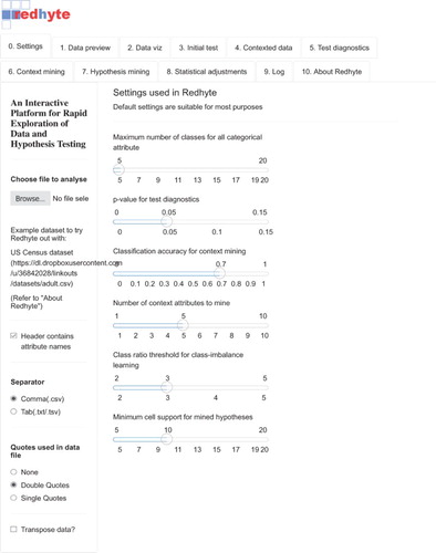
Redhyte has been developed as a web application. That is, it renders in a web browser, such as Google Chrome or Mozilla Firefox. Redhyte’s user-facing interface is organized into tabs, each of which houses a specific functionality that Redhyte provides. As shown in Figure 1, the tabs are arranged, from left to right, according to the following expected workflow of an analysis: A user typically first makes some brief checking and exploration of his input data; this step corresponds to the data-preview and data-visualization modules. The user then specifies his initial hypothesis; this step corresponds to the initial-tests module. Once the initial hypothesis is known, Redhyte analyses it, assesses its validity, generates corrections where necessarily, and mines for interesting related hypotheses. These processes are performed by Redhyte in the background, and require no intervention by the user. After these processes are completed, the user looks at the validity assessments of the test on his hypothesis; this step corresponds to the test-diagnostic module. And he gets information on factors that could strengthen or contradict his hypothesis; this step corresponds to the context-mining module. Finally, the user also looks at related hypothesis mined for deeper insight into his initial hypothesis; this step corresponds to the mined-hypothesis formulation and scoring module.

Figure 1. A screenshot of Redhyte.

Initial hypothesis set-up and tests

The interactions begin with the user loading the input dataset that he wants to analyze into Redhyte. After the input dataset is loaded, the user can proceed to setting up his initial hypothesis. The user uses the Redhyte graphics interface to specify his hypothesis.

In Redhyte, a hypothesis has three components, which are ‘context attribute’, ‘comparing attribute’, and ‘target attribute’. We define these terms by way of the following example: A hypothesis comparing the age at death between smokers and non-smokers amongst the males only, would have the age at death as the target attribute, smoking status as the comparing attribute, and gender as the context attribute.

We use the notations from Liu, Zhang, Feng, Wong, and Ng (2015). Specifically, we use the notation H = ⟨P, A_diff = v₁|v₂, A_target = v_target⟩ to denote a hypothesis H, where P is the context, A_diff is the comparing attribute, A_target is the target attribute, and v₁, v₂, and v_target are attribute values. The context P is itself written as a set of context items of the form attribute = value, for example, {gender = male}.

The meaning of a hypothesis H = ⟨P, A_diff = v₁|v₂, A_target = v_target⟩ is as follows. Each item attribute = value in the context P is interpreted as a condition for selecting a subset of subjects from the input dataset, and the context P is interpreted as the conjunction of all the context items contained therein. Thus the context P represents the subset of the subjects in the input dataset that satisfies all the conditions in P. The comparison A_diff, = v₁|v₂ specifies two subpopulations of P to be compared. The first subpopulation is the subset of the subjects in the input dataset that satisfies all the conditions in P and also the condition A_diff = v₁; we denote this subpopulation as P₁ = P ∪ {A_diff = v₁}. The second subpopulation is the subset of the subjects in the input dataset that satisfies all the conditions in P and also the condition A_diff = v₂; we denote this subpopulation as P₂ = P ∪ {A_diff = v₂}. The target A_target = v_target specifies the condition that we want to compare these two subpopulations on. So H corresponds in the statistical parlance to the null hypothesis that the two subpopulations P₁ and P₂ satisfy the condition A_target = v_target equally well, with the corresponding alternate hypothesis that the two subpopulations P₁ and P₂ do not satisfy the condition A_target = v_target equally well (i.e. the subpopulation P₁ differs from the subpopulation P₂ with regard to the condition A_target = v_target).

Test diagnostics

After the hypothesis is set up, an initial t-test or χ² test is used to test the hypothesis, depending on whether the target attribute is numerical or categorical. The test-diagnostics tab is for making an assessment on whether this initial choice of statistical test meets the requirement/assumptions of the test and, if necessary, also replaces it with a more appropriate statistical test. This assessment is based on the following rules:

• If the initial test is a t-test (Gosset, 1908), the assumptions of normal distributions and equal variances are checked, by using the Shapiro–Wilk test (Shapiro & Wilk, 1965) and F-test (Fisher, 1924) respectively. If either test is significant, the initial statistical test is replaced using the Wilcoxon rank-sum test (Mann & Whitney, 1947), the non-parametric equivalent of the t-test.

• If the initial test is a ‘collapsed’ χ² test (Pearson, 1900), Redhyte computes the individual χ² contributions of each class in the comparing attribute. A collapsed χ² test refers to a χ² test where one or both groups in the initial hypothesis consist of more than one class of the comparing attribute.

• In both cases, the Cochran–Mantel–Haenszel test (Cochran, 1954) is further used on other attributes in the dataset, to assess whether the effect of the comparing attributes on the target attribute is influenced by these co-variates.

Context mining

Redhyte uses classification models for identifying potential confounding attributes to the initial hypothesis. Specifically, it constructs two random-forest (Breiman, 2001) models to model the target and comparing attribute, using all attributes not used in the initial hypothesis. The idea is as follows: if an attribute A is useful both for classifying the target and the comparing attribute, then A might possibly be related to either of them. Therefore it will be interesting to consider using A as an additional context attribute for the initial hypothesis. Random-forest models give variable-importance measures that can be used to rank the attributes by how well they contribute to the classification of the target and comparing attributes. Shortlisting the top few attributes based on the variable-importance measure gives the mined context attributes.

Mined-hypothesis formulation and scoring

The mined context attributes are then individually used as additional context attributes and inserted into the initial hypothesis to form mined hypotheses, by means of stratification. For example, if gender is a mined context attribute, then examples of mined hypotheses could be restricting the initial hypothesis to all males only or all females only. Stratification due to a mined hypothesis can result in one of the following three outcomes: The trend observed in the original hypothesis could be either (i) amplified, (ii) unchanged, or (iii) reversed (Simpson’s reversals). The mined hypotheses – there can be many of these – are ranked using various hypothesis-mining scores (viz. difference lift, contribution, independence lift, and adjusted independence lift) to evaluate which of these three outcomes they fit.

The ‘difference lift’ and ‘contribution’ scores are given by Liu et al. (2015). Difference lift compares a hypothesis H = ⟨P, A_diff = v₁|v₂, A_target = v_target⟩ with a new hypothesis H∗ = ⟨P∪{A = v}, A_diff = v₁|v₂, A_target = v_target⟩, which has an extra item A = v in its context, to see whether the trend specified in H has changed (amplification or reversal) substantially in H∗. To illustrate, consider the contingency tables in Figure 2:

Figure 2. Example contingency tables.

The difference lift is given by , where and are the respective proportions for A_target = v_target in the first contingency table, and and are the respective proportions for A_target = v_target in the second contingency table. On the other hand, contribution measures the change in trend in a way that is weighted by the subpopulations being compared in H and H^∗, and is given by , where n_i and are respective row sums of the contingency tables.

We find that there are situations where contribution disagrees completely with difference lift (e.g. the former reports a negative change in trend whereas the latter reports a positive change). So we also use the ‘independence lift’ and ‘adjusted independence lift’ scores. The derivations and definitions of these are provided in full in the appendix as well as in the full Redhyte report (Toh, 2015). Briefly, the independence lift is given by the difference lift multiplied by the factor , while the adjusted independence lift is given by the difference lift multiplied by. The additional terms multiplied to the difference lift allow both the independence lift and adjusted independence lift to always agree with difference lift in the direction of the change in trend while also take into consideration the sizes of the subpopulations being compared in H and H^∗.

Each of these scores or metrics is essentially used to capture and rank the mined hypotheses in different aspects of ‘interestingness’: viz. trend changes, relative support, and ‘shrinkage manner’. Figure 3 summarizes these metrics and the aspects of interestingness that each metric captures. These interestingness aspects are further elaborated below.

Figure 3. Summary of the various hypothesis mining used in Redhyte.

Trend changes

Trend changes refer to changes in proportions or trends, be it amplifications or reversals, when a mined context item is added into the initial hypothesis. Trend changes are captured by the difference lift, the independence lift, and the adjusted independence lift. Specifically, each of these scores is proportional to change in trend, and has a property that if a Simpson’s reversal occurs, these scores are numerically negative. This property gives us a simple and quick way to detect Simpson’s Reversals.

Relative support

If the mined hypothesis, after the addition of a mined context item, still retains a large support relative to that of the initial hypothesis, then intuitively the mined hypothesis could be more interesting to consider, as it still retains some form of generality. In contrast, if the subpopulations of the mined-hypothesis shrink to a very small number of samples, then this mined hypothesis could be too specific, less useful, and hence less interesting.

The contribution and independence lift of a context item are proportional to the relative support of the mined hypothesis formed by it. In particular, both metrics favours H* with larger relative support, using, for instance, the coefficient in independence lift where is the support for the mined hypothesis while is that of the initial.

Shrinkage manner

When a mined context item is added into the initial hypothesis, the subpopulations of the resultant hypothesis shrink. Consider the following: the context item could, for example, shrink each cell count of the contingency table of the initial hypothesis, in a more or less uniform manner; perhaps subtracting very similar numbers of samples from each cell count. We call this ‘undirected shrinkage’. On the other hand, the context item might also shrink each cell count of the initial hypothesis in a more ‘directed’ manner, whereby a particular cell in the contingency table shrinks much more than the other cells. We call this ‘directed shrinkage’.

The adjusted independence lift is designed to capture directed shrinkage. Specifically, the adjusted independence lift of a context item is proportional to the extent of directed shrinkage that it induces. Intuitively, directed shrinkage could be more interesting as it suggests a strong association of the mined context attribute or item with the initial hypothesis. However, this depends on the domain and the context. As an example, consider the contingency table in Figure 4.

Figure 4. Example of undirected shrinkage.

In this example, the context item I shrinks each cell of the initial hypothesis by five samples, a case of undirected shrinkage. Given such a hypothesis, the adjusted independence lift interprets I and the target attribute T as not associated, and hence it is weighted down in interestingness, with the adjusted independence lift being 0.05. On the other hand, , and the difference lift being 1.31, that is, the trend observed has been amplified by I. In this case, the difference lift and the adjusted independence lift give conflicting conclusions, and without any domain knowledge input, it is arguable that both directed and undirected shrinkage can be interesting.

Statistical adjustments

Other than inserting the mined context items into the initial hypothesis to look into issues such as Simpson’s reversals, we can also control for these mined context attributes by adjusting them using some regression model. The regression model is constructed using the target attribute as the response variable and the mined context attributes as predictors. We call this resultant model the adjustment model. Depending on the type of the target attribute (numerical or categorical), either a linear regression (Freedman, 2009) or a logistic regression (Cox, 1958) model is used.

To construct the adjustment model, Redhyte first uses the stepwise regression algorithm to further shortlist a subset of the mined context attributes to be used in the adjustment model. The construction of the adjustment model and its use are as follows:

• For numerical target attributes, a linear regression model is built such that the target attribute is used as the dependent variable and the shortlisted mined context attributes, with all pairwise interaction terms, are used as covariates. The constructed adjustment model then gives the required numerical adjustments of the target attribute (computed as actual values found in dataset minus fitted values from model). A t-test is then done on the numerical adjustments, to compare with the initial t-test.

• For categorical target attributes, a logistic regression model is built such that the target attribute is used as the dependent variable, while the shortlisted mined context attributes and the comparing attribute, with all pairwise interaction terms, are used as covariates. The constructed adjustment model then gives us a way to treat the entire dataset as if it consists of samples that differ only in the target and the comparing attribute. Such a dataset would be ideal for testing the initial hypothesis. For instance, if the mined context attributes are gender and smoking status, we can analyse the entire dataset as if consists of samples that are all males and all smokers: the logistic regression model gives us a way to conduct such an analysis, by ‘substituting’ these covariate values into the model equation.

Use-case

In this section, we go over a use-case for hypothesis mining with Redhyte. The use-case is based on the adult dataset from the UCI machine learning repository, which can be downloaded at http://archive.ics.uci.edu/ml. This dataset contains the demographical data of 32,561 adults. The target attribute in this dataset is the binary attribute INCOME, which takes as possible values ‘> 50K’ and ‘≤ 50K’. Consider the hypothesis below as our running example:

In the context of {RACE = White}, is there a difference in INCOME between >50 K and ≤50 K when comparing the samples on OCCUPATION between Adm-clerical and Craft-repair?

Initial test

The initial test indicates that the relationship between INCOME and OCCUPATION is significant (p < .05), with white administrative clerks earning less than white craft repairers; see Figure 5.

Figure 5. Contingency table of the initial hypothesis.

Using default settings, Redhyte identifies five mined context attributes after context mining; these mined context attributes are SEX, RELATIONSHIP, WORKCLASS, EDUCATION, and EDUCATION.NUM. In particular, the context items SEX = Male, SEX = Female and WORKCLASS = Self-emp-not-inc give rise to the three contingency tables shown in Figure 6.

Figure. 6. Contingency tables of mined hypothesis with SEX = Female, SEX = Male, and WORKCLASS = Self-emp-not-inc.

These three tables illustrate two instances of a Simpson’s reversal (Simpson, 1951). The first two tables reveal that with respect to neither males nor females do white administrative clerks earn less than white craft repairers, thus invalidating the initial conclusion that ‘white administrative clerks earn less than white craft repairers’. In the third table, the unincorporated self-employed work class results in a completely opposite trend of white administrative clerks earning more than white craft repairers; this is interesting because it highlights the unincorporated self-employed work class as an exception to the initial conclusion that ‘white administrative clerks earn less than white craft repairers’.

Hypothesis-mining metrics

The hypothesis-mining metrics are evaluated on the three items SEX = Male, SEX = Female, and WORKCLASS = Self-emp-not-inc; see Figure 7. These mined hypotheses along with 27 other mined hypotheses are scored using the hypothesis-mining metrics discussed earlier as well as their associated p-values. Redhyte permits the user sorting these mined hypotheses by any of these scores, making the mined hypotheses easier to inspect.

Figure 7. Hypothesis-mining metrics evaluated for the selected context items.

For example, sorting by independence lift brings WORKCLASS = Self-emp-not-inc to the top. This draws attention directly to its large negative value of independence lift, indicating the unincorporated self-employed work class is strongly contradicting (i.e. exhibits a strong trend opposite to) the initial hypothesis that ‘white administrative clerks earn less than white craft repairers’.

On the other hand, sorting by contribution brings SEX = Male and SEX = Female to the top, and the large magnitude of their contribution values suggests each of these subpopulations constitutes a large proportion of the original population in the context of the initial hypothesis. Moreover, the large negative contribution of SEX = Male implies that this subpopulation is dominated by those corresponding to the second row of its contingency table (viz. Craft repair); that is, a large proportion of white males is craft repairers. In contrast, the large positive contribution of SEX = Female implies that this subpopulation is dominated by those corresponding to the first row of its contingency table (viz. Adm-clerical); that is, a large proportion of white females is administrative clerks. Such an imbalance suggests the initial hypothesis that ‘white administrative clerks earn less than white craft repairers’ might be confounded by sex.

Statistical adjustments

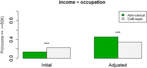
Next we look at statistical adjustments produced by Redhyte. The mined context attributes SEX, RELATIONSHIP, WORKCLASS, and EDUCATION are adjusted in analysing the initial hypothesis. Since the target attribute, INCOME, is categorical, the adjustment model is a logistic regression model. In particular, as shown in Figure 8, after adjusting for SEX = Male, RELATIONSHIP = Husband, WORKCLASS = Self-emp-not-inc, and EDUCATION = Bachelors, a Simpson’s reversal is observed in the initial hypothesis, and points to the opposite conclusion that administrative clerks earn more than craft repairers.

Figure 8. A visualization show the proportions of administrative clerks and craft repairers earning more than 50k, before (left chart) and after (right chart) adjusting for SEX, RELATIONSHIP, WORKCLASS, and EDUCATION.

Conclusion

Hypothesis testing is one of the key tools in data analysis, allowing the analyst to compare different groups of samples. The main steps of a typical data-analysis workflow are: (i) having a scientific question in mind, (ii) formulating an assertion or hypothesis, (iii) collecting and cleaning relevant data, and finally (iv) testing the hypothesis using statistical techniques to decide whether to reject the hypothesis. Most importantly, collection of data in conventional data-analysis settings are often driven by domain requirements and scientific questions a priori.

From a statistical viewpoint, having some initial scientific questions to drive the collection of data means that the collected data are well specified. More precisely, issues such as lack of independence, dissimilar distributions, unequal variances, and class imbalance can be addressed and alleviated using proper sampling methods. However, the big-data setting brings about some interesting and challenging scenarios, such as the collection of data without a scientific question a priori and the ‘large p, small n’ phenomenon (West, 2003).

Collecting data in the absence of an initial scientific question leads to a problem: Assumptions of many statistical techniques, including hypothesis testing, are more often violated than not. Furthermore, having a large number of attributes in a dataset requires appropriate treatment and analysis, in order to account for them. Using a small number of attributes to formulate a hypothesis from a large dataset is not only wasteful, but flawed (due to issues such as confounding factors becoming hidden). For instance, given a hypothesis concerning two attributes, say A and B, for a certain class of a third categorical attribute C, the initial hypothesis could be amplified, that is, the trend observed between A and B is strengthened or reversed, when we consider the class C. In particular, a reversal of trends is known as a Simpson’s Reversal (Pavlides & Perlman, 2009). As illustrated in the use-case earlier, while initial observations suggest that craft repairers earn more than administrative clerks (cf. Figure 5), the complete opposite emerges after automated detection and adjustments are done by Redhyte (cf. Figure 8). There is no known systemic manner of revealing such phenomena, leaving discoveries of such phenomena to pure intuition or chance. A classic example of such a phenomenon is the UC Berkeley gender-bias case (Bickel, Hammel, & O’connell, 1975).

In this paper, we have introduced Redhyte, a platform for statistical hypothesis testing on datasets collected without initial scientific questions. The workflow in Redhyte is as follows: (i) User first suggests an initial hypothesis, which is likely to be rough, intuitive, or domain knowledge-driven. (ii) Redhyte first works on an initial statistical test on the initial hypothesis, and assesses the validity of the statistical test applied to the initial hypothesis. (iii) Redhyte uses data-mining techniques to search for potential confounding attributes (context mining), and uses them to form variants of the initial hypothesis, using stratification. These variants of the initial hypothesis are then scored and ranked, to let the user hone into the more interesting ones. (iv) Finally, Redhyte adjusts for these potential confounding attributes using statistical regression.

Data analysis can be an error-prone process. Unfortunately, while powerful statistical software – e.g. R, Minitab and SPSS – remove a lot of the difficulties in the process, they do not check whether the user is applying the statistical tests correctly. A key differentiation of Redhyte is that Redhyte supports the checking of whether the user is working on the analysis correctly, guides him to do his statistical test correctly, and recommends related hypotheses that are potentially deeper and more insightful. Redhyte is therefore one step towards building a self-diagnosing, self-correcting, and helpful analytic system, though it currently supports only simple statistical tests.

On the data-mining side, the closest work related to Redhyte is perhaps the work of Liu et al. on exploratory hypothesis testing and analysis (Liu et al., 2012, 2015). In these works, Liu et al. describe algorithms for the mining and visualization of hypotheses from large datasets. Furthermore, they also presented algorithms for linking together related hypotheses and measures for ranking hypotheses (we have proposed refinements of these here and implemented them in Redhyte). Works from clustering, grouping of frequent itemsets, and association rules (Liu, Zhang, & Wong, 2014; Poernomo & Gopalkrishnan, 2009; Wang & Parthasarathy, 2006; Yan, Cheng, Han, & Xin, 2005) are also useful for generating related hypotheses. However, we do not consider these clustering methods here because we start from a single user-specified hypothesis. Therefore, we face a much lower mining and clustering complexity. Last but not least, these methods are not concerned with ensuring the validity of a user’s statistical test or guiding him towards a valid statistical test.

Disclosure statement

No potential conflict of interest was reported by the author(s).

Notes on contributors

Wei Zhong Toh is an Analytics Product Manager at NCS Group, managing various data- and analytics-driven products in the data science team. He was previously a data science consultant, and has worked on industrial projects spanning Smart City analytics, Geospatial analytics, and Telecommunication analytics. The idea of Redhyte was co-conceived as part of his exploration of exploratory hypothesis testing and analysis. Wei Zhong holds a Bachelor of Science (First Class Honours) in Computational Biology from the National University of Singapore and is currently pursuing a Master of Science in Statistics from NUS.

Kwok Pui Choi is an Associate Professor of the Departments of Statistics and Applied Probability and of Mathematics, National University of Singapore. His research interests include probability, statistics, computational biology and statistical bioinformatics.

Limsoon Wong is Kwan-Im-Thong-Hood-Cho-Temple Chair Professor at the Department of Computer Science, National University of Singapore. He currently works mostly on knowledge discovery technologies and their application to biomedicine. He is a Fellow of the ACM, inducted for his contributions to database theory and computational biology.

Additional information

Funding

LW gratefully acknowledges funding support from the Kwan Im Thong Hood Choo Temple, Singapore chair professorship and Ministry of Education - Singapore tier-2 grant MOE2012-T2-1-061. WZT gratefully acknowledges funding support from NCS Pte Ltd, Singapore.

Appendix

Difference lift and contribution

Given the initial hypothesis in a 2 × 2 contingency table,

Table

	Target attribute class	Target attribute class
Comparing attribute class
Comparing attribute class

where(A1) Adding a context item },

Table

	Target attribute class	Target attribute class
Comparing attribute class
Comparing attribute class

where and and as similarly defined:(A2) The first hypothesis-mining metric, defined in Liu et al., is the difference lift, as follows:(A3) The difference lift takes into account the change in trend in the mined hypothesis , when a context item is added into the initial hypothesis. In particular, if(A4) then a Simpson’s Reversal occurs. Intuitively, for a mined hypothesis , we would like to evaluate its interestingness at least by three different measures: (i) whether the trend has been reversed, (ii) whether the change in trend (trend amplification or reversal) is substantial, and (iii) whether the subpopulations of are still large enough. The difference lift is able to account for the first two measures, but not the third.

Liu et al. defined the second hypothesis-mining metric, contribution, as follows:(A5) Contribution, while considering the subpopulation sizes in , loses the property that difference lift has in (A4). For example, given ,

We get

The latter may be negative, depending on and .

Derivation of independence lift

Consider : (A6) Likewise,(A7) By Bayes Theorem,(A8) (A9) By the definition of independence, and are independent ifTherefore, is a measure of association/independence between and . We would like to call as the independence factor of on . can be easily computed from the contingency table of :(A10) Likewise, the independence factor of on , and is a measure of association/independence between and:(A11) The difference can be considered to be a form of measure of the differential extent of association/independence that has on and . In the same manner, and are defined accordingly.

We next define the independence lift to be(A12) The term allows for to be evaluated on relative subpopulation sizes in comparison to . In addition, by (A8),(A13) where(A14) (A12) and (A13) imply that the independence lift acquires the property of the difference lift shown in (A4), while being able to account for changes in subpopulation sizes.

Derivation of adjusted independence lift

Consider the following: is the independence factor of the context item on . If , and are independent. This implies that the removal of subjects from the subpopulations of , by adding the context item , to form is more ‘haphazard’, as compared to if . We call the case when or when is close to 1, undirected shrinkage of subpopulations. When is far from 1, we call that directed shrinkage. Under undirected shrinkage, the removal of subjects from was not influenced by the context item , and hence we might say that if was (in)significant in the first place, then is likely to be (in)significant as well. Therefore, a mined hypothesis would be more interesting if, or equivalently,, deviates as far away from as possible, that is, direct shrinkage. Based on this intuition, we define the adjusted independence lift:(A15) In all, Redhyte uses the above four hypothesis-mining metrics, which are the difference lift, contribution, independence lift, and adjusted independence lift, in addition to the χ² test statistic and the (adjusted) p-values, to evaluate the interestingness of mined hypotheses.

References

- Bickel, P., Hammel, E., & O’connell, J. (1975). Sex bias in graduate admissions: Data from Berkeley. Science, 187, 398–404. doi: 10.1126/science.187.4175.398
- Breiman, L. (2001). Random forests. Machine Learning, 45, 5–32. doi: 10.1023/A:1010933404324
- Cochran, W. G. (1954). Some methods for strengthening the common χ2 tests. Biometrics, 10, 417–451. doi: 10.2307/3001616
- Cox, D. R. (1958). The regression analysis of binary sequences (with discussion). Journal of the Royal Statistical Society B, 20, 215–242.
- Fisher, R. A. (1924). On a distribution yielding the error functions of several well-known statistics. Proceedings of the International Congress of Mathematics, 2, 805–813.
- Freedman, D. A. (2009). Statistical models: Theory and practice. Cambridge University Press.
- Gosset, W. S. (1908). The probable error of a mean. Biometrika, 6, 1–25. doi: 10.1093/biomet/6.1.1
- Ioannidis, J. P. A. (2005). Why most published research findings are false. PLoS Medicine, 2, e124. doi: 10.1371/journal.pmed.0020124
- Liu, G., Suchitra, A., Zhang, H., Feng, M., Ng, S. K., & Wong, L. (2012). AssocExplorer: An association rule visualization system for exploratory data analysis. Paper presented at the proceedings of 18th ACM SIGKDD conference on knowledge discovery and data mining, Beijing, China, pp. 1536–1539.
- Liu, G., Zhang, H., Feng, M., Wong, L., & Ng, S. K. (2015). Supporting exploratory hypothesis testing and analysis. ACM Transactions on Knowledge Discovery from Data, 9, article 31. doi: 10.1145/2701430
- Liu, G., Zhang, H., & Wong, L. (2014). A flexible approach to finding representative pattern sets. IEEE Transactions on Knowledge and Data Engineering, 26, 1562–1574. doi: 10.1109/TKDE.2013.27
- Mann, H. B., & Whitney, D. R. (1947). On a test of whether one of two random variables is stochastically larger than the other. Annals of Mathematical Statistics, 18, 50–60. doi: 10.1214/aoms/1177730491
- Pavlides, M., & Perlman, M. (2009). How likely is Simpson’s paradox? The American Statistician, 63, 226–233. doi: 10.1198/tast.2009.09007
- Pearson, K. (1900). On the criterion that a given system of deviations from the probable in the case of a correlated system of variables is such that it can be reasonably supposed to have arisen from random sampling. Philosophical Magazine Series 5, 50, 157–175. doi: 10.1080/14786440009463897
- Poernomo, A. K., & Gopalkrishnan, V. (2009). CP-summary: A concise representation for browsing frequent itemsets. Paper presented at the proceedings of 15th ACM SIGKDD international conference on knowledge discovery and data mining, Paris, France, pp. 687–696.
- Shapiro, S. S., & Wilk, M. B. (1965). An analysis of variance test for normality (complete samples). Biometrika, 52, 591–611. doi: 10.1093/biomet/52.3-4.591
- Simpson, E. H. (1951). The interpretation of interaction in contingency tables. Journal of the Royal Statistical Society B, 13, 238–241.
- Toh, W. Z. (2015). Redhyte: an interactive platform for rapid exploration of data and hypothesis testing. Project report, National University of Singapore. Retrieved from http://www.comp.nus.edu.sg/~wongls/psZ/tohweizhong-fyp2015.pdf
- Toh, W. Z., Choi, K. P., & Wong, L. (2016). Redhyte: Towards a self-diagnosing, self-correcting, and helpful analytic platform. Paper presented at the proceedings of 8th Asian conference on Intelligent Information and Database Systems (ACIIDS 2016), Part II, pp. 3–12, Da Nang, Vietnam.
- Wang, C., & Parthasarathy, S. (2006). Summarizing itemset patterns using probabilistic models. Paper presented at the proceedings of 12th ACM SIGKDD international conference on knowledge discovery and data mining, Philadelphia, PA, pp. 730–735.
- West, M. (2003). Bayesian factor regression models in the “large p, small n” paradigm. Bayesian Statistics, 7, 723–732.
- Yan, X., Cheng, H., Han, J., & Xin, D. (2005). Summarizing itemset patterns: A profile-based approach. Paper presented at the proceedings of 11th ACM SIGKDD international conference on knowledge discovery and data mining, Chicago, IL, pp. 314–323.