Audio fingerprint hierarchy searching strategies on GPGPU massively parallel computer

ABSTRACT

Audio fingerprint was developed for representing the audio based on the content of waveform. With the audio fingerprint database, we can easily manage the song/music with high reliability and flexibility. However, with the well-developed Internet of today, the audio data have become bigger and bigger which make the management of audio/music data more difficult. There are two problems that we need to solve when the audio fingerprint database turn into bigdata: the size of the database needs to be sufficient for storing 10 millions of audio fingerprint and the strategies for searching the nearest song in acceptable time for thousands of queries at once [Nguyen Mau, T., & Inoguchi, Y. (2016). Audio fingerprint hierarchy searching on massively parallel with multi-gpgpus using K-modes and lsh. Eighth international conference on knowledge and systems engineering (KSE) (pp. 49–54). IEEE]. In this research, we propose the methods for storing the audio fingerprint using multiple GPGPU and nearest song searching strategies based on these databases. We also showed that our methods have the significant result for deploying the real system in the future.

KEYWORDS:

• Audio fingerprint
• massively parallel
• parallel processing
• GPGPU
• compute unified device architecture (CUDA)
• K-modes
• K-means
• locality sensitive hashing (LSH)

1. Introduction

The main target of the algorithm for audio fingerprint extraction is the ability to standardize the content of music/audio. A good audio fingerprint algorithm extraction can represent the music/audio from a complex domain of waveform into a new feature-based domain that can support comparing the similarity and difference of two songs/audio from every particular part of its audio fingerprint. In this paper, we use HiFP2.0 as the audio fingerprint extraction algorithm for the detection of the distorted audio from the original audio file. We inherited the advantages of the HiFP2.0 algorithm for extracting the audio fingerprint and focussing on proposing a new intelligent storage of fingerprints for the computer using multiple GPGPUs and having to accommodate the parallel nearest problem algorithm that can support to handle numerous queries at the same time (Yang, Sato, Tan, & Inoguchi, 2012).

In Figure 1 is shown the audio fingerprint searching system consisting of two main stages: firstly, we use one audio fingerprint extraction for generating the audio fingerprint for the unknown audio. The second stage is using the searching strategy for searching the query audio fingerprint with the big database with the labelled audio fingerprints of the original song/audio. With the returning of the information of the nearest audio fingerprints on the database, we can conclude on the metainformation of the query unknown audio.

Figure 1. Audio fingerprint searching problem.

Considering the targets of the audio fingerprint searching system, first of all, the accuracy of the system should be emphasized. Because in the real case, the audio/song can be transformed by different ways such as changing of pith/volume, adding noise, or blening with other audios/songs (Cano, Batle, Kalker, & Haitsma, 2002). In that case, we should choose the audio fingerprint extraction algorithm with high reliability accuracy and combine with the outstanding searching algorithm to make sure to have the right nearest song/audio. Secondly, with the complexity of the extraction and searching stage, we need to increase the performance by decreasing the extraction and searching time for using a large amount of audio fingerprints on the database and numerous queries at the same time. To do that we encouraged the use of the computer with multiple GPGPU devices for dividing the database into multiple sub-databases and parallelly the searching stage into multiple threads for queries with hierarchy architecture by using the cores of GPGPU devices.

In our research, we increase the speed by parallelism; however, the role of CPU is very important for the management of the flow of queries and the threads of devices also. Based on that we divided our system into two levels: ‘Level 1’ is the management level which is executed by the CPU and each ‘Level 2’ for each GPGPU device that can work independent of each other.

In a previous work, we proposed the data structure for storing the audio fingerprint database on the CPU–GPU system and approach for fast massively searching multiple queries (Mau & Inoguchi, 2016b). In this research, we continue to improve the system by caching memory and transferring between GPUs. In addition, we proposed the optimization methods for getting a better accuracy and performance. There were still two main problems in our previous work that were solved in this research. Firstly, we extended the clustering algorithm for achieving the desired size for every cluster, because the size of the GPU device is limited and the existing variants of the K-mean clustering algorithm do not support this requirement. Secondly, our system is a complexity system that consists of multiple sub-databases, using the broadcast query for every sub-dataset is good for a high-performance system. In this paper, we also proposed strategies for searching with cluster aware by query and the passing method for audio fingerprint query from one GPU device to another GPU device to get the best accuracy.

2. Research background

The audio fingerprint database F includes a great number of points (also known as audio fingerprint) n: . The metainformation for all original audio fingerprints in F is given as well. We implement to search the nearest audio fingerprint in F and use its metainformation for the corresponding query with the goal of showing the metainformation of multiple unknown metainformation queries (audio fingerprints) . There are two requirements in this research: the average searching time needs to be below the threshold (1 s) for big database (10-million fingerprint database) and the need to support process multiple queries at the same time in parallel processing. There are two main problems when doing this searching system: intelligent distributed storage for multiple devices and strategies for parallel searching among two levels with multiple sub-databases.

2.1. Audio fingerprint

Audio fingerprint is a digital vector that was extracted from the audio/song waveform and able to standardize the content of the audio/song source. Audio fingerprint can easily help for comparing the similarities and differences of songs. In addition, using audio fingerprint for storing can reduce the size of original audio/song with the standard structure. In our system's database, instead of storage the real waveforms of the songs we considered storage of the audio fingerprints and its metainformation for every song/track.

In Figure 2, there is an audio fingerprint that is represented by a binary sequence extracted by HiFP2.0 fingerprint extraction algorithms. This audio fingerprint is extracted from first 2.97 s of a song and that can reduce the size of song by 512 times (Yang et al., 2012).

Figure 2. An example of 4096 bits fingerprint extracted by the HiFP2.0 fingerprint extraction algorithm.

Using audio waveform for comparing may have many difficulties because that it is un-normalized, so we favour to use audio fingerprint for storing and processing in our system. The features below are the singularities of audio fingerprint that need attention:

• Robustness: Fingerprint can identify the audio even if the audio has been transformed in many ways or has noise.

• Fingerprint size: The number of songs is plenty but the memory of the device is limited, so it is very important when we build the real system.

• Granularity: Due to the normalized format, the comparison of audio fingerprints can be much simpler than comparing the audio waveform.

• Search speed and scalability: Searching time depends much on the size of the database and the method to search. And audio fingerprint can be extracted form multiple variances of music for conducting a normalized audio fingerprint.

• Efficient comparison: Audio fingerprint extraction algorithm focuses on removing the irrelevant information from the content, so this will be more efficient than comparing the information with distortion data.

2.2. HiFP2.0: an audio fingerprint extraction algorithm

There are several audio fingerprint extraction algorithms such as Mel Frequency Cepstral Coefficients (MFFC) (Seo et al., 2005) and Linear Predictive Coding (Cano et al., 2002). Each audio fingerprint extraction algorithm has its advantages and disadvantages and can be applied in different fields. Most of the audio fingerprint extraction algorithms use the fast Fourier transform (FFT) to transfer to the spectra domain before extracting the features.

Using FFT has problem about the performance, with the complexity of it is not suitable for the system's need instant response. Especially when dealing with big queries such as audio waveform. Besides that FFT uses floating-point operations as principle calculation that can increase the processing time and take more memory storage. In order to decrease processing time by avoiding a highly complex algorithm and floating-point operations, we decided to use Haar Wavelet Transform (HWT) instead of the FFT process. HWT converts PCM to time–frequency domain and dominant by integer operations (Jain, Araki, Sato, & Inoguchi, 2011).

We chose to use HiFP2.0 for the Achieve the audio fingerprint from audio waveform. HiFP2.0 of Araki can process without the floating-point operations being used. A fingerprint size is just 512 bytes, which is small for storage. This is good for a low-memory capacity computer. The results also show a good result with acceptable ratio (Jain et al., 2011; Yang et al., 2012).

Algorithm 1 MHWT: Algorithm of multi-level sub-band decomposition using Haar Wavelet Transform)

Require: wav[]← input waveform data, n← number of input signal, m ← number of output samples  while TRUE do   n ← n/2;   for i = 0; i <n/2; i++ do    Hi[i]← ( wav[2*i] − wav[2*i+1] ) / 2;    Lo[i] ← ( wav[2*i] + wav[2*i+1] ) / 2;   end for   wav[]← Lo[i];   if n < m then    break;   end if end while return (Hi, Lo);

Algorithm 2 Algorithm of HiFP2.0 audio fingerprint generation)

Require: wav[]← PCM data  n ← Number of PCM data samples;  m ← Number of output samples;  Hi[], Lo[] ← MHWT( wav[], n, m );  for do   if Lo[i] - Lo[i+4] >0 then    FP[j]← 1;   else    FP[j]← 0;   end if  end for  FPID[m-1]← 0;  return FP;

Algorithm 1 shows the principle procedure of HiFP2.0. First of all, HiFP2.0 uses the HWT to decompose the waveform signal to low frequency and high frequency which have half-length of the input data. It could be used in multiple levels of HWT and with the higher level of sub-band, it needs the result of the previous sub-band level. The number of HWT levels will present the compact size of audio fingerprint after extraction. In our case, we choose the fixed number of the HWT level to be 3 for getting optimal speed and audio fingerprint size.

Algorithm 2 demonstrates how HiFP2.0 uses HWT information for generating the audio fingerprint with binary value: after obtaining the decomposition sub-bands of input waveform, HiFP2.0 eliminates the high-Ffequency sub-band that denotes the noise of input waveform. The next steps are calculating the differences of the continuous low-frequency sub-band with step of four. If the next value of is greater than , then the value of will be assigned by TRUE (ascent). In other way, the corresponding value of will be assigned by FALSE (descent). Similar to MFFC, HiFP2.0 calculates the energy of mutual sub-bands. HiFP2.0’s features only store the gradient values as the binary value (Yang et al., 2012).

After full stage of HiFP2.0 extraction, we will achieve a binary vector that represents the content of the corresponding waveform. In general, for comparing the source audio's size which uses three-level decomposition, HiFP2.0's binary sequence has a size less than 512 times than the original (Yang et al., 2012).

2.3. Locality sensitive hashing

In this research to determine the metainformation of an unknown audio file, we need to find the most similar song for the query by using audio fingerprint. We will consider Nearest Neighbour Search (NNS) for getting the nearest audio fingerprint and ϵ-Nearest Neighbour Search (ϵ-NNS) for getting the ϵ nearest audio fingerprints for the query.

Theorem 2.1 (ϵ-Nearest Neighbour Search(ϵ-NNS)):

Given a set P of objects that are represented as points in a normed space pre-process P in order to return efficiently a point for any given query point q in such a way that , where is the distance from q to its closest point in P (Andoni & Indyk, 2006; Chang, 2011).

In Figure 3, we can see that there are three points in the database and a query point . For the nearest neighbour problem, should be the chosen one. However, when we consider the approximate nearest neighbour problem on this database, suppose that the distance between and is R and the approximate factor is c, there are two points that will meet the requirement . In this case, we can also return or both of which are fine.

Figure 3. An illustration of the nearest neighbour and approximate nearest neighbour (Andoni & Indyk, 2006, p. 2).

LSH is a well-known algorithm to handle the ϵ-NNS problem which uses the approximate nearest neighbour. LSH simply divides the data into multiple buckets, the number of the hash function in the hash family function will indicate the number of buckets in the system. Vectors/points in the same buckets will be similar to each other because of the continuity of the selection of hash functions. Therefore, instead of computing the similarity the input vector with all of the vectors in database, we just need to compare the query with the vectors in several buckets.

With LSH, hash functions will be used for choosing l subnets of database vectors. Let be the projection of vector on the coordinate positions. Then denoting , we store every in the bucket . Since the number of buckets is probably large or the numbers of points in every bucket differ considerably, so another table is also needed to save the map of buckets.

Similar to the searching problem within LSH, the same hash functions are also used for each query. As for the query , we define all , and then let be the points in the bucket on the current process. We have to calculate the distance for each point in this bucket. As for the KNN problem, we do not stop until we reach K points in the same or different buckets. But, with the audio fingerprint, it can be returned at the first having the so as to attain a good result, along with a better performance. Note that in the case the two points are close to each other, is a threshold of the maximum distance.

In Figure 4, LSH chooses a family of the hash function for handling database and query also. In the preprocessing stage, the hash function is used for dividing the database into buckets, there are three buckets with the different colours in the figure. Each bucket will have its hash value by the principle of hash function. In terms of the Searching stage, the query also needs calculating the hash value by the previous hash function. This value of the hash function will indicate a bucket that holds the similar points to the query (bright box). Next, there is another step for comparing the distance from query to all points in the purple buckets and returning the closest one.

Figure 4. An illustration of locality-sensitive hashing.

2.4. K-means

Clustering is used with a view to partition the database points into the distinguished groups. Clustering plays an important role in machine learning, image processing, pattern recognition and data mining. And K-means is one of the most common algorithms to implement data clustering (Tzortzis & Likas, 2008).

Assume that we now have a dataset of fingerprints . This dataset needs dividing into K groups (also called as clusters) . K-means will find the local optimal solutions having minimized error functions that are determined by the sum of Euclidean distances between every data point and , where is the cluster 's mean vector. The error function is determined as follows (Tzortzis & Likas, 2008):(1)

The target of K-means clustering is to find out the model which can minimize the error function (1(1) ):

Choosing the number of cluster K is very important for the cluster optimization, the different datasets have different number K for their most compact optimization. However, in our research, we choose a number of cluster K by the number of GPU in our system that can optimate the performance and system compact. The complexity of K-means is , with i being the number of iterations, if we have a larger number of cluster K it will take more time for building the model and the time for calculating the distance from queries to all centroids. Therefore, we decided to choose using the system which has only one cluster storing on one single GPGPU device.

2.5. K-modes

One of the popular extensions for K-means which concentrates on clustering the discursive data is K-modes. Binary vector being a type of categorical data has two categories: TRUE or FALSE. The labelling step K-means prefers to use distance (known as hamming distance) in order to measure the differences among categorical values:

K-modes employ the same method as K-means in the labelling step. The method being mentioned minimizes the hamming distance for the point to all modes (centroids) . For the updating modes step, the dominant attributes will be found by K-modes in each cluster considering all dimensions so as to set the attribute to centroids vectors. Denoting as a cluster (set) we would like to look for the centroid Q that is the expected centroid for Y. The main aim is to minimize the sum of distance between points and its centroids:

In order to search for the dominant attributes in set F, let be the number of objects in F that has the kth category in attribute and be the frequency of category in F. The gets the minimum value if and only if:

where d is the dimensions of vector.

3. Related works

3.1. Streaming similarity search over one billion tweets using parallel locality-sensitivehashing (PLSH) (Sundaram et al., 2013)

The PLSH system shows that it can handle the database with billions of records by building two levels of LSH. The database is stored in different parts kept in distinguished nodes. PLSH focuses on dealing with the big data such as Tweets' database, the constantly updated data are a problem of LSH due to the transformation of hash table and index of record in the database. Another advantage of PLSH is handling the queries in real time for the requisite of Tweets' users (Sundaram et al., 2013).

According to Figure 5, the coordinator will receive the data from inserting data or search query. For inserting, PLSH uses a filter window to choose M nodes from i to i+M−1 to handle the inserts in a round-robin fashion (Figure 6).

Figure 5. PLSH system (Sundaram et al., 2013, p. 2).

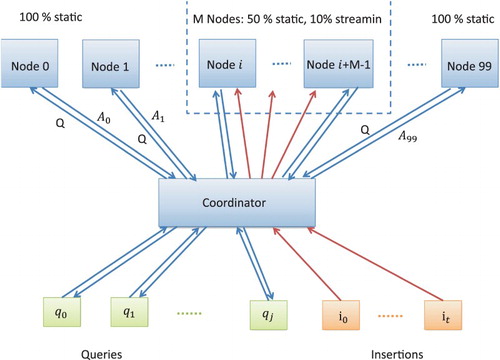
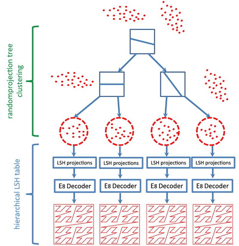
Figure 6. Bi-level LSH using RP-tree and hierarchical lattice (Pan & Manocha, 2012, p. 3).

The authors propose to use two-level hashing to reduce the number of hash construction instead of using many pointers to indicate the address of every bucket. Besides that, partitioning the database can help store the big hash table on several nodes; so the PLSH can work in nodes with small memory. Another strength of PLSH is parallel querying on multiple nodes, each node holds an independent part of the database; so they can search at the same time before sending the result to coordinator. With these advantages, PLSH can speed up the inserting and query stage of Tweet system to 1.5X (Sundaram et al., 2013).

3.2. Bi-level locality sensitive hashing for k-nearest neighbour computation (Pan &Manocha, 2012)

There are two levels of processing in a bi-level LSH algorithm proposed by Pan & Manocha (2012). At the first level, they used random projection tree (RP-tree) for dividing the dataset into subnets. The points on the same subnets tend to be similar to each other because of the strengths of the RP-tree. The authors at the second level built an LSH table for every subnet. Particularly, the authors used a Morton curve for creating a hierarchical LSH in order to raise the speed performance for LSH query. With regard to the k-nearest neighbours' problem, to get k-nearest neighbours when the query has hash value to the bucket under high-density data, the algorithm only needs to search the few nearby buckets. And when the query bucket has low-density data or is empty, the algorithm has to search on farther buckets for getting enough number of nearest neighbours (Pan, Lauterbach, & Manocha, 2010; Pan & Manocha, 2012).

In Figure 6, With the query step, firstly the bi-level LSH algorithm has to compute the RP-tree leaf node containing for the query . Then, LSH at the second level is employed to seek the buckets holding and the hash table that is shown in the RP-tree leaf node at the first level. Hence, the output address for a query embraces two parts described by the following formula: . Here, the is the address of a leaf node that includes , and is the index of the bucket that has in the corresponding subnet. The locality coding of bi-level LSH is better than the one of the original LSH hash function. Moreover, its deviation is also smaller owing to the random projection of the RP-tree. Therefore, it can be said that bi-level LSH is an algorithm which is more suitable for GPU because of the fact that when running on the GPU, it can reach the speed of 40 times faster than running on the CPU (Dasgupta & Freund, 2008; Pan & Manocha, 2011, 2012).

4. Proposed method: HiFP2.0 audio fingerprint database clustering for multipledevices

When coming to the problem of building searching system using multiple GPPGU devices, the first thing we need to do is clustering the database because the memory storage of devices is isolated. In this section, we will show our method for clustering the audio fingerprint into multiple sub-database which supports fast searching and still inherits the goodness of K-means and K-modes. Figure 7 shows that for the binary vectors, generating the initialization centroid in the range of database is quite simple. A subnet of database is represented by a binary vector which minimizes the distance from it to all other points within its cluster. Every sub-database will be transferred to the LSH module to create the buckets hash table after we have K subnets of database (Huang, 2009).

Figure 7. Preprocessing database for hierarchy searching for two devices.

Algorithm 3 Extended K-modes for achieving the desired-size clusters (limited size)

Require: Database,K,M = M1, … ,MK, limited-size of clusters S = S1, … , SK Initialization:  L ← Sorted list of points by the delta of distance from nearest to farthest cluster;  M(, ) ← Sorted list of clusters by distance from nearest to farthest cluster for every points;  For the points p in L: L(p) = M(p, 1) if size(M(p, 1)) < S(M(p, 1));  Loop:  while centroids not change or iteration ≥ iterationmax do    ; For 1 ≤ i ≤ K   L ← Sorted list of points by the delta of distance from nearest to farthest cluster;   for For every points p if L(p) ≠ 0 do    M(p) ←Sorted list of clusters by distance from nearest to farthest cluster for p    if if size(M(p, 1)) < S(M(p, 1)) then     L(p) ← M(p, 1);    end if    if size(M(p, 1)) ≥ S(M(p, 1)) then     if Find M(q) have Distance(q,M(q)) ≤ Distance(q,M(p)) then      Swap(q, p);    end if   end if  end for end while return K Sub-database with limited-size clusters

In Algorithm 3, with K clusters, denotes the labels of cluster i. The new parameters in this algorithm are that is the limited size of cluster i. In the initialization, we need to build the list of points L that are sorted by the delta of distance between closest cluster and farthest cluster. From L, we can build the 2-D list that contains the list of all clusters from the nearest to farthest for all points in L for every point. With the binary dataset, we use the Hamming distance for measuring the distance between two data points. The centroid of a cluster will also be represented as a mean binary vector that helps us to use the hamming distance for computing the distance between a data point and a cluster. After that, we initialize the labels for all data point in L, it will assign p to its nearest cluster if the size cluster is less than its limited size . It is true that some data points will not be assigned to its nearest cluster due to the cluster being full, in that case, it will try to assign the label to the second nearest cluster and so on. In the updating step of this algorithm, we update the centroids with the method of original K-means, the centroid is the mean of all data point . With the changing centroids, we have to re-update the value of list L. The second stage step of K-means is updating the labels for all data points p, in this case, we re-compute the cluster-list . From , we can know if the point p belongs to its nearest cluster or not, if not, we have to check the size of the cluster with its limited size . In case of the cluster being full, we have to find the point q that currently belongs to its nearest cluster with the nearest cluster of q being p's current cluster, then we can safely swap the label of p and q. Similar to K-means, this algorithm will stop when it reaches the maximum number of iterations or the value of centroids is not changed. This algorithm can be used in different datasets with different purposes other than audio fingerprint clustering.

With Algorithm 3, we can separate our original database into multiple sub-databases that can be stored into the limited memory size of a single GPGPU device. And with the advantages of the optimization of points in the same cluster of K-modes, we can use it for building the fast searching system. In Figure 7, With the smaller sub-databases, we can also use our LSH hash functions for building the buckets for each one similar to single GPPGU system.

5. Proposed methods: audio fingerprint hierarchy searching strategies on a GPGPUmassively parallel computer

In this section, we will show our different searching strategies for audio fingerprint on the computer with multiple GPGPUs and show their advantages and disadvantages also.

5.1. Parallel audio fingerprint searching using single GPGPU

The audio fingerprint database stores a limited number of audio fingerprint and metainformation by the memory size of the GPGPU device. The queries of audio fingerprints query have T queries with unknown information. The requirement is to build a audio fingerprint system that returns the information for unknown queries meeting the following conditions:

• Accuracy: The average percentage of right matching with the original song should be acceptable for building the system in real cases.

• Throughput parallel searching: The number of queries at the same time that a system can handle should be large enough to meet the requirements when having multiple access at one.

• Limited database size: The requirement of this section is using only one GPGPU device for searching. For using only one device, we need to notice the memory amount of the current GPGPU device.

• Limited searching time: Searching time is also an important factor that we need to consider. The time for returning the result should be acceptable for real one access time.

5.1.1. Preprocessing the audio fingerprint on single GPPGU

For building the hash table for audio fingerprint data, we need to choose the number of the hash function, this number of family hash function will be also used in the searching stage. The same family hash function is used for every audio fingerprint in data for getting the hash value corresponding to the audio fingerprint. Each different value of hash value will indicate the same bucket address.

We can see in Figure 8, after running the lSH algorithm, we get a hash table that is related to the input data. The database of the searching stage is the combination of the raw data with audio fingerprints and the hash table generated by the raw data by the LSH algorithm. The final step in the preprocessing stage is the loading of the database including the audio fingerprint and hash table into the GPPGU device. With this well-developed database structure, we can easily find the address of buckets and use it to find the addresses of every audio fingerprint in this bucket.

Figure 8. Preprocessing flow for the audio fingerprint searching system using the single GPGPU.

5.1.2. Audio fingerprint searching method on single GPGPU

In Figure 9, in every thread we handle the searching for one query. And the searching stage in one thread returns only one ID for corresponding query. The first step, using the same hash family functions H in the preprocessing step and the same number of hash function, the threads will calculate the hash strings for sub-query from . For each hash string will point to a bucket B that holds several audio fingerprints . For the second step, the thread will compare the distance of query to every audio fingerprint in B to find the distance that meets the threads hold of LSH. This thread will stop when an approximate nearest neighbour is found on any sub-fingerprints's bucket.

Figure 9. Principle of audio fingerprint searching flow in one thread.

5.1.3. CUDA implementation

In every SM for the method, we will be able to divide the job of queries into multiple small jobs for multiple threads. And in this case, with the staged-LSH, it already divides the audio fingerprint into 126 sub-fingerprints. In Figure 10, one query will be handled by 126 threads on the same warp. However, when using the unit thread for sub-fingerprint, it will raise the problem for management of the shared memory for the threads in the same block. Especially, 126 sub-fingerprints for 1 fingerprint, but we only need to return one of the approximate nearest neighbours for the input query. So, we need the shared memory for temporary current approximate nearest neighbour. Then 126-threads are permitted for changing the value of this shared memory. To avoid this, we have to handle the writing process of every thread to this shared memory. This trick will reduce the searching time of the total system.

Figure 10. CUDA threading allocation with using 126 thread – 1 query on multiple SM.

5.1.4. Result of audio fingerprint searching system using single GPGPU

In Figure 11, we tested our method using single GPGPU using a different size of data with the GPGPU details in Table 1. As the number of queries is the same so the size of data copied from the host to the device and data's size of IDs copied from the device to the host are the same for any database. So, the transfer time is similar for every size of the database. We can see that the executed time depended much on the database size and the number of hash functions. For different sizes of data, we should choose a different hash function number for getting the best performance. For example, if we have 1,000,000 audio fingerprints in the database we should choose to use 20 hash functions. But when dealing with database having 10,000,000 audio fingerprints, we should use 24 hash functions for getting the best result (Figure 12).

Figure 11. Transfer and executed time (milliseconds) using single GPGPU (1024 throughput queries).

Figure 12. Accuracy using single GPGPU (1024 queries – 5% Audio Fingerprint Distortion).

Table 1. GPPGUs information are used for testing the K-PLSH.

	GPGPU
Name	Tesla K40
Frequency	745 MHz
Memory	13 GB
Language	Cuda
Cores	2880
Threads	2880
Compiler	nvcc 7.0
OS	CentOS 6.4

The same conditions are used on the test in Figure 11, but in Figure 11 the accuracy depends much on the number of hash functions. With the higher hash function number, the accuracy of the system will be reduced. It can be explained easily by the number of buckets affected by a number of hash functions. With more buckets, the average number of audio fingerprint in a single bucket will be reduced. In this case, the chance for getting the approximate nearest neighbour will also reduce. We can see with 20 hash functions it can achieve high accuracy with acceptable search time. For the next coming result we will use 20 hash functions for another testing. In Table 1, we give the detailed information of GPGPGU devices we used for implementing our experiments.

5.2. Parallel audio fingerprint searching using multiple GPGPUs with K-modesmodel

Similar to K-modes, our proposed clustering algorithm also has the model for structuring the information of cluster and calculating the similarity of point and cluster. We used the distance function of K-modes for computing the distance from the data point to cluster.

The first level for searching the query in the database is K-modes Querying. A controller is needed for handling to query the input value, also distributing it to the suitable second level. The controller has to compute the hamming distance from the query to each centroid for finding closest cluster (Huang, 1998; Huang, 2009).

Because every device has different sub-database and LSH hash table, so LSH query can handle independently every device. With the query , the respective bucket B can be addressed by the same hash value through the functions in the step of preprocessing. As for each point , we have to calculate the hamming distance for indicating which one can meet the threshold in an attempt to return the approximate near neighbour. However, if none of the points is not less than , our system will carry out searching again on l nearest buckets by making a change of 1 bit in the hash string of the bucket (Figure 13).

Figure 13. Overview hierarchy searching for query processing.

Our proposed system concentrates more on searching time. Figure 14 proves that our system accomplishes impressive performance because it can get the approximate nearest neighbour for 100,000 queries (10% distortion) only within 110 s. Database size and distortion are the two main factors that influence directly the searching time. Database size is the deciding factor for the buckets' size. Hence, a bigger database causes a larger number of audio fingerprints in the buckets. As a result, LSH needs more time to compute the hamming distance from the query to each fingerprint in every bucket. Besides, when the queries are distorted, the distance between query and fingerprints will be influenced by distortion, then LSH has to search on different buckets for the current query.

Figure 14. Result: searching time of hierarchy searching follow the changing of database size and distortion ratio.

5.3. Parallel audio fingerprint searching using multiple GPGPUs with mischecking

Based on the previous result of accuracy, when working with multiple GPPGUs systems, we have problem in reducing the accuracy by increasing the number of devices because of the outline of cluster. The outline data points make the K-modes prediction to choose the wrong GPGPU device for searching. In this section, we propose a new method that can detect the missing case after searching one device and decide to search again in other GPGPU devices for getting better accuracy (Mau & Inoguchi, 2016a).

An example of mishandling of the parallel system with two GPGPUs is illustrated in Figure 15. The mishandling is detected in the GPPGU and added to other queues conducted in the CPU. We choose this strategy to cut down the workload of the CPU by pushing it to the GPGPU. Furthermore, the total number of queries is also diminished when only searching the miss case.

Figure 15. Searching strategy for miss checking.

From Figure 16, it is clear that the mishandling brings about better accuracy for the whole system. However, this method requires a queue to store the miss case in each device. Another limitation is that it spends more time to transfer the query to the CPU and send to other devices. Figure 17 shows that the searching time in this handling system is almost twice slower than in the original method.

Figure 16. Result: the accuracy of system with miss checking.

Figure 17. Result: the searching time of system using miss checking.

5.4. Parallel audio fingerprint searching using multiple GPGPUs with misprediction

With the working flow Miss Checking method, we still have problem about the synchronization of the missed query, it takes more time to transfer the queries from a device to device. We propose misprediction to avoid transferring the device to device to increase the speed of the searching system (Mau & Inoguchi, 2016a).

Our system suggests a new stage in order to compare the result of ID in the CPU (see Figure 18). This comparison relies on the rate of distance from the query audio fingerprint to the approximate nearest neighbour output. In this new strategy, multiplying original queries will increase the number of queries.

Figure 18. Searching strategy for the misprediction method.

Figure 19 depicts that for threshold the multiple models being , we use different values for testing. With a higher threshold of misprediction, we can achieve better accuracy for the searching system. However, it can be seen from Figure 20 that has a much longer searching time than , also both of them have better accuracy than the original case and other ones. Nevertheless, if a higher value is chosen to predict the miss case, we will spend more costs on searching multiple time with one query. For these reasons, we make a conclusion that in order to have a good result as well as a higher performance, we should choose prediction value for the system.

Figure 19. Result: the accuracy of the searching system for mispredicting.

Figure 20. Result: the searching time for the mispredicting method.

6. Comparison results

The comparison with other parallel system using a single device is already discussed in Table 1. We also implement other methods using the same Level 2 but different Level 1 from our method for evaluating strengths of K-modes than other cluster methods.

In Figures 21 and 22, we show the comparison of Accuracy and Searching Time for different methods of Level 1. The ORIGINAL method is the method which uses only single GPGPU for searching. We use only 1 hash function for sensitive hashing in the HASH method. The HASHBITS method uses 16 hash function and divides them into two groups by hamming distance. The FKMODES is Fuzzy K-Modes which uses a fuzzy multi-cluster for every point to every centroid. We can see in term of accuracy, that the K-modes method can almost achieve the upper bound of the original method. And in Figure 22, the searching time of K-modes does not gap with other methods.

Figure 21. Result: comparing the accuracy when using different Level 1 method.

Figure 22. Result: comparing the searching time when using different Level 1 method.

The standard LSH algorithm is a good method to handle the ϵ-NNS problem; however, this algorithm does not fit with the particular database forms. For the query with high distortion, the standard LSH algorithm easily skips good buckets due to the error bits. For our consideration, if the distances are far from the query or the current buckets have few data points, our proposed algorithm will strive for searching on the near buckets by changing 1 bit of the hash value. Although our method has similarities with the use of E8-lattice to find similar buckets, we suggest a simple way that indicates the nearest buckets for binary vectors such as HIFP2.0's audio fingerprint. The functions of standard LSH is deterministic, so if the source vector has the high dimensions and the number of hash functions is small, we face problem of easy information loss. In our implementation, the fingerprint has 4096 bits, but the hash value has 20 bits. So if we use the standard LSH, we will lose information of 4076 bits. To avoid this problem, we divide the source vector into 126 sub-vector of 96 bits by overlapping 64 bits of every sub-vector. This helps to reduce the skipped bits of source vector, and it also increases the accuracy of the system by using the multiple chances of finding potential buckets by 126 times.

In comparison with PLSH, our method can run on the massively parallel system that uses multiple GPGPUs aimed at making the most of graphics devices' power. On the other hand, PLSH has threads on CPUs and concurrently handles the database files. Furthermore, considering the real big database such as Tweets, 1000 queries at once are not enough in the real cases. The purpose of our experiments is to settle an extremely high number of queries, thus we conduct testing with 100,000 queries in parallel.

In comparison with the bi-level locality sensitive hashing, in lieu of RP-tree, we use K-modes. With the binary vector, RP-tree aims to lessen the dimensions of vectors first. Conversely, in case of fingerprint, we do not cut down the dimensions of vectors so as to decrease information loss.

7. Discussion

Figures 23 and 24 show our test on the prediction and handling method under the same conditions. In detail, we consider the same size of database with 10 million songs, the same number of queries being 10,000 fingerprints and the same range of audio distortion. While the handling attains better accuracy when reducing the miss ratio, the misprediction has better performance in searching time. It can be seen clearly that the number of stages that the misprediction of mishandling uses is more than the original method, which generates the system having a higher accuracy than the prior works.

Figure 23. Result: the accuracy of optimization systems.

Figure 24. Result: the searching time of optimization systems.

Acknowledgments

The preliminary work of this research was published in the Eighth International Conference on Knowledge and Systems Engineering (KSE), 2016 (Mau & Inoguchi, 2016b). The authors are grateful to the anonymous reviewers for their constructive comments which helped to greatly improve the clarity of this paper.

Disclosure statement

No potential conflict of interest was reported by the authors.

Notes on contributors

Toan Nguyen Mau received the BS degree (Honors Program) from University of Science - Ho Chi Minh Nation University (VNU) , Vietnam, in 2013 and the MS degree in information science from the Graduate School of Information Science, Japan Advanced Institute of Science and Technology (JAIST), Ishikawa, in 2016. He is currently a phD student in Inoguchi-laboratory at the Graduate School of Information Science at JAIST. His research interests are parallel processing using GPGPU, massively parallel process and parallel audio fingerprint extraction algorithms.

Yasushi Inoguchi received the BE degree from the Department of Mechanical Engineering, Tohoku University in 1991, and received the MS and PhD degrees from Japan Advanced Institute of Science and Technology (JAIST) in 1994 and 1997, respectively. He is currently a professor of RCACI at JAIST. He was a research fellow of the Japan Society for the promotion of Science from 1994 to 1997. He is also a researcher of PRESTO program of Japan Science and Technology Agency from 2002 to 2006. His research interest has been mainly concerned with parallel computer architecture, interconnection networks, GRID architecture, and high-performance computing on parallel machines. Dr Inoguchi is a member of IEEE and IPS of Japan.

References

- Andoni, A., & Indyk, P. (2006). Near-optimal hashing algorithms for approximate nearest neighbor in high dimensions. In 47th Annual IEEE symposium on Foundations of Computer Science, 2006. FOCS'06 (pp. 459–468). New York: ACM.
- Cano, P., Batle, E., Kalker, T., & Haitsma, J. (2002). A review of algorithms for audio fingerprinting. In 2002 IEEE workshop on multimedia signal processing (pp. 169–173). IEEE.
- Chang, E. Y. (2011). Approximate high-dimensional indexing with kernel. In Foundations of large-scale multimedia information management and retrieval (pp. 231–258). Heidelberg: Springer.
- Dasgupta, S., & Freund, Y. (2008). Random projection trees and low dimensional manifolds. In Proceedings of the fortieth annual ACM symposium on theory of computing (pp. 537–546). San Diego: ACM.
- Huang, Z. (1998). Extensions to the k-means algorithm for clustering large data sets with categorical values. Data Mining and Knowledge Discovery, 2(3), 283–304. doi: 10.1023/A:1009769707641
- Huang, Z., & Joshua. (2009). Clustering categorical data with k-modes. Retrieved from http://www.igi-global.com/chapter/clustering-categorical-data-modes/10828
- Jain, V. K., Araki, K., Sato, Y, & Inoguchi, Y (2011, March). Performance evaluation of audio fingerprint generation using haar wavelet transform. RISP International Workshop on Nonlinear Circuits, Communications and Signal Processing (NCSP’11).
- Mau, T. N., & Inoguchi, Y. (2016a). Robust optimization for audio fingerprint hierarchy searching on massively parallel with multi-GPGPUS using K-modes and LSH. In International conference on advanced engineering theory and applications (pp. 74–84). Cham: Springer.
- Mau, T. N., & Inoguchi, Y. (2016b). Audio fingerprint hierarchy searching on massively parallel with multi-GPGPUS using K-modes and LSH. In Eighth international conference on knowledge and systems engineering (KSE) (pp. 49–54). IEEE.
- Pan, J., Lauterbach, C., & Manocha, D. (2010). Efficient nearest-neighbor computation for GPU-based motion planning. In 2010 IEEE/RSJ international conference on intelligent robots and systems (IROS) (pp. 2243–2248). IEEE.
- Pan, J., & Manocha, D (2012). Bi-level locality sensitive hashing for k-nearest neighbor computation. In 2012 IEEE 28th international conference on data engineering (ICDE) (pp. 378–389). IEEE.
- Pan, J., & Manocha, D. (2011). Fast GPU-based locality sensitive hashing for k-nearest neighbor computation. In Proceedings of the 19th ACM SIGSPATIAL international conference on advances in geographic information systems (pp. 211–220). ACM.
- Seo, J. S, Jin, M., Lee, S., Jang, D., Lee, S., & Yoo, C. D. (2005). Audio fingerprinting based on normalized spectral subband centroids. In IEEE international conference on acoustics, speech, and signal processing, 2005 (ICASSP'05) (Vol. 3, pp. iii–213). IEEE.
- Sundaram, N., Turmukhametova, A., Satish, N., Mostak, T., Indyk, P., Madden, S., & Dubey, P. (2013). Streaming similarity search over one billion tweets using parallel locality-sensitive hashing. Proceedings of the VLDB Endowment, 6(14), 1930–1941. doi: 10.14778/2556549.2556574
- Tzortzis, G., & Likas, A. (2008). The global kernel k-means clustering algorithm. In IEEE international joint conference on neural networks, 2008. IJCNN 2008. (IEEE World Congress on Computational Intelligence) (pp. 1977–1984). IEEE.
- Yang, F., Yukinori, S., Yiyu , T., & Inoguchi, Y. (2012). Searching acceleration for audio fingerprinting system. Joint conference of Hokuriku chapters of electrical societies.