Comparison of convolutional neural network models for food image classification

ABSTRACT

According to some estimates of World Health Organization, in 2014, more than 1.9 billion adults were overweight. About 13% of the world’s adult population were obese. 39% of adults were overweight. The worldwide prevalence of obesity more than doubled between 1980 and 2014. Nowadays, mobile applications recording food intake of people become popular. If an improved food classification system is introduced, users take the photo of their meals and system classifies photos into the categories. Hence, we proposed a deep convolutional neural network structure trained from scratch and compared its performance with pre-trained structures Alexnet and Caffenet in INISTA 2017. This study is the extended version of it. Three different deep convolutional neural networks were trained from scratch by using different learning methods: stochastic gradient descent, Nesterov’s accelerated gradient and Adaptive Moment Estimation, and compared with Alexnet and Caffenet fine-tuned with the same learning algorithms. Train, validation and test datasets were generated from Food11 and Food101 datasets. All tests were implemented through NVIDIA Digit interface on GeForce GTX1070. According to the test results, although pre-trained models provided better results than proposed structures, their performances were comparable. Moreover, learning optimization methods accelerated and improved the performances of all the compared models.

KEYWORDS:

• Deep learning
• convolutional neural network
• food classification
• transfer learning

Introduction

Nutrition is not to satisfy hunger, to calm the feeling of hunger or to eat and drink everything we want. Nutrition is a behaviour which is necessary to realize consciously to assure the contribution of nutritional elements necessary for the body to protect and develop the health and to increase the quality of life in sufficient amounts and at the appropriate moments. The human requires about 50 nutritional elements for his life. When these nutritional elements are not taken of sufficiently, poor nutrition occurs. Each of these elements is determined by how much it should be taken daily for healthy growth and development of human and to live healthy and productive for a long time. When any of these nutrition is not consumed, or consumed insufficiently, growing and improving are prevented and health of human is damaged. If this nutrition is excessively consumed, excess nutrition taken is stored in the body in the form of fats (lipids), this is fatal for health. This situation is called Unbalanced Nutrition. For a sufficient and well-balanced nutrition, it is necessary to consume nutrients in proportions recommended among four main groups of nutrients mentioned. The first one is the group of milk and this group of nutriments has to be consumed by all the age groups, in particular adult women, children and adolescents. The second group is the group of meat-egg dry legumin. The third one is the group of vegetable and fruits and the last one is bread and group of cereals (The Ministry Health of Turkey Public Health Institution, 2017). When consumption of these groups is insufficient and excessive, some diseases can be occurred such as obesity and diabetics.

Nowadays, obesity is among the major sanitary problems of the developed countries as well as developing countries. In general, obesity is the excess of the physical weight compared to physical height and that the fat mass of the body is more than the non-fat mass of the body. In the daily life, the individuals (pregnant, the child who sucks, baby, child going to the school, young, old, labour, sportsman, people with cardiovascular diseases, diabetes, high blood pressure, disorder of the respiratory system, etc.) need daily energy changing according to the age, gender, profession, genetic specificities and health state. To be able to live a healthy life, it is necessary to protect the balance between the input and the consumption of energy. The adipose tissue constitutes 15–18% of the physical weight of the adult man and 20–25% of the physical weight of the adult woman. If the proportion of adipose tissue exceeds 25% in men and 30% in women, obesity will occur. As it is understood, obesity is considered as a disease having fatal repercussions on the life quality and expectancy which appears due to the fact that the energetic input provided by the nutriments (calorie) is more than the energy consumed and with the fat accumulation of the excess of energy in the body (more than 20%) (The Ministry Health of Turkey Public Health Institution, 2017).

Diabetes is a group of metabolic diseases in which there are high blood sugar levels over a prolonged period (World Health Organization, 2014). Symptoms of high blood sugar include frequent urination, increased thirst and increased hunger. As of 2015, an estimated 415 million people had diabetes worldwide (International Diabetes Federation, 2015) making up about 90% of the cases. This represents 8.3% of the adult population with equal rates in both women and men (Vos et al., 2012).

As a result of an increase in these diseases, automatic classification of the nutrition groups has become popular in the literature (Kawano & Yanai, 2014, 2015; Liu et al., 2016; Single, Yuan, & Ebrahimi, 2016; Yanai & Kawano, 2015). In Liu et al. (2016), new algorithms were proposed to analyse the food images captured by mobile devices (e.g. smartphone). The key technique in that paper is the deep learning-based food image recognition algorithms. The proposed algorithms are based on convolutional neural network (CNN). The experimental results of applying the proposed approach to two real-world datasets (UEC-256 and Food101) have demonstrated the effectiveness of the solution.

In Yanai and Kawano (2015), the effectiveness of deep convolutional neural network (DCNN) was examined for a food photo recognition task. Best combination of DCNN-related techniques is searched such as pre-training with the large-scale ImageNet data, fine-tuning and activation features extracted from the pre-trained DCNN. The fine-tuned DCNN which was pre-trained with 2000 categories in the ImageNet including 1000 food-related categories was the best method, which achieved 78.77% as the top-1 accuracy for UECFOOD100 and 67.57% for UEC-FOOD256, both of which were the best results so far. Also, the food classifier employing the best combination of the DCNN techniques was applied to Twitter photo data. The great improvements on food photo mining in terms of both the number of food photos and accuracy were achieved. In addition to its high classification accuracy, DCNN was found very suitable for large-scale image data, since it takes only 0.03 s to classify one food photo with GPU.

Another study proposed to classify this dataset used conventional and deep features together and classified with linear support vector machine (SVM). To extract deep features, the pre-trained Overfeat model was utilized in Kawano and Yanai (2014). According to the reported results, this approach provides 72.26% success.

In Kawano and Yanai (2015), HOG and Fisher Vector coding of colour features were used in SVM to classify the dataset. In that study, the main was real-time food recognition system on a smartphone. According to the experiment results, 79.2% classification rate was obtained.

In Single et al. (2016), experiments on food/non-food classification and food recognition were reported by using a GoogLeNet model based on DCNN. The experiments were conducted on two image datasets created by their own, where the images were collected from existing image datasets, social media and imaging devices such as smartphone and wearable cameras. Experimental results show a high accuracy of 99.2% on the food/non-food classification and 83.6% on the food category recognition.

Most of the studies existing in the literature utilize transfer learning approach for food classification task. These systems were trained with many images from different categories and according to their test results their food category classification efficiency varies from 67% to 83.6%. In this study, an efficient DCNN trained from scratch with food images is aimed. The aim is based on the idea that classification performance may increase by training DCNN which is specific to food category classification purpose. To achieve this aim, we proposed a DCNN structure trained from scratch and compared its performance with pre-trained structures Alexnet and Caffenet in INISTA 2017 (Yigit & Ozyildirim, 2017). This study is the extended version of it. In this study, three different deep convolutional models are trained from scratch with different learning algorithms and compared with fine-tuned models Alexnet and Caffenet. All models are trained and tested on the collection of two datasets: Food11 and Food101. As the classes, 11 categories of Food11 are used and images belonging to these 11 categories are randomly chosen from the Food101 dataset to increase the number of samples in each category and obtain a balanced dataset. Three different DCNN models with different gradient descent optimization methods were implemented and compared with fine-tuned models. While Adam optimization provides both acceleration and increase in performance for all the models, the proposed models which are trained from scratch also provided comparable results with fine-tuned models.

Materials and method

Material

The dataset that has been used for this paper is a combination of databases provided from archives in the web area. The dataset ‘Food11’ was created by researchers who proposed (Single et al., 2016). It consists of 16,643 images from the well-known databases such as Food101, UEC-FOOD-100 and UEC-FOOD-256 grouped into 11 categories. These categories were determined in accordance with the major types of food that people consume in daily life such as bread, dairy product, dessert, egg, fried food, meat, noodles-pasta, rice, seafood, soup and vegetables–fruit. In this study, we also utilized these categories. In addition to Food11 data, to increase the number of data and obtain balanced dataset, some images from Food101 images were randomly selected. Transformations were applied to randomly selected ones. Consequently, for each category in the utilized dataset, there exist at least 1500 images.

Method

LeCun proposed CNN which is based on cats’ visual cortex model in 1998 and it has become an efficient tool in solving pattern recognition problems (LeCun, Bottou, Bengio, & Haffner, 1998). The idea behind the DCNN is applying locally trained filters to the input image and producing sub-sampled output images continuously until deep features are obtained. Extracted features are used in the classification step. In other words, a typical DCNN consists of convolutional, pooling and fully connected layers. Convolution and pooling layers generally are used in succession as feature extractor and fully connected layer is used as classifier (Ravi et al., 2017).

Convolutional layer: In this layer, different pre-defined sized filters are applied to implement complex functions on images. Randomly initialized filters are slided over the entire image and trained in accordance with the application (Ravi et al., 2017). Convolutional layers are connected as local receptive fields. For each layer, there exist many filters and each of them shares the same weight and bias to represent the same feature on entire image (Chandrakumar & Kathirvel, 2016; Ravi et al., 2017; Sankar, Batri, & Partvathi, 2016).

Let m × n be the dimensions of the input image i, c × c be the size of the convolutional filter, b and w be shared bias and weight values, and f is Rectified Linear Unit (ReLU) activation function, then (0,0)th neuron’s output can be written as in Equation (1) (Nielsen, 2015; Sankar et al., 2016):(1) Figure 1 shows an example for convolution operation; i is input, c is 3 × 3 filter, s = 2 is stride and b = 0 is bias. ReLU is chosen as activation function.

Figure 1. An example of convolution step.

The size of the output feature map can be calculated from Equation (2), where I represents I × I size input, c is the kernel size, s is the stride length and padding size is chosen as p (Ginzburg, 2014; Sankar et al., 2016):(2) Pooling layer: It is utilized after a convolutional layer. Although there exist some exceptions, generally convolutional layer is followed by a pooling layer. In this layer, input feature map is summarized by pooling operators such as maximum, average or L2 pooling. It applies the operator by sliding a kernel. The maximum operator chooses the maximum of feature map nodes within the kernel. The average operator calculates the average of feature map nodes within the kernel and L2 pooling calculates the square root of sum of the squares of feature map nodes within the kernel (Nielsen, 2015). The pooling layer provides a reduction in the number of neurons in successor layers and spatial independence (Nielsen, 2015; Sankar et al., 2016).

Fully connected layer: These layers are the part of classifier. The last feature map nodes are aligned as singular vector and connected to the next layer’s neurons. Neurons at each layer calculate the sum of weighted inputs and biased then applies activation function. At the last layer, softmax function is utilized. Softmax provides probability of the class labels. It generalizes the idea of logistic regression for multiclass problems. Equation (3) shows the softmax calculation where represents the last layer, j is the jth neuron at , N is the number of classes, is the jth output of softmax function (Nielsen, 2015):(3) Transfer learning: Since deep learning requires large datasets and quite a long time for training, utilizing pre-trained structures, called as transfer learning, is a popular learning way. There exist two ways of transfer learning. Pre-trained models are efficient deep architectures trained with very large datasets. The first choice of transfer learning is to use pre-trained filters as feature extractor and train the classification part for the new dataset. The idea behind this way is that pre-trained filters are adequate to provide sufficient features from a new dataset. Generally, the second choice utilizes pre-trained weights as initial values of the learning process. In addition to this usage, while some part of the architecture uses pre-trained weights, other parts are trained from scratch. This way is called as fine-tuning. Content and size of the dataset affect the choice of the transfer learning way. For small datasets, if the contents of the large dataset and new one are similar first way is preferred; otherwise, fine-tuning from shallow parts is recommended. On the other hand, for large datasets if contents are different, training from scratch should be preferred; otherwise, fine-tuning on the whole structure will be enough (Trivedi, 2016). Generally, networks trained on ImageNet datasets for ImageNet Large-Scale Visual Recognition Challenges are utilized as pre-trained models (Deng et al., 2009; Krizhevsky, Sutskever, & Hinton, 2012; Sermanet et al., 2013; Szegedy et al., 2015).

AlexNet: It was proposed for ImageNet LSVRC-2010 competition and has become one of the popular DCNN models. Since it has fewer layers than similar DCNN models, it has been used as pre-trained structure for various studies in the literature. The structure of the AlexNet is given in Figure 2 (Krizhevsky et al., 2012). It consists of five convolutional, three pooling, two local response normalizations and three fully connected layers. Pooling and local response normalization layers are utilized at first and second layers. The last pooling layer is applied to the output of the fifth convolutional layer. Data augmentation and dropout are the techniques utilized to avoid overfitting (BVLC-Alexnet; Tennakoon, Mahapatra, Ro, Sedai, & Garnavi, 2016; Krizhevsky et al., 2012).

Figure 2. AlexNet Architecture (Krizhevsky, 2012; Karnowski, 2015).

CaffeNet: CaffeNet trained by Jeff Donahue is a variation of AlexNet. CaffeNet does not use data augmentation and applies pooling layer before the local normalization layer. It provides some computational efficiency over AlexNet due to the size reduction obtained from pooling layer (BVLC-Caffenet; Karnowski, 2015).

Proposed method

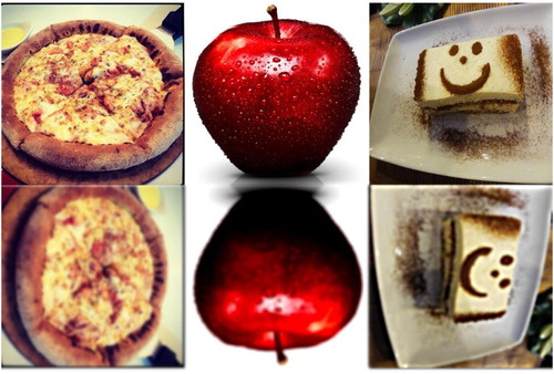
In this study, three different DCNN architectures and pre-trained models AlexNet and CaffeNet were trained on the extended version of Food11 dataset. In addition to the images of Food11 dataset, some images were randomly taken from the Food101 dataset. Transformations such as blurring, rotation were applied on some images that are randomly selected from each category. Gaussian blurring filter was applied to randomly selected image and then the image was rotated with randomly selected angle. Transformation was utilized for data augmentation. After augmented training dataset was obtained, images were resized to 512 × 512 and each image in the dataset was applied to the proposed and tested structures. Figure 3 shows samples from the dataset which are used as training data. The first row shows original images and the second row shows transformed images.

Figure 3. Samples from the dataset.

The main goal of the study is to propose an efficient DCNN architecture which is specific for food recognition. To achieve this aim, three structures which are similar to AlexNet were trained with different learning techniques, such as Adam, stochastic gradient descent and Nesterov accelerated gradient, and their performances were compared with that of pre-trained AlexNet and CaffeNet (BVLC-Alexnet; BVLC-CaffeNet). Transfer learning was applied to both models, while pre-trained weights were utilized for feature extraction parts, classifier part was trained with the same learning techniques utilized for proposed structures. The proposed structures are given in Table 1. For convolutional layers, filter size, stride, padding size, number of filters, activation function are given respectively. The maximum operator is utilized in pooling layers. For pooling layers, the first information is kernel size and the second one is stride. Fully connected layer size and activation functions are given respectively with FC label.

Table 1. Proposed structures.

Structure 1	Structure 2	Structure 3
Conv1: 7: 4: 0: 120: ReLU Max Pool:3:2 LRN	Conv1: 11: 4: 0: 96: ReLU Max Pool:3:2	Conv1: 7: 4: 0: 120: ReLU Max Pool:3:2
Conv2: 5: 1: 2: 240: ReLU Max Pool:3:2 LRN	Conv2: 5: 1: 2: 256: ReLU Max Pool: 3:2	Conv2: 5: 1: 2: 240: ReLU Max Pool:3:2
Conv3: 3: 1: 1: 360: ReLU	Conv3: 3: 1: 1: 384: ReLU	Conv3: 3: 1: 1: 360: ReLU
Conv4: 3: 1: 1: 360: ReLU	Conv4: 3: 1: 1: 384: ReLU Max Pool:3:2	Conv4: 3: 1: 1: 360: ReLU
Conv5: 3: 1: 1: 360: ReLU Max Pool:3:2	FC1: 4096: ReLU Dropout	Conv5: 3: 1: 1: 360: ReLU Max Pool:3:2
FC1: 500: ReLU Dropout	FC2: 4096: ReLU Dropout	FC1: 500: ReLU Dropout
FC2: 300: ReLU Dropout	FC3: Softmax	FC2: 300: ReLU Dropout
FC3: Softmax		FC3: Softmax

Although the first structure is very similar to AlexNet, however, it contains different kernel size and number of layers. The only difference between the first structure and the third one is that the third structure does not use a local response normalization layer. The idea behind this is to examine the effect of local response normalization layers. The second structure uses four convolutional layers followed by fully connected layers. Similar to the first structure and AlexNet, the pooling layer is not applied to third and fourth convolutional layers.

While these structures were trained from scratch, transfer learning was applied to AlexNet and CaffeNet structures. Pre-trained models were utilized as feature extractors and their classification parts were trained with the same learning techniques.

The first learning technique utilized in this study was stochastic gradient descent. In this technique, weights are updated after each training datum, as given in Equation (4) where is the weight matrix and is the learning rate (Goodfellow, Bengio, & Courville, 2016).

Let be the softmax result for jth datum’s correct result, loss function for j is the negative log likelihood for the correct result :(4) The main drawback of the stochastic gradient descent is its computational cost. Therefore to accumulate the learning momentum techniques were introduced (Goodfellow et al., 2016). Momentum techniques accelerate the movement by using past gradient changes. They use a velocity term to represent the past gradient effect. There exist different momentum techniques such as standard, Nesterov’s momentum, Adam which are given in Equations (5), (6) and (7), where is the momentum rate, are decay rates for moments and is a small constant, respectively (Goodfellow et al., 2016):(5) (6) (7)

Unlike standard momentum technique, Nesterov’s momentum calculates velocity before gradient calculation. Although it improves the convergence for batch learning, for stochastic gradient descent it does not improve convergence (Goodfellow et al., 2016).

On the other hand, the Adam technique is an adaptive learning rate optimization method. It uses first- and second-order moments (Goodfellow et al., 2016).

Test and results

Proposed architectures and pre-trained models were tested on the extend version of Food11 dataset with Nvidia Digit framework on NVIDIA GTX1070 GPU. Since weight and bias values were generated randomly, tests were carried out five times to eliminate randomness and Table 3 represents average accuracies. Total number of images in the dataset is 17,944. Train/Dev/Test distributions are 12,561, 2691 and 2692, respectively. Since dataset includes different sized images, they were resized to 512 × 512. Table 2 shows initial learning parameters used in the training phase.

Table 2. Learning parameters.

Parameters	Values
Learning rate	0.0001
Momentum	0.9
Maximum iteration	600 (Adam), 2000 (SGD), 600 (Nesterov’s)

Three different learning techniques and five different structures were compared, and their results are given in Table 3.

Table 3. Test results.

Model	Accuracy (%) (SGD)	Accuracy (%) (Nesterov’s accelerated gradient)	Accuracy (%) (Adam)
CaffeNet (BVLC-Caffenet)	80.51	81.55	83.7
AlexNet (BVLC-Alexnet)	82.07	83.01	86.92
Structure 1	70.12	71.55	73.80
Structure 2	38.85	47.63	71.7
Structure 3	53.78	68.55	69.92

According to the test results, while CaffeNet and AlexNet provided better classification performances with all learning techniques, proposed structures with Adam learning method provided acceptable results. Although both Nesterov’s acceleration and Adam technique improved the performances, it is clearly seen that the efficiency of the Adam technique is better than Nesterov’s technique. Especially, for stucture-2, the efficiency of the Adam technique is quite high. The limited contribution of Nesterov’s technique may be caused by the number of iterations. Classification performance with Nesterov’s technique can be improved by increasing the number of iterations. When structure-1 and structure-3 are compared, the advantage of local response normalization may be seen. The main advantage of local response normalization layer is to detect high-frequency features by normalizing the ReLU output.

Conclusion

In this study, the development of a pre-trained structure for food recognition was aimed. To achieve this aim, three different models were implemented, and their performances were compared with that of popular pre-trained models AlexNet and CaffeNet. The transfer learning technique was utilized to be able to use these pre-trained models for our problem. Three similar structures were proposed for analysing the effectiveness of layers separately. While the first structure includes local response normalization layers as in AlexNet and CaffeNet, the third structure is the same as the first structure except local response normalization. On the other hand, the second structure is similar to the third structure; however, it includes four convolutional layers and the number of filters utilized in convolutional layers and their filter sizes are also different. Moreover, different learning techniques were also applied for performance comparison. Since proposed models were trained from scratch, a large dataset was required. Hence, the Food11 dataset was extended with randomly chosen data from the Food101 dataset. Moreover, transformations such as blurring and rotation were applied. The balanced dataset was obtained by ensuring that at least 1500 images exist for each class.

Training and testing were implemented on NVIDIA Digit Framework with NVIDIA GTX1070. Each train and test processes for SGD took almost 1 day. On the other hand, for Adam and Nesterov’s technique, each train and test processes took almost 2.5 h. Test results show that pre-trained models provide better results than proposed models as expected. While the Adam technique improved classification performance maximally 32.85%, Nesterov’s improvement was maximally 14.77%.

Consequently, this study may be considered as the first step for developing a pre-trained model for food recognition. It also shows that the Adam learning technique improves the performance even if the structure is small and it requires fewer iterations. As future works, pre-trained food recognition structures with different classifiers are aimed.

Disclosure statement

No potential conflict of interest was reported by the authors.

ORCID

B. Melis Özyildirim http://orcid.org/0000-0003-1960-3787

Notes on contributors

Gözde Özsert Yiğit completed BSc and MSc in 2012 and 2016, and started her Phd in Computer Engineering Department of Cukurova University. She is working as research assistant in Computer Engineering department at Gaziantep University. Her research areas are artificial neural networks, deep learning.

B. Melis Özyildirim completed BSc, MSc in Computer Engineering Department of Cukurova University and completed Phd in 2015 in Electrical and Electronics Engineering Department of Cukurova University. She is working as assistant professor doctor in Computer Engineering Department of Cukurova University. Her research areas are machine learning, deep learning.

References

- BVLC-Alexnet. Retrieved from https://github.com/BVLC/caffe/tree/master/models/bvlc_alexnet
- BVLC-Caffenet. Retrieved from https://github.com/BVLC/caffe/tree/master/models/bvlc_reference_caffenet
- Chandrakumar, T., & Kathirvel, R. (2016). Classifying diabetic retinopathy using deep learning architecture. International Journal of Engineering Research & Technology (IJERT), 5(6), 19–24.
- Deng, J., Dong, W., Socher, R., Li, L. J., Li, K., & Li, F. (2009). Imagenet: A large-scale hierarchical image database. In IEEE Conference on Computer Vision and Pattern Recognition (CVPR 2009), 248 255.
- Ginzburg, B. (2014). Deep learning summer workshop”, Ver. 06. Retrieved from http://courses.cs.tau.ac.il/Caffe_workshop/Bootcamp/pdf_lectures/Lecture%202%20Caffe%20-%20getting%20started.pdf
- Goodfellow, I., Bengio, Y., & Courville, A. (2016). Deep learning. Cambridge: MIT Press.
- International Diabetes Federation. (2016). Update 2015, 13.
- Karnowski, J. (2015). AlexNet + SVM. Retrieved from https://jeremykarnowski.files.wordpress.com/2015/07/alexnet2.png
- Kawano, Y., & Yanai, K. (2014). Food image recognition with deep convolutional features. ACM UbiComp workshop on cooking and eating activities.
- Kawano, Y., & Yanai, K. (2015). Foodcam: A real time food recognition system on a smartphone. Multimedia Tools and Applications, 74(14), 5263–5287. doi: 10.1007/s11042-014-2000-8
- Krizhevsky, A., Sutskever, I., & Hinton, G. (2012). ImageNet classification with deep convolutional neural networks. NIPS'12 Proceedings of the 25th international conference on neural information processing systems, 1, 1097–1105.
- LeCun, Y., Bottou, L., Bengio, Y., & Haffner, P. (1998). Gradient based learning applied to document recognition. In Proceedings of the IEEE, pp. 2278–2324.
- Liu, C., Cao, Y., Luo, Y., Chen, G., Vokkarane, V., & Ma, Y. (2016). DeepFood: Deep learning-based food image recognition for computer-aided dietary assessment. ICOST 2016, International conference on smart homes and health telematics, vol. 9677, 37–48.
- The Ministry Health of Turkey, Public health Institution. 2017. The department of obesity, diabetes and metabolic diseases. Accessed 10 March 2017.
- Nielsen, M. A. (2015). Neural networks and deep learning. Determination Press.
- Ravi, D., Wong, C., Deligianni, F., Berthelot, M., Andreu-Perez, J., Lo, B., & Yang, G. (2017). Deep learning for health informatics. IEEE Journal of Biomedical and Health Informatics, 21(1), 4–21. doi: 10.1109/JBHI.2016.2636665
- Sankar, M., Batri, K., & Partvathi, R. (2016). Earliest diabetic retinopathy classification using deep convolution neural networks. International Journal of Advanced Engineering Technology, 2(1), 460–470.
- Sermanet, P., Eigen, D., Zhang, X., Mathieu, M., Fergus, R., & LeCun, Y. (2013). Overfeat: Integrated recognition, localization and detection using convolutional networks. arXiv Preprint, arXiv, 1312–6229.
- Single, A., Yuan, L., & Ebrahimi, T. (2016). Food/non-food image classification and food categorization using pre-trained GoogLeNet model. Proceedings of the 2nd international workshop on multimedia assisted dietary management (MADIMA 2016), 3–11, 16.
- Szegedy, C., Liu, W., Jia, Y., Sermanet, P., Reed, S., Anguelov, D., … Rabinovich, A. (2015). Going deeper with convolutions. In 2015 IEEE conference on computer vision and pattern recognition (CVPR), 1–9.
- Tennakoon, R., Mahapatra, D., Ro, P., Sedai, S., & Garnavi, R. (2016). Image quality classification for DR screening using convolutional neural networks. In Proceedings of the ophthalmic medical image analysis international workshop.
- Trivedi, A. (2016). Deep learning part 2: Transfer learning and fine-tuning deep convolutional neural networks. Retrieved from http://blog.revolutionanalytics.com/2016/08/deep-learning-part-2.html
- Vos, T., Flaxman, A. D., Naghavi, M., Lozano, R., Michaud, C., Ezzati, M., Shibuya, K., Salomon, J. A., Abdalla, S., Aboyans, V., et al. (2012). Years lived with disability (YLDs) for 1160 sequelae of 289 diseases and injuries 1990–2010: A systematic analysis for the global burden of disease study 2010. The Lancet, 380(9859), 2163–2196. doi: 10.1016/S0140-6736(12)61729-2
- World Health Organization. (2014). About diabetes. Archived from the original on 31 March 2014. Retrieved 4 April 2014.
- Yanai, K., & Kawano, Y. (2015). Food image recognition using deep convolutional network with pre-training and fine-tuning. IEEE international conference on multimedia & expo workshops (ICMEW).
- Yigit, O. G., & Ozyildirim, B. M. (2017). Comparison of convolutional neural network models for food image classification. 2017 IEEE International Conference on INnovations in Intelligent SysTems and Applications (INISTA), Gdynia, 2017, pp. 349–353.