Speech feature extraction using linear Chirplet transform and its applications*

ABSTRACT

Most speech processing models begin with feature extraction and then pass the feature vector to the primary processing model. The solution's performance mainly depends on the quality of the feature representation and the model architecture. Much research focuses on designing robust deep network architecture and ignoring feature representation's important role during the deep neural network era. This work aims to exploit a new approach to design a speech signal representation in the time-frequency domain via Linear Chirplet Transform (LCT). The proposed method provides a feature vector sensitive to the frequency change inside human speech with a solid mathematical foundation. This is a potential direction for many applications. The experimental results show the improvement of the feature based on LCT compared to MFCC or Fourier Transform. In both speaker gender recognition, dialect recognition, and speech recognition, LCT significantly improved compared with MFCC and other features. This result also implies that the feature based on LCT is independent of language, so it can be used in various applications.

KEYWORDS:

• speech representation
• time-frequency domain
• linear chirplet transform
• instantaneous frequency
• speech processing

1. Introduction

During the development of the speech processing field, many methods for speech representation are proposed. A wide range of applications, from speech recognition, speaker authentication, and emotion recognition, use many forms of speech representation as the input for the model. The methods for representing human speech were mainly researched and designed long ago and have not been a hot topic since 2010. Many states of the art models in speech processing are mainly based on the deep learning approach, which requests many data for training and powerful computing resources. Our main question in this research is how to design a more meaningful form for speech representation to loosen the data and compute resource requirements.

In the past, many feature extraction approaches were proposed to represent human speech in new spaces, which are easier to solve speech-related recognition problems. There are two groups with the root ideas to design the representation space. The first group of speech signal features relates to stationary analysis, while the second one uses the strength of a deep neural network to model the feature space.

The first group originates from the phenomenon that the vibration of two vocal tracks creates human speech. This fact shows that speech signals can be seen as stationary signals. So most acoustics properties, including content, prosody, and emotion, can be analyzed in the frequency domain. On the other hand, this stationary nature of speech signals impacts many hierarchical levels of spoken languages, such as phonemes, words, phrases, or whole sentences. In this group, the earlier sub-group with stationary features includes the pitch or frequency $f_0$, energy, and duration of the signal (Cowie & Douglas-Cowie, 1996). These features reflect the speech behaviors merely in a less meaningful space. The second sub-group includes many methods that use the integral transform to represent the data in a new space with a more informative form. Some representatives in this group can be listed as Fourier Transform, Wavelet Transform, and their extensions (Koolagudi & Rao, 2012).

Integral transforms use a new space named the frequency domain, or spectrum space, to present the speech feature. Because of speech creation, the signal is nearly stationary, which is analyzed effectively in the frequency domain. Analyzing the speech in this domain emphasizes the process of modeling and exploiting the speech data. Conventional transforms, such as Fourier Transform, can be applied first to convert the speech into the spectrum. Then many post-processing techniques are proposed, including Mel Frequency Cepstral Coefficients (MFCC) (Koolagudi & Rao, 2012), Envelope Subtraction (Do et al., 2021), Linear Prediction Cepstral Coefficients (LPCC), Log-Frequency Power Coefficients (LFPC), or Gammatone Frequency Cepstral Coefficients (GFCC) (Nwe et al., 2003). These features are the more robust forms of the spectrum with some differences in design. Each is established to emphasize other aspects of a speech signal, corresponding with different applications.

The second group uses a deep neural network such as AutoEncoder (Do et al., 2020a), which receives raw speech signal and then propagates to reach the final result (Tzirakis et al., 2018). In this approach, the feature vector with its pure meaning does not exist (Do et al., 2020b, 2020c). A deep neural network is a black box, so no pure algorithm for speech feature vectors is implemented. On the other hand, all layers in the network can also be seen as feature vectors with different meaningful levels. Although its meaning is unclear, hidden layers in neural networks positively improve the whole model's performance. The reason is that a neural network can extract the idiosyncratic vector in a hidden space. Although the feature is not visible in our observable space, it is separable in the latent space. Because the model's output comes from the computing process in these latent spaces, separation ability in the hidden space yields good results.

The two groups below include many advantages and also disadvantages. This motivates us to design a new feature to strengthen the feature vector in particular cases. The first group exploits the periodic features, while the second group uses the power of a deep neural network. We aim to establish a more meaning-richer feature extraction algorithm than the first group and more apparent and interpretable than the second group.

Many applications, including speaker authentication, gender recognition, emotion recognition, dialect recognition, etc. relate to the trend and change in speech frequency. The values of $f_0$, energy, silence, or spectrum and its extensions concentrate on the aspect stationary of speech, so they must be better for the recognition tasks mentioned above. While speech recognition needs the stationary of the signal to form the phoneme, emotion or dialect is defined based on the change during the pronunciation process. Traditional Fourier Transform and their variances can show the signal properties in the statics frequency domain. The coefficients of their representation reflect the contribution of each particular frequency element to the whole signal. We need a better design to gain a better feature vector encoding the signal change.

Linear Chirplet Transform (LCT), proposed at the same time by Mann and Haykin (1991), Mann and Haykin (1995), and Mihovilovic and Bracewell (1991), provides a fundamental method to exploit the change in the general signal, including human speech. Chirplet is a piece of chirp, a signal with a frequency that increases or decreases. LCT can become a potential approach for speech representation related to many applications requiring frequency change from its idea and origin. Compared with conventional Fourier Transform, LCT models the signal more flexibly. While Fourier Transform uses the basis vector set with a fixed instantaneous frequency, LCT builds a basis vector set with a time-linear function for instantaneous frequency. This linear function can be described with a new parameter called chirp rate. With this parameter, the transform can emphasize every grade of change in frequency during the time.

Within this research, what we contribute includes these aspects:

• Explaining the limit of traditional spectrum using Fourier Transform in many applications relating to speech frequency change.

• Designing a new algorithm via LCT operator for speech representation to emphasize the frequency change in the human speech signal.

• Proving the advantages of the proposed feature experimentally via three tasks, including speaker gender recognition, speaker dialect recognition, and speech recognition.

The remaining of this paper is organized as follows. Section 2 briefly introduces the LCT. We present the linear form of this transform because this approach is the most suitable choice for the case in which the signal is modeled as a linear chirp. Section 3 applies LCT into speech processing. This section presents this research's most important contribution: an algorithm for speech feature extraction using LCT. Section 4 shows the experiments in speech processing. We validated our proposed algorithm using LCT and compared it with some commonly used methods. Experimental results show that LCT is a potential approach for speech feature extraction. Then Section 5 discusses some central aspects of the LCT for speech processing. Finally, the paper ends with the section of summary and conclusion.

2. Linear Chirplet transform

The LCT was first introduced in 1991 by Mann and Haykin (1991) and Mihovilovic and Bracewell (1991) to model the chirp signal. With signal $s(t)\in L^2(R)$, in the first step, its analytical form is established using Hilbert transform (Liu et al., 2020) as follows: (1) $z(t)=s(t)+j\mathcal{H}[s(t)]$(1) with $\mathcal{H}$ denotes Hilbert transform. This process is used to remove all negative frequency components in the signal. Next, the original form of LCT is defined as: (2) $C{T}_s(t_0,\omega ,\alpha ,\sigma )={\int }_{-\mathrm{\infty }}^{+\mathrm{\infty }}z(t){\mathrm{\Psi }}_{t_0,\alpha ,\sigma }^{\ast }(t)\exp (-j\omega t)\mathrm{d}t$(2) with ${\mathrm{\Psi }}_{t_0,\alpha ,\sigma }^{\ast }$ is the complex window described by: (3) ${\mathrm{\Psi }}_{t_0,\alpha ,\sigma }(t)=w_{(\sigma )}(t-t_0)\exp (-j\frac{\alpha }{2}{(t-t_0)}^2)$(3) In the Equation (3(3) ${\mathrm{\Psi }}_{t_0,\alpha ,\sigma }(t)=w_{(\sigma )}(t-t_0)\exp (-j\frac{\alpha }{2}{(t-t_0)}^2)$(3) ), $t_0$ denotes time, the real number α denotes chirp rate, and w denotes the window function with parameter σ. The chirp rate α is one of the most important parameters used to control the slope of the basis vector in the time-frequency plane.

The window $w\in L^2(R)$ is a normalized real window, which identifies and normalizes the range in the signal used to compute the coefficients. Normally, the Gaussian function, one of the most common choices for the window, is defined as: (4) $w_{(\sigma )}(t)=\frac{1}{\sqrt{2\pi }\sigma }\exp (-\frac{1}{2}{\left(\frac{t}{\sigma }\right)}^2)$(4) with σ as the standard deviation for the Gaussian function.

With the original form in the Equation (2(2) $C{T}_s(t_0,\omega ,\alpha ,\sigma )={\int }_{-\mathrm{\infty }}^{+\mathrm{\infty }}z(t){\mathrm{\Psi }}_{t_0,\alpha ,\sigma }^{\ast }(t)\exp (-j\omega t)\mathrm{d}t$(2) ), it is difficult to compute the transform result. This leads the LCT to be interpreted as an extension of the Short Time Fourier Transform (STFT) of the analytical signal. So the Equation (2(2) $C{T}_s(t_0,\omega ,\alpha ,\sigma )={\int }_{-\mathrm{\infty }}^{+\mathrm{\infty }}z(t){\mathrm{\Psi }}_{t_0,\alpha ,\sigma }^{\ast }(t)\exp (-j\omega t)\mathrm{d}t$(2) ) can be re-written as: (5) $C{T}_s(t_0,\omega ,\alpha ,\sigma )=A(t_0){\int }_{-\mathrm{\infty }}^{+\mathrm{\infty }}\overline{z}(t)w_{(\sigma )}(t-t_0)\exp (-j\omega t)\mathrm{d}t$(5) with: (6) $\overline{z}(t)=z(t){\mathrm{\Phi }}_{\alpha }^R(t){\mathrm{\Phi }}_{\alpha }^M(t,t_0)$(6)

Function ${\mathrm{\Phi }}_{\alpha }^R(t)$ presents for frequency operator in the time-frequency plane: (7) ${\mathrm{\Phi }}_{\alpha }^R(t)=\exp (-j\alpha \frac{t^2}{2})$(7) This operator rotates the analytical signal $z(t)$ by θ. This angle satisfies the constraint that $\theta =Acrtan(-\alpha )$.

Function ${\mathrm{\Phi }}_{\alpha }^M(t,t_0)$ is the shifting operator. It relocates the frequency component from ω to $\omega +\alpha t_0$: (8) ${\mathrm{\Phi }}_{\alpha }^M(t,t_0)=\exp (j\alpha t_{0}t)$(8) The analytical signal can be transformed via LCT using STFT as the fundamental technique with the rotating and shifting operators above.

The remaining factor in the Equation (5(5) $C{T}_s(t_0,\omega ,\alpha ,\sigma )=A(t_0){\int }_{-\mathrm{\infty }}^{+\mathrm{\infty }}\overline{z}(t)w_{(\sigma )}(t-t_0)\exp (-j\omega t)\mathrm{d}t$(5) ) is the amplitude, which is defined by: (9) $A(t_0)=\exp (-j{t}^2\frac{\alpha }{2})$(9) To simplify the computing process, because the amplitude has the modulus $|A(t_0)|=1$, it should be removed from the Equation (5(5) $C{T}_s(t_0,\omega ,\alpha ,\sigma )=A(t_0){\int }_{-\mathrm{\infty }}^{+\mathrm{\infty }}\overline{z}(t)w_{(\sigma )}(t-t_0)\exp (-j\omega t)\mathrm{d}t$(5) ). So the final form for the LCT is described by: (10) $C{T}_s(t_0,\omega ,\alpha ,\sigma )={\int }_{-\mathrm{\infty }}^{+\mathrm{\infty }}\overline{z}(t)w_{(\sigma )}(t-t_0)\exp (-j\omega t)\mathrm{d}t$(10) From these analyses, there are three main stages to implement the LCT as follows:

• Step $\mathrm{\#}$1: Rotating the analytical signal by the angle $\theta =Arctan(\alpha )$.

• Step $\mathrm{\#}$2: Shifting the output of step $\mathrm{\#}$1 with an increment of $\alpha t_0$ in the direction of frequency.

• Step $\mathrm{\#}$3: Applying STFT with the signal received after step $\mathrm{\#}$2, with Gaussian window $w_{(\sigma )}$.

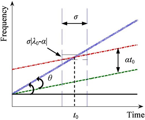
These three steps are illustrated in the Figure 1 (Yang et al., 2014). Assuming the objective signal has the instantaneous frequency trajectory as the blue line, which is identified as: (11) $\omega ={\omega }_0+{\lambda }_{0}t$(11) This function is purely linear or the simplest function to represent the trajectory for instantaneous frequency. After step $\mathrm{\#}$1, the signal rotates and becomes the green line. As in the Figure 1, the rotating angle is θ, which is defined by $\theta =Arctan(-\alpha )$. Next, the signal is increased with a distance $\alpha t_0$ in the direction of frequency and returns the red line. Finally, the red signal is normalized with a Gaussian window and then passed into STFT to compute the coefficient corresponding with time $t_0$ and frequency ω.

Figure 1. Illustration of the Linear Chirplet Transform with three main steps. In step $\mathrm{\#}$1, the blue line is rotated by an angle θ, then becomes the green line. In step $\mathrm{\#}$2, the green line is shifted by $\alpha t_0$ to be the red line. At the final step, the red line is transformed with STFT.

3. Speech representation with linear Chirplet transform

3.1. The difference between linear Chirplet transform and short-time fourier transform

Linear Chirplet Transform and Fourier Transform share the same idea about converting the signal from the time domain into another domain. While Fourier Transform uses the basis vector with a fixed frequency, LCT processes the input signal with a dynamic-frequency basis vector. In the time-frequency plane, the basis vectors used in Fourier Transform are presented as horizontal lines and are difficult to modify. On the other hand, the LCT provides the parameter called chirp rate α to control the slope of the instantaneous frequency trajectory. In a particular problem, with a particular type of data, the parameter of LCT can be adjusted flexibly to capture meaningful information from data.

To illustrate the difference between LCT and Fourier Transform, let us consider a signal component signal as follow: (12) $s(t)=\sin \left(2\pi (10t+\frac{5}{4}{t}^2+\frac{1}{9}{t}^3-\frac{1}{160}{t}^4)\right)$(12) So, using the FM model, we receive the instantaneous phase: (13) $\varphi (t)=10t+\frac{5}{4}{t}^2+\frac{1}{9}{t}^3-\frac{1}{160}{t}^4$(13) and then the objective instantaneous frequency is: (14) $\omega ={\varphi }^{\prime }(t)=10+\frac{10}{4}t+\frac{1}{3}{t}^2-\frac{1}{40}{t}^3$(14)

Figures 2 and 3 show the instantaneous frequency trajectories returned by Linear Chirplet Transform with different chirp rates. Figure 2 presents the trajectory with $\alpha =0$, corresponding with Fourier Transform. On the other hand, Figure 3 shows the trajectory with a chirp rate $\alpha >0$. These illustrations mean that Fourier Transform is a special case of LCT with zero chirp rate. Moreover, LCT can transform in many directions with the flexibility of α.

Figure 2. Linear Chirplet Transform with chirp rate $\alpha =0$. In this case, LCT performs equivalent with the Fourier transform.

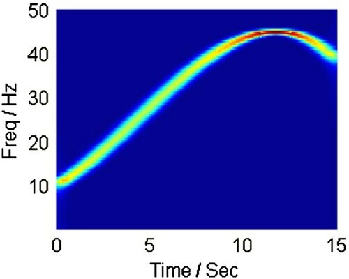
Figure 3. Linear Chirplet Transform with positive chirp rate $\alpha =5$. In the TF plane, the signal is highlighted with red color when the frequency achieving high energy increases over time.

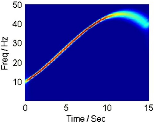
The figures above clearly show the properties of two transforms, LCT and Fourier Transform:

• Both of LCT and Fourier Transform: estimating the main trajectory of the signal in the time-frequency plane correctly

• Fourier Transform: focusing on the plane's stable area or the signal's stationary properties. In Figure 2, the value at the top of the curve is red color, presenting big values, while the remaining in the curve is green color, meaning smaller values.

• LCT with positive chirp rate (see Figure 3): mainly painted red color, emphasizing the range with a significant increase. The other ranges in the curve, stable or decreasing, are not highlighted and painted green.

3.2. Feature design for speech using the linear Chirplet transform

Algorithm 1. Speech feature extraction using Linear Chirplet Transform

1. procedure Feature-Extraction($T,\mathrm{\Omega },\alpha ,\sigma ,s(t)$)

2. $z(t)\leftarrow s(t)+j\mathcal{H}[s(t)]$

3. $Feature\leftarrow [,]$

4. for $t_0\in T$ do

5.  for $\omega \in \mathrm{\Omega }$ do

6.   $z_{t_0,\omega }(t)\leftarrow z(t)w_{(\sigma )}(t-t_0)$

7.   $z_{t_0,\omega }^R(t)\leftarrow z_{t_0,\omega }(t){\mathrm{\Phi }}_{\alpha }^R(t)$

8.   $z_{t_0,\omega }^{R,M}(t)\leftarrow z_{t_0,\omega }^R(t){\mathrm{\Phi }}_{\alpha }^M(t,t_0)$

9.   $Feature[t_0,\omega ]\leftarrow {\int }_{-\mathrm{\infty }}^{+\mathrm{\infty }}{z}_{t_0,\omega }^{R,M}(t)\exp (-j\omega t)\mathrm{d}t$

10.  return Feature

Algorithm 1 extracts the speech feature via two important stages: defining the hyperparameters and running the transform to get the feature representation. The hyperparameters for LCT include:

• T: a set of time points for the features. In practice, one second of a signal with a sample rate of $16000\mathrm{Hz}$ is usually divided to get 40 time points. Each time point corresponds with 400 samples in the time domain.

• Ω: a set of frequency. In range $[1\mathrm{Hz},8000\mathrm{Hz}]$ or $[1\mathrm{Hz},16000\mathrm{Hz}]$, Ω usually contains 256 or 512 values.

• α: chirp rate

• σ: standard deviation of the Gaussian window

After defining the hyperparameters, the feature extraction stage is processed as in the Algorithm 1 with $w_{(\sigma )}(t)$, ${\mathrm{\Phi }}_{\alpha }^R(t)$, and ${\mathrm{\Phi }}_{\alpha }^M(t,t_0)$ are defined in Section 2.

Algorithm 1 is sensitive to the frequency change in the speech signal. If the chirp rate $\alpha >0$, this method can capture so well the moment that the speech tone increases. Figure 4 shows a 3D illustration of a speech signal after processing by our proposed algorithm.

Figure 4. Illustration of 3D time-frequency representation returned by Linear Chirplet Transform for input audio with the content ‘There was a change now’, said a woman.

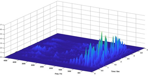
In Figure 4, the valuable information concentrates mainly on the frequency range $[50\mathrm{Hz},1200\mathrm{Hz}]$, or human voice band. The top coefficients, highlighted with yellow and green, occur sparsely in the representation. In this speech signal, the female speaker increases her tone significantly at these positions. This information could become the key for identification or recognition tasks.

4. Experiment

This section evaluates the proposed method and compares it with conventional features. Mainly, we apply the LCT method as the feature extractor for speaker gender recognition, speaker dialect recognition, and speech recognition. We use the state-of-the-art model with different features, including spectrum, Mel-spectrum, MFCC, and the proposed method with each task. The experimental detail will be presented in the following sub-sections.

4.1. Problems and datasets

4.1.1. Speaker gender recognition

The first experiment is speaker gender recognition. Gender, in a dialogue or communication, is not essential in some languages but is very important in other languages. This depends on the organization of personal pronouns in each language. For many applications, such as virtual assistants or automatic call centers, to know the gender of a customer for smooth communication, the system needs to know the speaker's gender.

Gender recognition is a simple binary classification identifying whether a voice is male or female. This problem is described by: (15) $(input,output)=(speech\mathrm{\_}signal,label)$(15) with label = m for man, and label = f for woman. We use TIMIT (Fisher, 1986) and VIVOS (Luong & Vu, 2016) for English and Vietnamese for this task, respectively. These two datasets, in terms of gender, hold the data as in Table 1.

Table 1. Some statistics in TIMIT and VIVOS.

Information	TIMIT	VIVOS
Male (recorders)	438	34
Female (recorders)	192	31
Total recorders	630	65
Total dialects	8	3
Total audio files	6300	12420
Total length (hours)	5.4	15.7

4.1.2. Speaker dialect recognition

Speaker dialect provides much helpful information for content providers. In many applications, from the speaker dialect, the systems can know or predict the customer's hometown and national/regional culture, then suggest suitable content or advertisements. On the other hand, many connection services or dating applications can make better suggestions with the users' dialect.

Like gender recognition, speaker dialect recognition is formulated as a classification problem. The difference is that the number of classes is higher than the gender classification. In TIMIT, there are eight different dialects, while in VIVOS, this number is three dialects. This problem, in terms of data, is more complicated than gender recognition. While each gender is clear and different enough for the classifier to know which gender it is, dialect is not straightforward. Because a person can change the accommodation, keep moving during life as a global citizen, or work in an international company, there is no natural dialect thereof. Identifying a person's dialect takes work, even with an adult. This becomes a more difficult task for the proposed method.

We use TIMIT and VIVOS for learning and testing models in this task. While TIMIT contains eight dialects including New England, Northern, North Mid- land, South Midland, Southern, New York City, Western, and Army Brat; VIVOS only contains three main dialects in Vietnamese: North, Central, and South. These two datasets are small but contain enough information for model learning. On the other hand, they also contain the most common dialects in both English and Vietnamese. This ensures that the experimental results distribute similarly to real life.

4.1.3. Speech recognition

Speech recognition is much more complicated than the two previous problems. This task's primary mission is to translate the original human speech into text. Speech recognition is the first step of any system interacting with people using the human voice. In virtual assistants, smart homes, smart cars, or robotics, the users can interact with the system by talking directly. In these systems, the first sub-system is speech recognition, receiving the human voice, translating it into text, and passing it to the other module for language understanding. The systems above can still work without speech recognition but are much more difficult.

Speech recognition is arduous because the input signal usually contains noise, or the data could be more stable. One person talks the same content twice, but the recorded audios differ. There is no way to deal with speech recognition without an effective method.

This recognition problem is modeled as a sequence tagging task, whose input and output are defined by: (16) $(input,output)=(speech\mathrm{\_}signal,text)$(16) When the input speech signal is separated into frames, the problem becomes: (17) $(input,output)=(f_0{f}_1{f}_2\dots f_n,c_0{c}_1\dots c_m)$(17) with $f_i$ denotes the ith frame, and $c_j$ is the jth character. In this task, the amount of frame n and the number of characters m are usually different because human speech contains many walls of silence that are not written.

To train the model on recognizing human speech, we still use VIVOS for Vietnamese, but the dataset for English is LibriSpeech (Panayotov et al., 2015). Because the input and output lengths are much longer than classes for speaker gender and dialect, we need to use a larger dataset for the learning process. In Vietnamese, VIVOS is the best dataset regarding audio quality and the covering ability of vocabulary and phoneme sets. We continue using this dataset even though its length is insufficient for a speech recognition model. With LibriSpeech, the total audio length is improved significantly, as shown in Table 2.

Table 2. Some statistics in LibriSpeech.

Information	Amount
Male (recorders)	1210
Female (recorders)	1128
Total recorders	2338
Dialects	Not mention
Total length (hours)	960
# words	977.000

4.2. Experimental designs

4.2.1. Speaker gender and dialect recognition

In both speaker gender and dialect recognition, we split and pre-process audio data similarly. Particularly, we do some steps as follows:

• We split speech signals into chunks of 1 second.

• Two consecutive chunks overlap $25\mathrm{ms}$.

• The label for each chunk is taken from the label of the original audio.

• Re-format each data point for leaning into: (18) $data\mathrm{\_}point=(input,output)=(chunk,label)$(18)

The input signals for gender and dialect recognition are the same, while the outputs differ based on the task.

To perform the primary processing phase, we use the simple CNN network Lenet (LeCun et al., 1989). This network includes five convolution layers followed by five pooling layers. Then the network connects to five fully connected layers. This is a simple CNN architecture, but it still works well with classification tasks, especially when the number of classes is meager, as in gender or dialect recognition.

We use the available separation for training and testing in TIMIT and VIVOS. In the training set, we split with the ratio 90:10 for training and validating. For each task, we train the models 20 epochs in a computer with 4GB RAM, CPU Core i5 4GHz to gain the results, shown in the Sub-section 4.3.

4.2.2. Speech recognition

In this task, we use two current state-of-the-art models to learn and process data: Transformer-Conformer (T-C) (Gulati et al., 2020) and Transducer (Jaitly et al., 2016). These models are very complicated, with many different layers and connections inside. We do not use the language model as the supporter or post-processing step to compare the speech feature representation only. The results reported in this paper are achieved when the input is only the speech signal.

With LibriSpeech for English and VIVOS for Vietnamese, we still use the available separation for training and testing. We use the ratio 90:10 for training:validating phases in the training set. Each model is trained with 50 epochs using a computer with 32GB RAM, CPU Core i5 4GHz, and 1xGPU Geforce RTX 3090, to gain good results, presented in the Sub-section 4.3.

4.2.3. Evaluation metrics

To evaluate the performances of the recognition models with many different extraction methods, we apply error rate and $f_1$ score for gender and dialect recognition. These two measures are usually used in classification problems as the standard method. The error rate is defined by: (19) $Error\mathrm{\_}Rate=\frac{\mathrm{\#}False\mathrm{\_}Prediction\mathrm{\_}Samples}{\mathrm{\#}Samples}$(19) The $f_1$ score is the harmonic mean of precision and recall, which is identified by: (20) $f_1\mathrm{\_}Score=\frac{2\mathrm{\#}True\mathrm{\_}Positive}{2\mathrm{\#}True\mathrm{\_}Positive+False\mathrm{\_}Positive+False\mathrm{\_}Negative}$(20) All terms in Equation (20(20) $f_1\mathrm{\_}Score=\frac{2\mathrm{\#}True\mathrm{\_}Positive}{2\mathrm{\#}True\mathrm{\_}Positive+False\mathrm{\_}Positive+False\mathrm{\_}Negative}$(20) ) only have their meaning with a particular classes, so $f_1$ score only has its meaning in an identified class. The scores reported in the Tables 3 and 4 are the average scores of the classes in the applications.

Table 3. Speaker gender recognition in TIMIT and VIVOS.

Feature	TIMIT	TIMIT	VIVOS	VIVOS
	Error_Rate(%)	$f_1$_ Score	Error_Rate(%)	$f_1$_ Score
Spectrogram	7.59	93.34	5.99	94.23
Mel-Spectrogram	8.62	93.02	3.51	96.55
MFCC	5.10	95.29	3.61	96.25
LCT ($\alpha =0.5$)	4.44	95.87	2.72	97.36
LCT ($\alpha =-0.5$)	4.39	95.89	2.52	97.42

Table 4. Speaker dialect recognition in TIMIT and VIVOS.

Feature	TIMIT	TIMIT	VIVOS	VIVOS
	Error_Rate(%)	$f_1$_ Score	Error_Rate(%)	$f_1$_ Score
Spectrogram	4.50	95.28	5.85	94.42
Mel-Spectrogram	4.21	95.52	4.10	95.86
MFCC	2.17	97.82	2.66	97.18
LCT ($\alpha =0.5$)	2.01	97.98	2.68	97.15
LCT ($\alpha =-0.5$)	1.95	98.02	2.69	97.37

To evaluate the effectiveness of different features in the speech recognition task, we apply Word Error Rate (WER) measure, which is: (21) $WER=\frac{\mathrm{\#}Substitutions+\mathrm{\#}Deletions+\mathrm{\#}Insertions}{\mathrm{\#}Words}$(21)

While $f_1$ score is as high as good, both $Error\mathrm{\_}Rate$ and WER are as low as good. This leads to the optimal feature yielding the maximum $f_1$ score and the minimum for $Error\mathrm{\_}Rate$ and WER, depending on the tasks.

4.3. Experimental results

4.3.1. Speaker gender recognition

Table 3 shows the result for the gender recognition task with many features. As can be seen in the table, the two lowest error rates are from LCT for both TIMIT and VIVOS. With $4.39\text{\%}$ and $2.52\text{\%}$ for these two datasets, LCT with negative chirp rate $\alpha =-0.5$ becomes the best choice for feature representation in this task. Compared with the following error rate from MFCC, the proposed method improves $0.71\text{\%}$ for TIMIT and $1.09\text{\%}$ for VIVOS. These numbers are significant.

Similar to the error rate, the $f_1$ score yields the best performances belonging to LCT with the negative chirp rate. The highest scores for TIMIT and VIVOS are $95.89\text{\%}$ and $97.42\text{\%}$, respectively. Although the difference between LCT with a positive chirp rate and LCT with a negative chirp rate is too small, the improvement of LCT compared with MFCC and other methods is observable.

4.3.2. Speaker dialect recognition

Table 4 shows error rates for the speaker dialect recognition task. Different from gender recognition, in this task, the best result is not always the proposed LCT. Particularly, LCT with a negative chirp rate gains the lowest error rate of $1.95\text{\%}$ for TIMIT, while MFCC yields the best result with an error rate of $2.66\text{\%}$ for VIVOS.

In this case, there are some different results between TIMIT and VIVOS. This could come from the difference in language or the dataset size. Although not get the best error rate for VIVOS, two LCT configurations perform similarly with the best result from MFCC: $2.66\text{\%}$ compared with $2.69\text{\%}$.

With $f_0$ score, the improvement of LCT compared with other features, especially with the negative α, is clear. Achieving $98.02\text{\%}$ and $97.37\text{\%}$ in TIMIT and VIVOS, LCT with $\alpha =-0.5$ gains the highest scores. These positive results imply that LCT could be used for dialect recognition in real applications.

4.3.3. Speech recognition

In Table 5, the reported results are identical to dialect recognition. The proposed LCT with a negative chirp rate becomes the best option for Transformer-Conformer in both English and Vietnamese with $6.29\text{\%}$ and $22.52\text{\%}$ in terms of WER. These results are slightly better than the traditional MFCC.

Table 5. Speech recognition with different features for English (E) in LibriSpeech and Vietnamese (V) in VIVOS.

Feature	T-C (E)	Transducer (E)	T-C (V)	Transducer (V)
	WER(%)	WER(%)	WER(%)	WER(%)
Spectrogram	8.65	8.02	25.87	34.65
Mel-Spectrogram	7.09	8.11	26.14	33.26
MFCC	6.47	6.45	23.73	28.08
LCT ($\alpha =0.5$)	6.38	6.47	23.91	29.28
LCT ($\alpha =-0.5$)	6.29	6.76	22.52	28.10

With the Transducer network, the lowest WER belongs to MFCC. In English, the LCT with a positive chirp rate returns the result approximating the best case, while LCT with a negative chirp rate gains the error rate $28.10\text{\%}$, only higher $0.02\text{\%}$ in comparison with the best result from MFCC.

5. Discussion and future works

Via three experiments, the proposed method, LCT, is always one of the best choices for all three tasks in English and Vietnamese. In speaker dialect recognition and speech recognition, LCT performs so well with very low error rates, but the improvement is not good, especially compared with MFCC. The difference between LCT and MFCC in these cases must be clarified, and the numerical results are similar. However, in the speaker gender recognition, LCT is more outstanding than the other methods, including MFCC. Both types of chirp rates show meager error rates, and the improvements are too clear compared with the remaining features.

The results yielded by LCT with negative and positive chirp rates are similar in the three cases, but the negative chirp rate is slightly better. This observation implies that both chirp rates are true and usable, or LCT is a potential approach, but LCT with a negative chirp rate could be better and become the optimal choice.

Back to the idea of LCT, this transformation aims to detect and reveal where the signal change in the time-frequency domain. LCT with a positive chirp rate filters where a voice increases the tone, while the negative chirp rate corresponds with where the voice decreases the tone. This also means that LCT is only good and outperforms tasks requiring data changes. Speech recognition and dialect recognition are the tasks requiring the stable in the input signal. When we listen to a normal voice, it is easy to know what the speaker says and the corresponding dialect. Nevertheless, it is more difficult to understand the content or dialect when the speaker keeps increasing or decreasing the tone. On the other hand, in gender recognition, with a more sensitive-change feature, the model can easily predict whether the speaker is male or female.

Via three experiments, the proposed LCT for speech feature extraction performs better than some widely used features such as MFCC or mel-spectrogram. Inspire positive results; the improvements are not significant. In our viewpoint, with a more complicated situation, such as emotion recognition, mixed dialects recognition, or age prediction, LCT could not perform well.

After 2010, there are two extensions of LCT, named Polynomial chirplet transform (Peng et al., 2011) and General linear chirplet transform (Yu & Zhou, 2016). We are planning to apply these transforms to establish new speech feature extractions. These transform can capture many hidden human speech behaviors, so we hope the extracted features work well in cases of mixed dialect recognition or emotion recognition.

6. Summary and conclusion

This paper presents a new speech signal feature representation method using Linear Chirplet Transform (LCT). With a solid mathematical background, this feature works well in many different applications and yields a significant improvement compared with other features.

The paper begins by explaining the limit of traditional features using the Fourier Transform and its extensions in many speech applications, especially concerning frequency change. Then we design a new algorithm using the LCT method for speech feature extraction. Next, we show the advantages and improvements of the proposed method experimentally via three tasks, including speaker gender recognition, speaker dialect recognition, and speech recognition.

The LCT-based feature is sensitive to frequency change inside a complicated signal as human speech. With the additional parameter chirp rate α, this proposed method can identify which trend or change in the signal we want to extract. We can define the optimal LCT feature with an appropriate chirp rate for the high-accuracy recognition models based on the particular applications and data.

Disclosure statement

No potential conflict of interest was reported by the author(s).

Additional information

Funding

Hao Do was funded by Vingroup JSC and supported by the Ph.D Scholarship Programme of Vingroup Innovation Foundation (VINIF), Institute of Big Data, code VINIF.2022.TS.037.

Notes on contributors

Hao Duc Do

Hao Duc Do received the B.Sc. and M.Sc. degrees in computer science from the VNUHCM-University of Science, Ho Chi Minh City, Vietnam, in 2015 and 2018, respectively, where he is currently pursuing the Ph.D. degree in computer science. He is also a fulltime lecturer with FPT University at Ho Chi Minh. His research interests include integral transforms and deep generative models.

Duc Thanh Chau

Duc Thanh Chau received the Ph.D. degree in information science from JAIST, Japan, in 2014. He is currently a Lecturer with the Faculty of Information Technology, VNUHCM-University of Science, Ho Chi Minh City. He is also the Head of AI at Zalo from 2022. His research interest includes signal processing, particularly in spoken language (localization, enhancement, and recognition) and image processing (analysis, OCR, and information extraction).

Son Thai Tran

Son Thai Tran received the bachelor's degree in science from the VNUHCM-University of Science, Ho Chi Minh City, Vietnam, in 1997, and the Ph.D. degree in engineering from the Department of Electrical and Computer Engineering, Toyota Technological Institute, Japan, in 2005. He is currently a Senior Lecturer with the Faculty of Information Technology and the Head of the Office of Education and Training, VNUHCM-University of Science. His research interests include filtering, image processing, and pattern recognition.

References

- Cowie, Roddy, & Douglas-Cowie, Ellen (1996). Automatic statistical analysis of the signal and prosodic signs of emotion in speech. In Proceeding of 4th international conference on spoken language processing (ICSLP '96) (Vol. 3, pp. 1989–1992). https://www.isca-speech.org/archive/icslp_1996/cowie96_icslp.html
- Do, H. D., Chau, D. T., Nguyen, D. D., & Tran, S. T. (2021). Enhancing speech signal features with linear envelope subtraction. In K. Wojtkiewicz, J. Treur, E. Pimenidis, and M. Maleszka (Eds.), Advances in computational collective intelligence (pp. 313–323). Springer International Publishing.
- Do, H. D., Chau, D. T., & Tran, S. T. (2022). Speech representation using linear chirplet transform and its application in speaker-related recognition. In N. T. Nguyen, Y. Manolopoulos, R. Chbeir, A. Kozierkiewicz, and B. Trawiński (Eds.), Computational collective intelligence (pp. 719–729). Springer International Publishing.
- Do, H. D., Tran, S. T., & Chau, D. T. (2020a). Speech separation in the frequency domain with autoencoder. The Journal of Communication, 15, 841–848. https://doi.org/10.12720/jcm.15.11.841-848
- Do, H. D., Tran, S. T., & Chau, D. T. (2020b). Speech source separation using variational autoencoder and bandpass filter. IEEE Access, 8, 156219–156231. https://doi.org/10.1109/Access.6287639
- Do, H. D., Tran, S. T., & Chau, D. T. (2020c). A variational autoencoder approach for speech signal separation. In N. T. Nguyen, B. H. Hoang, C. P. Huynh, D. Hwang, B. Trawiński, and G. Vossen (Eds.), Computational collective intelligence (pp. 558–567). Springer International Publishing.
- Fisher, W. (1986). The darpa speech recognition research database: specifications and status. In Proceedings of DARPA workshop on speech recognition (Vol. 1, pp. 93–99).
- Gulati, A., Qin, J., Chiu, C. C., Parmar, N., Zhang, Y., Yu, J., Han, W., Wang, S., Zhang, Z., Wu, Y., & Pang, R. (2020). Conformer: convolution-augmented transformer for speech recognition. preprint arXiv:2005.08100.
- Jaitly, N., Le, Q. V., Vinyals, O., Sutskever, I., Sussillo, D., & Bengio, S. (2016). An online sequence-to-sequence model using partial conditioning. In D. Lee, M. Sugiyama, U. Luxburg, I. Guyon, and R. Garnett (Eds.), Advances in neural information processing systems (Vol. 29). Curran Associates, Inc.,.
- Koolagudi, S. G., & Rao, K. S. (2012). Emotion recognition from speech: a review. International Journal of Speech Technology, 15(2), 99–117. https://doi.org/10.1007/s10772-011-9125-1
- LeCun, Y., Boser, B., Denker, J. S., Henderson, D., Howard, R. E., Hubbard, W., & Jacke, L. D. (1989). Backpropagation applied to handwritten zip code recognition. Neural Computation, 1(4), 541–551. https://doi.org/10.1162/neco.1989.1.4.541
- Liu, Y., An, H., & Bian, S. (2020). Hilbert-huang transform and the application. In 2020 IEEE international conference on artificial intelligence and information systems (ICAIIS) (pp. 534–539). https://ieeexplore.ieee.org/document/9194944
- Luong, H. T., & Vu, H. Q. (2016). A non-expert kaldi recipe for vietnamese speech recognition system. In Proceedings of the 3rd international workshop on worldwide language service infrastructure (pp. 51–55). https://aclanthology.org/W16-5207/
- Mann, S., & Haykin, S. (1991). The chirplet transform: a generalization of gabor's logon transform. In Vision interface (pp. 205–212). https://www.semanticscholar.org/paper/The-Chirplet-Transform-%3A-A-Generalization-of-Gabor-Mann-Haykin/a47d6f83be87c3874b188b3e6a2fd94ab8617189
- Mann, S., & Haykin, S. (1995). The chirplet transform: physical considerations. IEEE Transactions on Signal Processing, 43(11), 2745–2761. https://doi.org/10.1109/78.482123
- Mihovilovic, D., & Bracewell, R. N. (1991). Adaptive chirplet representation of signals on time-frequency plane. Electronics Letters, 27(13), 1159–1161. https://doi.org/10.1049/el:19910723
- Nwe, T., Foo, S., & De Silva, L. (2003). Detection of stress and emotion in speech using traditional and fft based log energy features. In 4th International conference on information, communications and signal processing, 2003 and the 4th pacific rim conference on multimedia, proceedings of the 2003 joint (Vol. 3, pp. 1619–1623). https://ieeexplore.ieee.org/document/1292741
- Panayotov, V., Chen, G., Povey, D., & Khudanpur, S. (2015). Librispeech: an asr corpus based on public domain audio books. In 2015 IEEE international conference on acoustics, speech and signal processing (ICASSP) (pp. 5206–5210). https://ieeexplore.ieee.org/document/7178964
- Peng, Z. K., Meng, G., Chu, F. L., Lang, Z. Q., Zhang, W. M., & Yang, Y. (2011). Polynomial chirplet transform with application to instantaneous frequency estimation. IEEE Transactions on Instrumentation and Measurement, 60(9), 3222–3229. https://doi.org/10.1109/TIM.2011.2124770
- Tzirakis, P., Zhang, J., & Schuller, B. W. (2018). End-to-end speech emotion recognition using deep neural networks. In 2018 IEEE international conference on acoustics, speech and signal processing (ICASSP) (pp. 5089–5093). https://ieeexplore.ieee.org/document/8462677
- Yang, Y., Peng, Z. K., Dong, X. J., Zhang, W. M., & Meng, G. (2014). General parameterized time-frequency transform. IEEE Transactions on Signal Processing, 62(11), 2751–2764. https://doi.org/10.1109/TSP.78
- Yu, G., & Zhou, Y. (2016). General linear chirplet transform. Mechanical Systems and Signal Processing, 70-71, 958–973. https://doi.org/10.1016/j.ymssp.2015.09.004