Variable-bandwidth recursive-filter design employing cascaded stability-guaranteed 2nd-order sections using coefficient transformations

ABSTRACT

This paper shows a 2-step procedure for obtaining a variable-bandwidth recursive digital filter whose structure contains cascaded second-order (2nd-order) sections. Such a cascade-form structure is insensitive to the round-off noises that come from filter-coefficient quantizations in hardware implementations. This paper also shows how to utilize a 2-step procedure to get a variable-bandwidth recursive filter that is absolutely stable. The first step (Step-1) of the 2-step procedure designs a series of constant-bandwidth filters for approximating a series of evenly discretized variable specifications, and the second step (Step-2) fits the coefficient values obtained from Step-1 by employing individual polynomials. To ensure the stability of the resultant constant-bandwidth filters in Step-1, coefficient transformations are first executed on the 2nd-order transfer function's denominator-coefficients, and then each coefficient of both numerator and transformed denominator is found as an individual polynomial. Once all the polynomials are obtained, the polynomials corresponding to the transformed denominator are further converted to composite functions for ensuring the stability. Hence, the 2-step procedure not only produces a cascade-form variable-bandwidth filter that has low quantization errors, but also ensures the stability. A lowpass example is included for verifying the achieved stability and showing the high approximation accuracy.

KEYWORDS:

• Constant-bandwidth filter
• variable-bandwidth filter
• 2-step procedure
• stability
• cascade-form structure

1. Introduction

Since a variable-bandwidth digital filter features the flexibility to quickly update the frequency response (Deng, 1997, 1998, 2001a, 2001b, 2004, 2014, 2016, 2018, 2023; Deng & Lian, 2006; Deng & Nakagawa, 2004; Farrow, 1988; Shyu et al., 2009; Soontornwong et al., 2017; Sutthikarn et al., 2020; Zarour & Fahmy, 1989a, 1989b), the filter user can promptly get an updated frequency response without necessitating the redesign of a new filter. The quick update of frequency response makes online frequency-response tuning possible. Although the recursive variable-bandwidth filter can approximate a specified ideal magnitude response (namely, magnitude specification) with lower order than the non-recursive model, the recursive variable-bandwidth filter may become unstable when its denominator-coefficients are frequently changed during online tuning (Zarour & Fahmy, 1989a, 1989b). Hence, it is a must to ensure the stability during the filtering process when a variable-bandwidth recursive filter is being employed.

Since it is transfer function's denominator-coefficients that affect filter's stability, one must ensure that updating filter's denominator-coefficients does not incur the violations of filter's stability conditions. To obtain a variable-bandwidth recursive digital filter, a 2-step procedure can be employed. Furthermore, coefficient transformations can be incorporated into the 2-step procedure for obtaining a stable variable-bandwidth recursive filter (Deng, 1997, 1998, 2001a, 2014, 2016, 2018, 2023). However, if the numerator of the variable-bandwidth filter's transfer function takes the direct form, that is, if the numerator takes the form of a high-degree polynomial, it suffers from high round-off noises when the filter is implemented using hardwares. In the direct-form transfer function, the numerator is not factorized into the product of low-order sections (Deng, 1997). Such direct-form transfer functions are known to be sensitive to the round-off noises when the filter coefficients are quantized in practical hardware implementations. Generally speaking, it is known that a filter structure with cascaded low-order sections has low coefficient sensitivity (low quantization errors in hardware implementations) as compared to the direct-form filter structure. Hence, it is beneficial to design and implement a variable-bandwidth filter with a low-sensitivity filter structure.

This paper intends to employ the cascade-form structure for attaining a variable-bandwidth recursive filter as well as ensuring the stability of the resultant variable-bandwidth filter. In this cascade-form structure, both the denominator and numerator of the variable-bandwidth filter's transfer function are the products of second-order (2nd-order) polynomials in $z^{-1}$. Structurally, the whole transfer function can be viewed as the cascade of the 2nd-order recursive transfer functions. From the viewpoint of hardware implementations, the utilization of the cascaded 2nd-order transfer functions requires no extra hardware costs in terms of the numbers of multipliers, adders as well as unit-delay elements, as compared to the direct-form implementations. Hence, utilizing the cascaded 2nd-order sections has the following advantages.

• The 2nd-order transfer functions facilitate the stability guarantee. The reason is that the filter coefficients (specifically, the denominator-coefficients) are explicitly related to the stability;

• The 2nd-order transfer functions can be taken as the fundamental implementation modules when the whole system (variable-bandwidth recursive filter) is implemented using hardwares. Such fundamental modules ease the practical hardware implementations;

• The 2nd-order transfer functions incur lower round-off noises than the high-order direct-form transfer function when the variable-bandwidth recursive filter is implemented using hardwares.

As compared to the hardware implementations using a direct-form structure, the filter structure using the cascaded 2nd-order transfer functions is less affected by the round-off noises in the practical hardware implementations. Furthermore, it is also easy to implement entire system by employing the 2nd-order transfer functions as basic implementation modules. Another important issue is to guarantee the stability of the entire transfer function. This can be accomplished by ensuring that every 2nd-order transfer function is stable. To ensure that each of the 2nd-order transfer functions is stable, this paper adopts the coefficient-transformation strategy. In this strategy, the 2nd-order transfer function's denominator-coefficients are expressed as a set of special functions, and a set of new parameters are contained in those functions. For simplicity, such expressions are called coefficient transformations. After carrying out such coefficient transformations, the new parameters become unconstrained, and the best values of those parameters can be searched without any optimization constraints.

This paper exploits the cascade-form low-sensitivity structure to design a variable-bandwidth recursive filter through employing a 2-step procedure. The first step (Step-1) produces a series of constant-bandwidth recursive filters whose magnitude responses approximate a series of evenly discretized magnitude specifications, where the abovementioned stability-guarantee measure (coefficient-transformation-based measure) is incorporated. After this Step-1 is finished, a set of constant-bandwidth recursive filters are at hand, and all the optimized filter coefficients are also available. Then, the design proceeds to Step-2. In Step-2, the optimized values of each filter coefficient is accurately fitted through utilizing an individual polynomial in the spectral parameter. Here, the spectral parameter denotes the parameter that defines the ideal variable-bandwidth responses. The polynomial fitting is done by using the least-squares approximation. Consequently, the resulting polynomials represent different filter coefficients. After all the polynomials are attained, the abovementioned stability-guarantee measure is further applied in this Step-2. Here, the polynomials that are corresponding to the denominator coefficients are further converted to the composite functions of the spectral parameter. By doing so, it is ensured that the resultant variable-bandwidth recursive filter is stabilized. This is similar to the case of designing constant-bandwidth recursive digital filters in Step-1. The above two steps complete designing a variable-bandwidth filter, and it is assured that the resultant variable-bandwidth recursive digital filter is stable. When applying the resultant variable-bandwidth filter to online tuning, one just needs to update the coefficient values and thus can get an updated variable-bandwidth response. In this paper, a lowpass numerical example is included for validating the guaranteed stability as well as exhibiting the achieved high performance.

2. Cascade-form variable-bandwidth filter

Assume that $C_{\mathrm{d}}(\omega ,\psi )$ is the desired magnitude specification whose bandwidths are tuneable (variable). The design target is to get a cascade-form variable-bandwidth recursive digital filter such that its magnitude response approaches the desired variable-bandwidth response $C_{\mathrm{d}}(\omega ,\psi )$. Here, ω denotes frequency, $\omega \in [0,\pi ]$, and ψ is employed for updating the bandwidths of the magnitude specification $C_{\mathrm{d}}(\omega ,\psi )$. As the parameter ψ changes its values within the interval $\psi \in [{\psi }_{min},{\psi }_{max}]$, the bandwidths of $C_{\mathrm{d}}(\omega ,\psi )$ can be continuously changed. The key issue here is to find a variable-bandwidth digital filter in such a manner that its magnitude characteristics approach the specified $C_{\mathrm{d}}(\omega ,\psi )$. Since this paper discusses how to attain a variable-bandwidth recursive filter, ensuring filter's stability is of vital importance. Therefore, the next subsection begins discussing how to assure the stability of a constant-bandwidth recursive filter based on coefficient transformations, and then this transformation tactic is generalized to the case of designing a cascade-form variable-bandwidth filter. The basic idea behind the coefficient transformations is crucial to guaranteeing the stability of a variable-bandwidth filter with the recursive structure.

2.1. Cascade-form constant-bandwidth filter

This subsection first considers the constant-bandwidth recursive filter (1) $C\left(z\right)=g\cdot \prod _{i=1}^I{C}_i\left(z\right)$(1) where $C_i\left(z\right)$ denotes the 2nd-order transfer function (2) $C_i\left(z\right)=\frac{1+b_{i,1}{z}^{-1}+b_{i,2}{z}^{-2}}{1+a_{i,1}{z}^{-1}+a_{i,2}{z}^{-2}}$(2) and the constant g scales the cascaded sections $C_i\left(z\right)$. It is clear that all the coefficients are constant, which indicates that the bandwidths of $C\left(z\right)$ are not tuneable. The concerning issue here is the stability of $C\left(z\right)$, which requires that every 2nd-order transfer function $C_i\left(z\right)$ is stable. 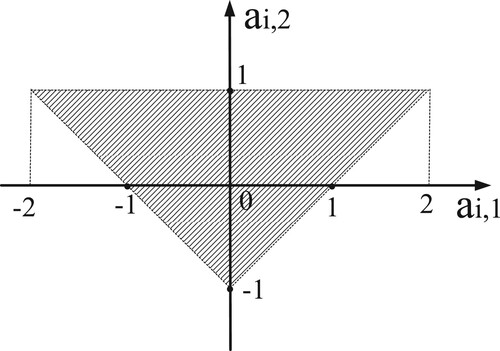In order to make sure that each $C_i\left(z\right)$ is stable, $C_i\left(z\right)$'s denominator-coefficients $a_{i,1}$ and $a_{i,2}$ must meet (3) $\begin{array}{cc}& \left|a_{i,2}\right|<1\\ & \left|a_{i,1}\right|<1+a_{i,2}.\end{array}$(3) The stability condition in (3(3) $\begin{array}{cc}& \left|a_{i,2}\right|<1\\ & \left|a_{i,1}\right|<1+a_{i,2}.\end{array}$(3) ) defines a stable region, which is the shaded area inside the triangle depicted in Figure 1. The triangle illustrated in Figure 1 is well known as stability triangle, and the stability requirement in (3(3) $\begin{array}{cc}& \left|a_{i,2}\right|<1\\ & \left|a_{i,1}\right|<1+a_{i,2}.\end{array}$(3) ) indicates that the all the combinations $(a_{i,1},a_{i,2})$ must be positioned within the stability triangle. More specifically, the shaded area inside the triangle specifies the stable region, and all the combinations $(a_{i,1},a_{i,2})$ must be located in this shaded area. To ensure that the condition in (3(3) $\begin{array}{cc}& \left|a_{i,2}\right|<1\\ & \left|a_{i,1}\right|<1+a_{i,2}.\end{array}$(3) ) is met, one must force all the points $(a_{i,1},a_{i,2})$ to be positioned within this shaded area (Deng, 2014; Jackson, 1992). Moreover, it should be noted that the boundaries of the triangle do not belong to the stable region. That is, the dotted lines surrounding the shaded area belong to the unstable region, which do not meet the stability requirement.

Figure 1. Stability triangle.

Once the variable-bandwidth specification $C_{\mathrm{d}}(\omega ,\psi )$ is given, it is obvious that a specific value of the parameter ψ corresponds to a specific specification $C_{\mathrm{d}}(\omega ,\psi )$. As an example, we consider the problem of employing the above cascade-form $C\left(z\right)$ to approximate a specific specification $C_{\mathrm{d}}(\omega ,\psi )$. To accomplish this objective, the filter coefficients $\left[\begin{array}{ccccc}g& b_{i,1}& b_{i,2}& a_{i,1}& a_{i,2}\end{array}\right]$must be optimized to best fit the specific $C_{\mathrm{d}}(\omega ,\psi )$. In this case, if the denominator-coefficients $(a_{i,1},a_{i,2})$ are directly optimized, $(a_{i,1},a_{i,2})$ may escape the shaded area (stable region) in Figure 1 and thus violate the condition in (3(3) $\begin{array}{cc}& \left|a_{i,2}\right|<1\\ & \left|a_{i,1}\right|<1+a_{i,2}.\end{array}$(3) ). This incurs instability, and thus makes the resulting filter $C\left(z\right)$ useless.

To constrain the locations of $(a_{i,1},a_{i,2})$ within the stability triangle, this paper adopts the technique employing coefficient transformations (4) $\{\begin{array}{l}{a}_{i,2}=\lambda \cdot \sin x_{i,2}\\ a_{i,1}=\lambda \cdot \sin x_{i,1}(1+a_{i,2}).\end{array}$(4) In the above transformations, the constant λ is constrained to be $0<\lambda <1$. Without this scaling parameter, the above transformations may fail to meet the stability requirement in (3(3) $\begin{array}{cc}& \left|a_{i,2}\right|<1\\ & \left|a_{i,1}\right|<1+a_{i,2}.\end{array}$(3) ). In Deng (1997), the constant λ is not included, which is under the assumptions that the unknowns $x_{i,2}$ and $x_{i,1}$ will never take the values (5) $\begin{array}{cc}{x}_{i,2}& =\pi /2+\mathrm{p\pi }\\ x_{i,1}& =\pi /2+\mathrm{q\pi }\end{array}$(5) and $p,q$ are any integers. Therefore, the transformations in (4(4) $\{\begin{array}{l}{a}_{i,2}=\lambda \cdot \sin x_{i,2}\\ a_{i,1}=\lambda \cdot \sin x_{i,1}(1+a_{i,2}).\end{array}$(4) ) remove such assumptions and thus theoretically guarantee that the stability requirement in (3(3) $\begin{array}{cc}& \left|a_{i,2}\right|<1\\ & \left|a_{i,1}\right|<1+a_{i,2}.\end{array}$(3) ) is absolutely satisfied. This means that the parameters $x_{i,1}$ and $x_{i,2}$ in (4(4) $\{\begin{array}{l}{a}_{i,2}=\lambda \cdot \sin x_{i,2}\\ a_{i,1}=\lambda \cdot \sin x_{i,1}(1+a_{i,2}).\end{array}$(4) ) are unconstrained, and no constraints like those in (5(5) $\begin{array}{cc}{x}_{i,2}& =\pi /2+\mathrm{p\pi }\\ x_{i,1}& =\pi /2+\mathrm{q\pi }\end{array}$(5) ) need to imposed on $x_{i,1}$ and $x_{i,2}$. Namely, arbitrary $x_{i,1}$ and $x_{i,2}$ absolutely satisfy the requirement in (3(3) $\begin{array}{cc}& \left|a_{i,2}\right|<1\\ & \left|a_{i,1}\right|<1+a_{i,2}.\end{array}$(3) ), which can be proved as follows. (6) $\begin{array}{rl}\left|a_{i,2}\right|& =|\lambda \cdot \sin x_{i,2}|\le \lambda <1\\ \left|a_{i,1}\right|& =|\lambda \cdot \sin x_{i,1}(1+a_{i,2}\left)\right|\\ & =|\lambda \cdot \sin x_{i,1}|(1+a_{i,2})\le \lambda (1+a_{i,2})<1+a_{i,2}.\end{array}$(6) Therefore, $x_{i,1}$ and $x_{i,2}$ become unconstrained parameters.

By inserting the coefficient transformations (4(4) $\{\begin{array}{l}{a}_{i,2}=\lambda \cdot \sin x_{i,2}\\ a_{i,1}=\lambda \cdot \sin x_{i,1}(1+a_{i,2}).\end{array}$(4) ) into $C_i\left(z\right)$ in (2(2) $C_i\left(z\right)=\frac{1+b_{i,1}{z}^{-1}+b_{i,2}{z}^{-2}}{1+a_{i,1}{z}^{-1}+a_{i,2}{z}^{-2}}$(2) ), the 2nd-order transfer function can be reshaped to (7) $C_i\left(z\right)=\frac{1+b_{i,1}{z}^{-1}+b_{i,2}{z}^{-2}}{1+\lambda \cdot \sin x_{i,1}(1+\lambda \cdot \sin x_{i,2})z^{-1}+\lambda \cdot \sin x_{i,2}{z}^{-2}}.$(7) After the above transformations are done, substituting $C_i\left(z\right)$ in (7(7) $C_i\left(z\right)=\frac{1+b_{i,1}{z}^{-1}+b_{i,2}{z}^{-2}}{1+\lambda \cdot \sin x_{i,1}(1+\lambda \cdot \sin x_{i,2})z^{-1}+\lambda \cdot \sin x_{i,2}{z}^{-2}}.$(7) ) into (1(1) $C\left(z\right)=g\cdot \prod _{i=1}^I{C}_i\left(z\right)$(1) ) yields the cascade-form recursive filter (constant filter) (8) $C\left(z\right)=g\cdot \prod _{i=1}^I\frac{1+b_{i,1}{z}^{-1}+b_{i,2}{z}^{-2}}{1+\lambda \cdot \sin x_{i,1}(1+\lambda \cdot \sin x_{i,2})z^{-1}+\lambda \cdot \sin x_{i,2}{z}^{-2}}.$(8) It is clear from (8(8) $C\left(z\right)=g\cdot \prod _{i=1}^I\frac{1+b_{i,1}{z}^{-1}+b_{i,2}{z}^{-2}}{1+\lambda \cdot \sin x_{i,1}(1+\lambda \cdot \sin x_{i,2})z^{-1}+\lambda \cdot \sin x_{i,2}{z}^{-2}}.$(8) ) that the unknowns to be optimized are (9) $\left[\begin{array}{ccccc}g& b_{i,1}& b_{i,2}& x_{i,1}& x_{i,2}\end{array}\right]$(9) for $i=1,2,\dots ,I$. Those unknowns can be optimized by using a nonlinear optimizer such that a specific cost function is minimized. Without any constraints on the new unknowns $x_{i,1}$ and $x_{i,2}$, the resulting 2nd-order transfer functions $C_i\left(z\right)$ is ensured to be stable. Since all the sections $C_i\left(z\right)$ are stable, the cascade-form $C\left(z\right)$ is also stable.

In the following subsection, this coefficient-transformation tactic is generalized to the case of designing a cascade-form variable-bandwidth recursive filter. The generalization to the variable-bandwidth case is of paramount importance because a variable-bandwidth filter updates its coefficients frequently, and may cause instability. In other words, since the coefficients of a variable-bandwidth filter are no longer fixed, changing the coefficients may incur instability. For this reason, ensuring the stability is of the paramount importance. In the design of a variable-bandwidth filter, the filter's coefficients are modelled as the functions of ψ. As ψ changes its values, $(a_{i,1},a_{i,2})$ may incur the violation of the stability condition and thus risk the instability. For this reason, it is vital that the stability is ensured for every single change of the value of ψ.

2.2. Two-step design procedure

Once the variable-bandwidth specification $C_{\mathrm{d}}(\omega ,\psi )$ is specified, it is approximated by employing the cascade-form transfer function (10) $C(z,\psi )=g\left(\psi \right)\cdot \prod _{i=1}^I{C}_i(z,\psi )$(10) where $g\left(\psi \right)$ represents the polynomial in ψ, and (11) $C_i(z,\psi )=\frac{1+b_{i,1}\left(\psi \right)z^{-1}+b_{i,2}\left(\psi \right)z^{-2}}{1+a_{i,1}\left(\psi \right)z^{-1}+a_{i,2}\left(\psi \right)z^{-2}}$(11) are the 2nd-order transfer functions (sections). In (11(11) $C_i(z,\psi )=\frac{1+b_{i,1}\left(\psi \right)z^{-1}+b_{i,2}\left(\psi \right)z^{-2}}{1+a_{i,1}\left(\psi \right)z^{-1}+a_{i,2}\left(\psi \right)z^{-2}}$(11) ), the numerator-coefficients $b_{i,1}\left(\psi \right)$ and $b_{i,2}\left(\psi \right)$ are the polynomials in ψ, while $a_{i,1}\left(\psi \right),a_{i,2}\left(\psi \right)$ can be attained by employing the transformations (12) $\{\begin{array}{l}{a}_{i,2}\left(\psi \right)=\lambda \cdot \sin x_{i,2}\left(\psi \right)\\ a_{i,1}\left(\psi \right)=\lambda \cdot \sin x_{i,1}\left(\psi \right)(1+a_{i,2}(\psi \left)\right).\end{array}$(12) Here, $x_{i,1}\left(\psi \right)$ and $x_{i,2}\left(\psi \right)$ also represent polynomials in ψ, but they are transformed to $a_{i,1}\left(\psi \right)$ and $a_{i,2}\left(\psi \right)$ as (12(12) $\{\begin{array}{l}{a}_{i,2}\left(\psi \right)=\lambda \cdot \sin x_{i,2}\left(\psi \right)\\ a_{i,1}\left(\psi \right)=\lambda \cdot \sin x_{i,1}\left(\psi \right)(1+a_{i,2}(\psi \left)\right).\end{array}$(12) ) for the stability reason. As can be seen from (10(10) $C(z,\psi )=g\left(\psi \right)\cdot \prod _{i=1}^I{C}_i(z,\psi )$(10) ), $g\left(\psi \right)$ is used to scale the cascade of the 2nd-order transfer functions.

As proved in (6(6) $\begin{array}{rl}\left|a_{i,2}\right|& =|\lambda \cdot \sin x_{i,2}|\le \lambda <1\\ \left|a_{i,1}\right|& =|\lambda \cdot \sin x_{i,1}(1+a_{i,2}\left)\right|\\ & =|\lambda \cdot \sin x_{i,1}|(1+a_{i,2})\le \lambda (1+a_{i,2})<1+a_{i,2}.\end{array}$(6) ), even if $x_{i,1}\left(\psi \right)$ and $x_{i,2}\left(\psi \right)$ are arbitrary polynomials, they will not violate the stability condition. That is, arbitrary polynomials $x_{i,1}\left(\psi \right)$, $x_{i,2}\left(\psi \right)$ satisfy the stability requirement (13) $\{\begin{array}{l}\left|a_{i,2}\right(\psi \left)\right|<1\\ \left|a_{i,1}\right(\psi \left)\right|<1+a_{i,2}\left(\psi \right).\end{array}$(13) For clarifying the reason why no violation occurs, the detailed proof is given as follows. (14) $\begin{array}{rl}\left|a_{i,2}\right(\psi \left)\right|& =|\lambda \cdot \sin x_{i,2}(\psi \left)\right|\le \lambda <1\\ \left|a_{i,1}\right(\psi \left)\right|& =|\lambda \cdot \sin x_{i,1}(\psi \left)\right(1+a_{i,2}\left(\psi \right)\left)\right|\\ & =|\lambda \cdot \sin x_{i,1}(\psi \left)\right|(1+a_{i,2}(\psi \left)\right)\le \lambda (1+a_{i,2}(\psi \left)\right)<1+a_{i,2}\left(\psi \right).\end{array}$(14) As a consequence, one simply needs to determine the polynomials $\left[\begin{array}{ccccc}g\left(\psi \right)& b_{i,1}\left(\psi \right)& b_{i,2}\left(\psi \right)& x_{i,1}\left(\psi \right)& x_{i,2}\left(\psi \right)\end{array}\right]$in approximating the given variable-bandwidth magnitude-specification $C_{\mathrm{d}}(\omega ,\psi )$. In this paper, the least-squares error criterion is employed, and the following 2-step procedure is applied.

Step-1:

$\psi \in [{\psi }_{min},{\psi }_{max}]$ is evenly discretized to get L evenly-spaced samples $\psi \left(l\right)$. Those samples lead to the discretized specifications $C_{\mathrm{d}}(\omega ,\psi (l\left)\right).$ After getting the samples $C_{\mathrm{d}}(\omega ,\psi (l\left)\right)$, each $C_{\mathrm{d}}(\omega ,\psi (l\left)\right)$ is approximated by using the transfer function $C\left(z\right)$ in (1(1) $C\left(z\right)=g\cdot \prod _{i=1}^I{C}_i\left(z\right)$(1) ). In such an approximation, we find the optimal factor g as well as the coefficients of each 2nd-order transfer function. Specifically, the coefficients contained in the vector (15) $\mathit{y}=\left[\begin{array}{ccccc}g& b_{i,1}& b_{i,2}& x_{i,1}& x_{i,2}\end{array}\right]$(15) are optimized, $i=1,2,\dots ,L$. This can be achieved by minimizing the squared error function (16) $f\left(\mathit{y}\right)=\sum _{\omega }{\left|\mathrm{\Delta }\right(\omega ,\psi \left(l\right)\left)\right|}^2$(16) where $\mathrm{\Delta }(\omega ,\psi (l\left)\right)=C_{\mathrm{d}}(\omega ,\psi (l\left)\right)-C\left(\omega \right)$represents the approximation error, $C\left(\omega \right)$ denotes the response of $C\left(z\right)$. When computing the magnitude response $C\left(\omega \right)$ from the cascaded transfer function in (8(8) $C\left(z\right)=g\cdot \prod _{i=1}^I\frac{1+b_{i,1}{z}^{-1}+b_{i,2}{z}^{-2}}{1+\lambda \cdot \sin x_{i,1}(1+\lambda \cdot \sin x_{i,2})z^{-1}+\lambda \cdot \sin x_{i,2}{z}^{-2}}.$(8) ), it is found that $C\left(\omega \right)$ is a highly nonlinear function of the unknowns in (15(15) $\mathit{y}=\left[\begin{array}{ccccc}g& b_{i,1}& b_{i,2}& x_{i,1}& x_{i,2}\end{array}\right]$(15) ). Therefore, minimizing the squared error $f\left(\mathit{y}\right)$ in (16(16) $f\left(\mathit{y}\right)=\sum _{\omega }{\left|\mathrm{\Delta }\right(\omega ,\psi \left(l\right)\left)\right|}^2$(16) ) is highly nonlinear. This highly nonlinear problem can only be solved by employing a nonlinear-programming tactic. In this study, the MATLAB function fminsearch (nonlinear minimizer) is used for minimizing the squared error $f\left(\mathit{y}\right)$. Evidently, after all the discretized specifications $C_{\mathrm{d}}(\omega ,\psi (l\left)\right)$ are approximated, this step yields L sets of the optimized unknowns (17) ${\mathit{y}}_l=\left[\begin{array}{ccccc}{g}^{\left(l\right)}& b_{i,1}^{\left(l\right)}& b_{i,2}^{\left(l\right)}& x_{i,1}^{\left(l\right)}& x_{i,2}^{\left(l\right)}\end{array}\right]$(17) $l=1,2,\dots ,L$. The L sets of the optimized values can be represented by using the matrix (18) $\mathit{Y}=\left[\begin{array}{ccccc}{g}^{\left(1\right)}& b_{i,1}^{\left(1\right)}& b_{i,2}^{\left(1\right)}& x_{i,1}^{\left(1\right)}& x_{i,2}^{\left(1\right)}\\ g^{\left(2\right)}& b_{i,1}^{\left(2\right)}& b_{i,2}^{\left(2\right)}& x_{i,1}^{\left(2\right)}& x_{i,2}^{\left(2\right)}\\ g^{\left(3\right)}& b_{i,1}^{\left(3\right)}& b_{i,2}^{\left(3\right)}& x_{i,1}^{\left(3\right)}& x_{i,2}^{\left(3\right)}\\ ⋮& ⋮& ⋮& ⋮& ⋮\\ g^{\left(L\right)}& b_{i,1}^{\left(L\right)}& b_{i,2}^{\left(L\right)}& x_{i,1}^{\left(L\right)}& x_{i,2}^{\left(L\right)}\end{array}\right]$(18) with each row representing the lth set of coefficients for approximating the lth specification $C_{\mathrm{d}}(\omega ,\psi (l\left)\right)$. In other words, each row lists the resulting coefficients of the lth constant-bandwidth recursive filter $C\left(z\right)$ in (1(1) $C\left(z\right)=g\cdot \prod _{i=1}^I{C}_i\left(z\right)$(1) ) for approximating the lth specification $C_{\mathrm{d}}(\omega ,\psi (l\left)\right)$. Since Step-1 produces L constant-bandwidth filters, the above matrix $\mathit{Y}$ contains L rows.

Step-2:

After the optimized coefficient values in (18(18) $\mathit{Y}=\left[\begin{array}{ccccc}{g}^{\left(1\right)}& b_{i,1}^{\left(1\right)}& b_{i,2}^{\left(1\right)}& x_{i,1}^{\left(1\right)}& x_{i,2}^{\left(1\right)}\\ g^{\left(2\right)}& b_{i,1}^{\left(2\right)}& b_{i,2}^{\left(2\right)}& x_{i,1}^{\left(2\right)}& x_{i,2}^{\left(2\right)}\\ g^{\left(3\right)}& b_{i,1}^{\left(3\right)}& b_{i,2}^{\left(3\right)}& x_{i,1}^{\left(3\right)}& x_{i,2}^{\left(3\right)}\\ ⋮& ⋮& ⋮& ⋮& ⋮\\ g^{\left(L\right)}& b_{i,1}^{\left(L\right)}& b_{i,2}^{\left(L\right)}& x_{i,1}^{\left(L\right)}& x_{i,2}^{\left(L\right)}\end{array}\right]$(18) ) are attained, each column is fitted by utilizing an individual polynomial in ψ. This curve-fitting results in the polynomials (19) $\left[\begin{array}{ccccc}g\left(\psi \right)& b_{i,1}\left(\psi \right)& b_{i,2}\left(\psi \right)& x_{i,1}\left(\psi \right)& x_{i,2}\left(\psi \right)\end{array}\right]$(19) for $i=1,2,\dots ,I$. Transforming $x_{i,1}\left(\psi \right)$ and $x_{i,2}\left(\psi \right)$ into (20) $\begin{array}{rl}{a}_{i,2}\left(\psi \right)& =\lambda \cdot \sin x_{i,2}\left(\psi \right)\\ a_{i,1}\left(\psi \right)& =\lambda \cdot \sin x_{i,1}\left(\psi \right)(1+a_{i,2}(\psi \left)\right)\end{array}$(20) attains the coefficients $a_{i,1}\left(\psi \right)$ and $a_{i,2}\left(\psi \right)$ that are the denominator coefficients of the 2nd-order transfer functions given in (11(11) $C_i(z,\psi )=\frac{1+b_{i,1}\left(\psi \right)z^{-1}+b_{i,2}\left(\psi \right)z^{-2}}{1+a_{i,1}\left(\psi \right)z^{-1}+a_{i,2}\left(\psi \right)z^{-2}}$(11) ). As a consequence, the variable-bandwidth filter $C(z,\psi )$ in (10(10) $C(z,\psi )=g\left(\psi \right)\cdot \prod _{i=1}^I{C}_i(z,\psi )$(10) ) has the coefficients (21) $\left[\begin{array}{ccccc}g\left(\psi \right)& b_{i,1}\left(\psi \right)& b_{i,2}\left(\psi \right)& a_{i,1}\left(\psi \right)& a_{i,2}\left(\psi \right)\end{array}\right].$(21)

It should be noted again that $g\left(\psi \right),b_{i,1}\left(\psi \right),b_{i,2}\left(\psi \right)$ are the direct results from the above polynomial fitting, while $a_{i,1}\left(\psi \right)$ and $a_{i,2}\left(\psi \right)$ must be obtained using the transformations in (20(20) $\begin{array}{rl}{a}_{i,2}\left(\psi \right)& =\lambda \cdot \sin x_{i,2}\left(\psi \right)\\ a_{i,1}\left(\psi \right)& =\lambda \cdot \sin x_{i,1}\left(\psi \right)(1+a_{i,2}(\psi \left)\right)\end{array}$(20) ) for the stability purpose. Once those coefficients (functions) are available, changing the value of ψ in (21(21) $\left[\begin{array}{ccccc}g\left(\psi \right)& b_{i,1}\left(\psi \right)& b_{i,2}\left(\psi \right)& a_{i,1}\left(\psi \right)& a_{i,2}\left(\psi \right)\end{array}\right].$(21) ) updates the coefficient values of the variable-bandwidth filter $C(z,\psi )$, and thus yields an updated bandwidth response. Thus, the variable-bandwidth recursive filter can be attained by following the above two steps (Step-1 and Step-2).

As will be shown in the following section, the stability of the designed $C(z,\psi )$ can be verified by employing the stability triangles, while the approximation performance can be assessed by using the following two error criteria. One is the normalized RMS error (22) ${\delta }_{\mathrm{rms}}=\sqrt{\frac{{\displaystyle \sum _{\omega ,\psi }\left|\mathrm{\Delta }\right(\omega ,\psi ){|}^2}}{{\displaystyle \sum _{\omega ,\psi }\left|C_{\mathrm{d}}\right(\omega ,\psi ){|}^2}}}\times 100\text{\%}$(22) and another error criterion is the maximum error (23) ${\delta }_{max}=max\left\{\right|\mathrm{\Delta }(\omega ,\psi )\left|\right\}$(23) where (24) $\mathrm{\Delta }(\omega ,\psi )=C_{\mathrm{d}}(\omega ,\psi )-C(\omega ,\psi )$(24) denotes the approximation error, $C(\omega ,\psi )$ denotes the variable-bandwidth response of the designed filter $C(z,\psi )$, and ω and ψ denote evenly-spaced samples used for assessing the approximation performance.

3. Computer simulation results

This section gives an example that shows how to design a cascade-form lowpass variable-bandwidth filter by employing the 2-step procedure. The lowpass filter has tuneable passband-width and tuneable stopband-width, but its transition-bandwidth remains unchanged. Simulation results are included for verifying the attained stability as well as demonstrating the high approximation accuracy.

The variable-bandwidth specification $C_{\mathrm{d}}(\omega ,\psi )$ is specified by (25) $C_{\mathrm{d}}(\omega ,\psi )=\{\begin{array}{cc}1& 0\le |\omega |\le {\omega }_{\mathrm{p}}\\ \frac{{\omega }_{\mathrm{s}}-\omega }{{\omega }_{\mathrm{s}}-{\omega }_{\mathrm{p}}}& {\omega }_{\mathrm{p}}\le |\omega |\le {\omega }_{\mathrm{s}}\\ 0& {\omega }_{\mathrm{s}}\le |\omega |\le \pi \end{array}$(25) with (26) $\begin{array}{cc}& {\omega }_{\mathrm{p}}=0.26\pi +\psi \\ & {\omega }_{\mathrm{s}}=0.50\pi +\psi \\ & \psi \in [-0.16\pi ,0.16\pi ].\end{array}$(26) In (25(25) $C_{\mathrm{d}}(\omega ,\psi )=\{\begin{array}{cc}1& 0\le |\omega |\le {\omega }_{\mathrm{p}}\\ \frac{{\omega }_{\mathrm{s}}-\omega }{{\omega }_{\mathrm{s}}-{\omega }_{\mathrm{p}}}& {\omega }_{\mathrm{p}}\le |\omega |\le {\omega }_{\mathrm{s}}\\ 0& {\omega }_{\mathrm{s}}\le |\omega |\le \pi \end{array}$(25) ), ${\omega }_{\mathrm{p}}$ denotes the edge-frequency of the passband $\omega \in [0,{\omega }_{\mathrm{p}}]$, and ${\omega }_{\mathrm{s}}$ denotes the edge-frequency of the stopband $\omega \in [{\omega }_{\mathrm{s}},\pi ]$. Furthermore, the parameter ψ is adopted for tuning both ${\omega }_{\mathrm{p}}$ and ${\omega }_{\mathrm{s}}$. As ψ varies within $[-0.16\pi ,0.16\pi ]$, both passband-width and stopband-width can be updated continuously. In addition, the transition-bandwidth keeps constant, which equals $0.24\pi$.

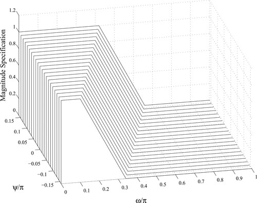
To begin the 2-step design, both frequency ω and parameter ψ must be discretized. In the computer simulations, 21 evenly-spaced samples of ψ are taken from $\psi \in [-0.16\pi ,0.16\pi ]$, i.e. $L=21$, and 1001 evenly-spaced samples of ω are taken from $\omega \in [0,\pi ]$. The discretized variable-bandwidth specifications $C_{\mathrm{d}}(\omega ,\psi )$ are plotted in Figure 2, where $L=21$ curves represent the discretized $C_{\mathrm{d}}(\omega ,\psi )$. Equivalently, those curves are the individual specifications $C_{\mathrm{d}}(\omega ,\psi (l\left)\right)$ that are to be approximated in Step-1.

Figure 2. Discretized specifications $C_{\mathrm{d}}(\omega ,\psi (l\left)\right)$, $l=1,2,\dots ,L$.

Here, we employ the 2-step procedure detailed in the preceding section to get a stable variable-bandwidth recursive filter. Step-1 designs L constant-bandwidth recursive lowpass filters for approximating the discretized L lowpass specifications $C_{\mathrm{d}}(\omega ,\psi (l\left)\right)$ given in Figure 2. Those constant-bandwidth lowpass filters are separately designed, and the filter order is 4, which corresponds to I = 2 in (1(1) $C\left(z\right)=g\cdot \prod _{i=1}^I{C}_i\left(z\right)$(1) ). This means that two 2nd-order recursive transfer functions are cascaded to construct the fourth-order (I = 2) constant-bandwidth filter. Step-1 begins designing the first constant-bandwidth lowpass filter that approximates the first lowpass specification $C_{\mathrm{d}}(\omega ,\psi (1\left)\right)$. This approximation needs a nonlinear minimizer to minimize the squared error in (16(16) $f\left(\mathit{y}\right)=\sum _{\omega }{\left|\mathrm{\Delta }\right(\omega ,\psi \left(l\right)\left)\right|}^2$(16) ). This study employs the MATLAB function fminsearch in the nonlinear minimization. Moreover, the nonlinear minimization requires a set of initial values of the unknowns to start. Here, all the initial values are chosen to be zero, i.e. (27) $\left[\begin{array}{c}g\\ b_{1,1}\\ b_{1,2}\\ b_{2,1}\\ b_{2,2}\\ x_{1,2}\\ x_{1,1}\\ x_{2,2}\\ x_{2,1}\end{array}\right]=\left[\begin{array}{c}0\\ 0\\ 0\\ 0\\ 0\\ 0\\ 0\\ 0\\ 0\end{array}\right].$(27) Furthermore, the parameter λ used for the coefficient-transformations in (4(4) $\{\begin{array}{l}{a}_{i,2}=\lambda \cdot \sin x_{i,2}\\ a_{i,1}=\lambda \cdot \sin x_{i,1}(1+a_{i,2}).\end{array}$(4) ) is $\lambda =1-ϵ,ϵ={10}^{-5}.$The nonlinear minimization involves a repeated iteration, and it must be terminated once a stopping criterion is met. Here, the iteration is stopped once the difference of two succeeding normalized RMS errors ${\delta }_{\mathrm{rms}}$ as defined in (22(22) ${\delta }_{\mathrm{rms}}=\sqrt{\frac{{\displaystyle \sum _{\omega ,\psi }\left|\mathrm{\Delta }\right(\omega ,\psi ){|}^2}}{{\displaystyle \sum _{\omega ,\psi }\left|C_{\mathrm{d}}\right(\omega ,\psi ){|}^2}}}\times 100\text{\%}$(22) ) is less than a preset threshold, say, $\eta ={10}^{-5}\text{\%}$. After the design of the first constant-bandwidth recursive filter is completed, the optimized values of the unknowns in (27(27) $\left[\begin{array}{c}g\\ b_{1,1}\\ b_{1,2}\\ b_{2,1}\\ b_{2,2}\\ x_{1,2}\\ x_{1,1}\\ x_{2,2}\\ x_{2,1}\end{array}\right]=\left[\begin{array}{c}0\\ 0\\ 0\\ 0\\ 0\\ 0\\ 0\\ 0\\ 0\end{array}\right].$(27) ) are exploited as the initial point for starting the design of the next constant-bandwidth lowpass filter, aiming to approximate the second lowpass specification $C_{\mathrm{d}}(\omega ,\psi (2\left)\right)$. This procedure is iterated until the design of the last (Lth) constant-bandwidth lowpass filter is completed, i.e. approximating the last specification $C_{\mathrm{d}}(\omega ,\psi (L\left)\right)$ is done. Figure 3 plots the resultant lowpass responses of the obtained constant-bandwidth lowpass filters ($L=21$). Based on the error criteria defined in (22(22) ${\delta }_{\mathrm{rms}}=\sqrt{\frac{{\displaystyle \sum _{\omega ,\psi }\left|\mathrm{\Delta }\right(\omega ,\psi ){|}^2}}{{\displaystyle \sum _{\omega ,\psi }\left|C_{\mathrm{d}}\right(\omega ,\psi ){|}^2}}}\times 100\text{\%}$(22) ) and (23(23) ${\delta }_{max}=max\left\{\right|\mathrm{\Delta }(\omega ,\psi )\left|\right\}$(23) ), the average of the L = 21 normalized RMS errors ${\delta }_{\mathrm{rms}}$ is ${\overline{\delta }}_{\mathrm{rms}}=2.6468\text{\%},$while the average of the $L=21$ maximum errors ${\delta }_{max}$ is ${\overline{\delta }}_{max}=\mathrm{0.0552.}$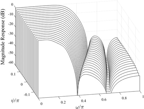In addition, Figure 4 gives the resultant lowpass responses in decibel (dB) of the designed L constant-bandwidth lowpass filters. Once designing the constant-bandwidth filters ($L=21$) is completed, all the optimized values of the unknowns in (27(27) $\left[\begin{array}{c}g\\ b_{1,1}\\ b_{1,2}\\ b_{2,1}\\ b_{2,2}\\ x_{1,2}\\ x_{1,1}\\ x_{2,2}\\ x_{2,1}\end{array}\right]=\left[\begin{array}{c}0\\ 0\\ 0\\ 0\\ 0\\ 0\\ 0\\ 0\\ 0\end{array}\right].$(27) ) are available. Then, those optimized values are individually fitted by using distinct polynomials. For example, the polynomial $g\left(\psi \right)$ is employed to fit all the optimized values of g by minimizing the squared fitting error. Repeating the same fitting procedure produces the 9 polynomials (28) $\left[\begin{array}{c}g\left(\psi \right)\\ b_{1,1}\left(\psi \right)\\ b_{1,2}\left(\psi \right)\\ b_{2,1}\left(\psi \right)\\ b_{2,2}\left(\psi \right)\\ x_{1,2}\left(\psi \right)\\ x_{1,1}\left(\psi \right)\\ x_{2,2}\left(\psi \right)\\ x_{2,1}\left(\psi \right)\end{array}\right].$(28) The problem here is how to decide the polynomial degrees. Computer simulations have found that those polynomials do not necessarily need the same degree. For some of the polynomials in (28(28) $\left[\begin{array}{c}g\left(\psi \right)\\ b_{1,1}\left(\psi \right)\\ b_{1,2}\left(\psi \right)\\ b_{2,1}\left(\psi \right)\\ b_{2,2}\left(\psi \right)\\ x_{1,2}\left(\psi \right)\\ x_{1,1}\left(\psi \right)\\ x_{2,2}\left(\psi \right)\\ x_{2,1}\left(\psi \right)\end{array}\right].$(28) ), relatively low degrees suffice, while for some others, low degrees tend to cause an increased design error. For this reason, the criterion used here for choosing the polynomial degrees is to see if or not the increase of the normalized RMS error ${\delta }_{\mathrm{rms}}$ exceeds a predetermined threshold. Here, the trial-and-error policy is adopted. Specifically, all the polynomial degrees are first set the same, for example, the third-degree is first set for all the polynomials in (28(28) $\left[\begin{array}{c}g\left(\psi \right)\\ b_{1,1}\left(\psi \right)\\ b_{1,2}\left(\psi \right)\\ b_{2,1}\left(\psi \right)\\ b_{2,2}\left(\psi \right)\\ x_{1,2}\left(\psi \right)\\ x_{1,1}\left(\psi \right)\\ x_{2,2}\left(\psi \right)\\ x_{2,1}\left(\psi \right)\end{array}\right].$(28) ). Then, the degree of only one of the polynomials is reduced by one, and the increase of the error ${\delta }_{\mathrm{rms}}$ is investigated. If the increase of ${\delta }_{\mathrm{rms}}$ is less than $0.1\text{\%}$, that degree can be reduced by one. Otherwise, the degree cannot be reduced, and that degree is kept unchanged. In this way, such trial-and-error executions result in the polynomial degrees (29) $\left[\begin{array}{ccccccccc}g\left(\psi \right)& b_{1,1}\left(\psi \right)& b_{1,2}\left(\psi \right)& b_{2,1}\left(\psi \right)& b_{2,2}\left(\psi \right)& x_{1,2}\left(\psi \right)& x_{1,1}\left(\psi \right)& x_{2,2}\left(\psi \right)& x_{2,1}\left(\psi \right)\\ \updownarrow & \updownarrow & \updownarrow & \updownarrow & \updownarrow & \updownarrow & \updownarrow & \updownarrow & \updownarrow \\ 3& 2& 1& 3& 1& 2& 2& 2& 2\end{array}\right].$(29) By employing the obtained polynomial degrees in (29(29) $\left[\begin{array}{ccccccccc}g\left(\psi \right)& b_{1,1}\left(\psi \right)& b_{1,2}\left(\psi \right)& b_{2,1}\left(\psi \right)& b_{2,2}\left(\psi \right)& x_{1,2}\left(\psi \right)& x_{1,1}\left(\psi \right)& x_{2,2}\left(\psi \right)& x_{2,1}\left(\psi \right)\\ \updownarrow & \updownarrow & \updownarrow & \updownarrow & \updownarrow & \updownarrow & \updownarrow & \updownarrow & \updownarrow \\ 3& 2& 1& 3& 1& 2& 2& 2& 2\end{array}\right].$(29) ), one can get all the polynomials in (28(28) $\left[\begin{array}{c}g\left(\psi \right)\\ b_{1,1}\left(\psi \right)\\ b_{1,2}\left(\psi \right)\\ b_{2,1}\left(\psi \right)\\ b_{2,2}\left(\psi \right)\\ x_{1,2}\left(\psi \right)\\ x_{1,1}\left(\psi \right)\\ x_{2,2}\left(\psi \right)\\ x_{2,1}\left(\psi \right)\end{array}\right].$(28) ).

Figure 3. Constant-bandwidth lowpass responses from Step-1.

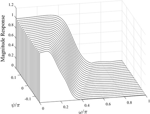
Figure 4. Constant-bandwidth lowpass responses (dB) from Step-1.

Figure 5 depicts all the 9 fitted polynomials listed in (28(28) $\left[\begin{array}{c}g\left(\psi \right)\\ b_{1,1}\left(\psi \right)\\ b_{1,2}\left(\psi \right)\\ b_{2,1}\left(\psi \right)\\ b_{2,2}\left(\psi \right)\\ x_{1,2}\left(\psi \right)\\ x_{1,1}\left(\psi \right)\\ x_{2,2}\left(\psi \right)\\ x_{2,1}\left(\psi \right)\end{array}\right].$(28) ). In Figure 5, the circles show the optimized values of the unknowns in (27(27) $\left[\begin{array}{c}g\\ b_{1,1}\\ b_{1,2}\\ b_{2,1}\\ b_{2,2}\\ x_{1,2}\\ x_{1,1}\\ x_{2,2}\\ x_{2,1}\end{array}\right]=\left[\begin{array}{c}0\\ 0\\ 0\\ 0\\ 0\\ 0\\ 0\\ 0\\ 0\end{array}\right].$(27) ), which are the results of the designed constant-bandwidth lowpass filters from Step-1, while the solid lines show the 9 polynomials fitted in Step-2. Figure 6 plots the lowpass responses of the obtained lowpass variable-bandwidth filter, where more evenly-spaced samples ($L=41$) of ψ are taken from $[-0.16\pi ,0.16\pi ]$. This is because using denser samples enables the designer to scrutinize the approximation accuracy in-between the samples that are utilized in the designs of the constant-bandwidth filters (Step-1). It is clear from Figure 6 that both the passband-width and stopband-width vary continuously. Computing the average of the $L=41$ normalized RMS errors ${\delta }_{\mathrm{rms}}$ yields ${\overline{\delta }}_{\mathrm{rms}}=2.9562\text{\%},$while the average of the $L=41$ maximum deviations ${\delta }_{max}$ is ${\overline{\delta }}_{max}=\mathrm{0.0555.}$One can conclude that the approximation accuracy is considerably high. 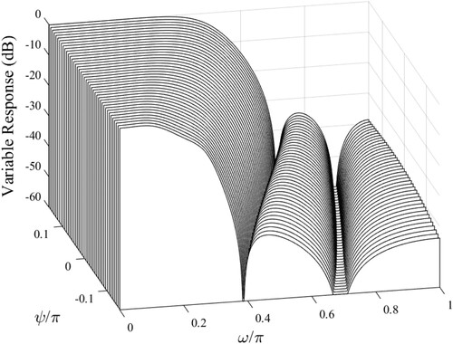This is because the differences between the average errors (both the normalized RMS error ${\delta }_{\mathrm{rms}}$ and the maximum error ${\delta }_{max}$) of the constant-bandwidth filters (Step-1) and the final variable-bandwidth filter (Step-2) are negligibly small. Furthermore, Figure 7 plots the variable-bandwidth lowpass responses in decibel (dB) of the attained variable lowpass filter.

Figure 5. Polynomials obtained from Step-2 (9 polynomials).

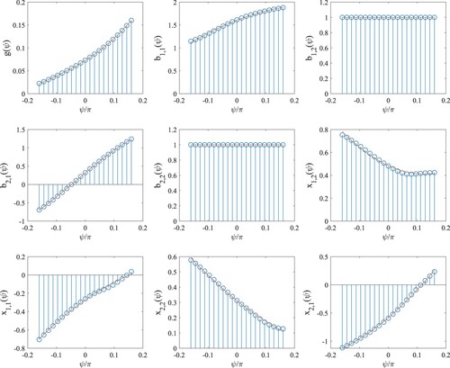
Figure 6. Variable-bandwidth lowpass responses from Step-2.

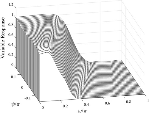
Figure 7. Variable-bandwidth lowpass responses (dB) from Step-2.

To prove that the obtained constant-bandwidth filters satisfy the stability requirement, Figure 8 illustrates the configurations of $(a_{1,1},a_{1,2})$ and $(a_{2,1},a_{2,2})$. It is seen from Figure 8 that all the combinations $(a_{1,1},a_{1,2})$ and $(a_{2,1},a_{2,2})$ always stay inside the triangles. Therefore, all the resultant constant-bandwidth filters remain stable even if ψ changes its values.

Figure 8. Stability triangles from Step-1 (constant-bandwidth filters).

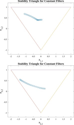
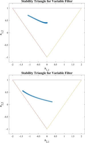
Next, let us investigate the stability of the resulting cascade-form variable-bandwidth lowpass filter $C(z,\psi )$. Figure 9 shows the first combination pair $\left(a_{1,1}\right(\psi ),a_{1,2}(\psi \left)\right)$ as well as the second combination pair $\left(a_{2,1}\right(\psi ),a_{2,2}(\psi \left)\right)$. As can be observed from Figure 9, as the parameter ψ changes its values, both $\left(a_{1,1}\right(\psi ),a_{1,2}(\psi \left)\right)$ and $\left(a_{2,1}\right(\psi ),a_{2,2}(\psi \left)\right)$ always stay inside the triangles. This concludes that the obtained variable-bandwidth recursive lowpass filter $C(z,\psi )$ always remains stable despite the change of the ψ values within the range $[-0.16\pi ,0.16\pi ]$.

Figure 9. Stability triangles from Step-2 (variable-bandwidth filter).

Finally, let us compare the simulation results here with those in Deng (1997). In Deng (1997), the average of the normalized RMS error ${\delta }_{\mathrm{rms}}$ is ${\overline{\delta }}_{\mathrm{rms}}=3.4544\text{\%},$while the average of the maximum deviations ${\delta }_{max}$ is ${\overline{\delta }}_{max}=\mathrm{0.0614.}$Moreover, the fourth-degree polynomials are employed in Deng (1997), whereas this paper uses lower-degree polynomials. Even if lower-degree polynomials are employed in this paper, the approximation accuracy is higher. It should be pointed out that utilizing lower-degree polynomials reduces the complexity needed in implementing the designed variable-bandwidth lowpass filter. As a conclusion, the 2-step design employing the cascade-form structure not only leads to the hardware implementation with low round-off noises, but also can achieve higher approximation accuracy. Moreover, the stability of the attained variable-bandwidth lowpass filter is absolutely ensured.

4. Conclusions

In this paper, the cascade-form structure has been introduced for designing a variable-bandwidth recursive filter using a 2-step procedure. The cascade-form structure consists of cascaded 2nd-order transfer functions, and it features low coefficient-sensitivity in terms of low round-off noises when it is implemented using hardwares. The 2-step procedure first uses a nonlinear minimization algorithm to design a series of constant-bandwidth recursive filters (Step-1), and then fits the optimized values of each unknown by using an individual polynomial (Step-2). To ensure the stability of the cascade-form filters (both constant-bandwidth and variable-bandwidth filters), coefficient transformations are adopted, aiming to force the coefficients in the denominator of each 2nd-order section to be located inside the shaded area (stable region) shown in Figure 1. A lowpass example is included to show that the resulting variable-bandwidth recursive filter exhibits the following advantages.

• The stability is definitely guaranteed, which comes from the coefficient transformations;

• The approximation accuracy is higher even if the degree of the fitting polynomials is lower as compared with the existing results in Deng (1997);

• The cascade-form structure facilitates the hardware implementations, where the 2nd-order transfer functions can be taken as the basic building modules;

• The cascade-form structure features low round-off noises for hardware implementations as compared with the existing direct-form structures.

Disclosure statement

No potential conflict of interest was reported by the author(s).

References

- Deng, T.-B. (1997). Design of recursive 1-D variable filters with guaranteed stability. IEEE Transactions on Circuits and Systems II: Analog Digital Signal Processing, 44(9), 689–695.
- Deng, T.-B. (1998). New method for designing stable recursive variable digital filters. Signal Processing, 64(2), 197–207. https://doi.org/10.1016/S0165-1684(97)00188-6
- Deng, T.-B. (2001a). An improved method for designing variable recursive digital filters with guaranteed stability. Signal Processing, 81(2), 439–446. https://doi.org/10.1016/S0165-1684(00)00220-6
- Deng, T.-B. (2001b). Discretization-free design of variable fractional-delay FIR digital filters. IEEE Transactions on Circuits and Systems II, Analog Digital Signal Processing, 48(6), 637–644. https://doi.org/10.1109/82.943337
- Deng, T.-B. (2004). Closed-form design and efficient implementation of variable digital filters with simultaneously tuneable magnitude and fractional-delay. IEEE Transactions on Signal Processing, 52(6), 1668–1681. https://doi.org/10.1109/TSP.2004.827150
- Deng, T.-B. (2014, Oct. 22–25). Variable-recursive-filter design with theoretical stability-guarantee. In Proc. IEEE TENCON 2014 (pp. 1–5). Bangkok, Thailand.
- Deng, T.-B. (2016). Design of recursive variable-digital-filters with theoretically-guaranteed stability. International Journal of Electronics, 103(12), 2013–2028. https://doi.org/10.1080/00207217.2016.1175033
- Deng, T.-B. (2018). The Lp-norm-minimization design of stable variable-bandwidth digital filters. Journal of Circuits, Systems, and Computers, 27(7), Article 1850102, 1–18. https://doi.org/10.1142/S0218126618501025
- Deng, T.-B. (2023). Various unity-bounded functions for designing recursive digital filters with variable notch-frequency and guaranteed stability. Journal of Circuits, Systems, and Computers, 32(6), Article 2350095, 1–22. https://doi.org/10.1142/S0218126623500950
- Deng, T.-B., & Lian, Y. (2006). Weighted-least-squares design of variable fractional-delay FIR filters using coefficient-symmetry. IEEE Transactions on Signal Processing, 54(8), 3023–3038. https://doi.org/10.1109/TSP.2006.875385
- Deng, T.-B., & Nakagawa, Y. (2004). SVD-based design and new structures for variable fractional-delay digital filters. IEEE Transactions on Signal Processing, 52(9), 2513–2527. https://doi.org/10.1109/TSP.2004.831922
- Farrow, C. W. (1988). A continuously variable digital delay element. In Proc. 1988 IEEE Int. Symp. Circuits Syst. (pp. 2641–2645).
- Jackson, L. B. (1992). Digital filters and signa processing (2nd ed.). Kluwer Academic Publishers.
- Shyu, J.-J., Pei, S.-C., & Huang, Y.-D. (2009). Design of variable two-dimensional FIR digital filters by McClellan transformation. IEEE Transactions on Circuits and Systems I: Regular Papers, 56(3), 574–582. https://doi.org/10.1109/TCSI.2008.2002119
- Soontornwong, P., Deng, T.-B., & Chivapreecha, S. (2017). Low-complexity and high-modularity structure for implementing transient-free Pascal-delay filter. IEEE Transactions on Signal Processing, 65(23), 6233–6243. https://doi.org/10.1109/TSP.2017.2750117
- Sutthikarn, P., Chivapreecha, S., Trirat, A., & Jongsataporn, T. (2020). A simple tunable biquadratic digital bandpass filter design for spectrum sensing in cognitive radio. In Proc. IEEE ECTI-CON 2020 (pp. 71–75).
- Zarour, R., & Fahmy, M. M. (1989a). A design technique for variable digital filters. IEEE Transactions on Circuits and Systems, 36(11), 1473–1478. https://doi.org/10.1109/31.41307
- Zarour, R., & Fahmy, M. M. (1989b). A design technique for variable two-dimensional recursive digital filters. Signal Processing, 17(2), 175–182. https://doi.org/10.1016/0165-1684(89)90021-2