On finite mixture models

ABSTRACT

Finite mixture models are widely used in scientific investigations. Due to their non-regularity, there are many technical challenges concerning inference problems on various aspects of the finite mixture models. After decades of effort by statisticians, substantial progresses are recorded recently in characterising large sample properties of some classical inference methods when applied to finite mixture models, providing effective numerical solutions for mixture model-based data analysis, and the invention of novel inference approaches. This paper aims to provide a comprehensive summary on large sample properties of some classical statistical methods and recently developed modified likelihood ratio test and EM-test for the order of the finite mixture model. The presentation de-emphasises the rigour in order to gain some insights behind some complex technical issues. The paper wishes to recommend the EM-test as the most promising approach to data analysis problems from all models with mixture structures.

KEYWORDS:

• C(α)-test
• EM-test
• hidden Markov model
• homogeneity
• modified likelihood ratio test
• structural parameter

1. Introduction

Let f(x; θ) for each θ in a parameter space Θ be a density function with respect to some σ-finite measure. A parametric distribution family is formed as the collection of distributions {f(x; θ): θ ∈ Θ}. Naturally, a family is not formed by an arbitrary collection of distributions. Classical distribution families contain distributions connected through some common scientific background. For instance, a binomial distribution family is made of distributions modelling the number of successes in a fixed number of independent trials repeated under identical conditions.

A finite mixture model builds on a classical distribution family so that its density functions are finite convex combinations of the densities in some parametric family {f(x; θ): θ ∈ Θ}: (1) Let be an indicator function. The mixing distribution G in the above definition refers to its cumulative distribution function (c.d.f. ) or its probability masses on some support points: (2) Clearly, even if G has continuous support rather than being a finite discrete distribution, f(x; G) remains a well-defined density function. We focus on inference problems when G has form (2(2) ).

A distribution is also a mathematical way to characterise a population. Imagine taking some measurements of interest on a random unit from a population. The distribution of these measurements represents one aspect of this population. Suppose a population is made of m subpopulations, each equating a distribution in a parametric family {f(x; θ): θ ∈ Θ}. A random unit from such a population is also a unit from one of these subpopulations: with probability π_j for the jth subpopulation, j = 1, 2,… , m. Without knowing the subpopulation, we work with the marginal distribution of this unit which is (1(1) ).

Finite mixture model finds its applications in a wide range of disciplines and goes back deep into history. When a biological population made of a single species has reached equilibrium, the random variations between individuals are then completely attributed to cumulative effect of numerous minor factors. The resulting uncertainty is therefore well approximated by a normal distribution, according to the classical central limit theory. Normal model is hence broadly assumed in biometrics. If a data set displays non-normality, a finite mixture model is a natural alternative and extension.

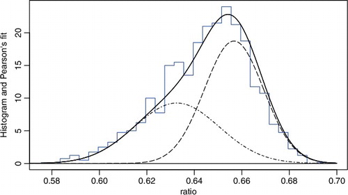
Figure 1 contains, among others, the histogram of a data set containing measurements of 1000 crabs sampled from Bay of Naples provided to Pearson by a biologist (Pearson, 1894). The histogram displays an apparent departure from normality. The departure can be sensibly explained by the possibility that the crab population contains two subpopulations (species). If so, a two-component finite normal mixture model should fit the data well. Indeed, Pearson (1894) found a satisfactory fit via the method of moments to the data set by a finite normal mixture model of order m = 2. We remark that the data can also be well fitted by a Gamma distribution. A finite normal mixture is preferred not for its fit, but for its natural justification.

Figure 1. Histogram of the crab data and the fitted density of two-component normal mixture.

Based on the same interpretation as in Pearson (1894), finite mixture models are routinely used to accommodate the genetic heterogeneity thought to underlie many human diseases. See Chernoff and Lander (1995), Friedlander and Leitersdorf (1995), Schork, Allison, and Thiel (1996) and Ott (1999) for many examples. There are also abundant application examples in Titterington, Smith, and Makov (1985), McLachlan and Peel (2004), and Frühwirth-Schnatter (2006) in other disciplines. We further recommend Lindsay (1995) for some insightful discussions on mixture models.

In addition to their importance in applications, mixture models form a fertile and challenging field of statistical research. The most urgent tasks include point estimation of the mixing distribution G and the related numerical calculation. Interestingly, under mild conditions on {f(x; θ): Θ}, even the nonparametric maximum likelihood estimator (MLE) of G is consistent, given a set of independent and identically distributed (i.i.d. ) observations (Chen, 2016; Kiefer & Wolfowitz, 1956). Geometric properties of the nonparametric MLE were nicely illustrated in Lindsay (1995). These discussions form the solid foundation for numerical computations (Böhning, 2000).

This paper focuses on the hypothesis test problem for order m of the finite mixture model. Due to partial loss of identifiability and its induced non-regularity, the likelihood ratio test (LRT) losses its well-behaved large sample property represented by the famous Wilks theorem (Wilks, 1938). The research activities on this topic may be divided into several stages. Early researchers such as Hartigan (1985) and Ghosh and Sen (1985) revealed the ill effect of the non-regularity. Subsequent research contains rigorous mathematical answers to the asymptotic properties. Some representative results are Chernoff and Lander (1995), Dacunha-Castelle and Gassiat (1999), Liu and Shao (2003) and Chen and Chen (2003). These results are interesting but also conclude that the straightforward LRT is generally impractical. For instance, there are currently no effective numerical methods to evaluate the p-value according to these limiting distributions.

One way to circumvent this obstacle is the famous C(α) test proposed by Neyman and Scott (1965) which is locally optimal and easy to use. However, it is limited to test for homogeneity: namely for H₀: m = 1 when the population contains only one subpopulation. Another line of approach was proposed by Chen (1998) and further developed in Chen, Chen, and Kalbfleisch (2001) and Chen, Chen, and Kalbfleisch (2004). This approach partially restores the regularity through placing a soft bound on mixing proportions. The modified likelihood ratio test (mLRT), as it is now called, leads to Wilks-like asymptotic properties for many but still limited number of commonly used mixture models.

The latest invention, EM-test, enjoys many advantages over the mLRT. When the mLRT works, the EM-test shares its asymptotic properties. The Wilks-like asymptotic properties of the EM-test hold much more broadly. The design of the EM-test comes with many build-in flexibilities. They allow users to utilise features of the specific mixture model to find one version of the EM-test with Wilks-like asymptotic properties. We anticipate advances of the EM-test for multi-parameter mixture models, location-scale mixture models, hidden Markov models (HMMs) and other models with non-i.i.d. data.

This paper is organised as follows. In Section 2, we explain the non-regularity and its implication to classical results on the LRT for homogeneity. Section 3 is devoted to a classical C(α) test for homogeneity. Section 4 contains results on restricted LRT which seem to have limited usage but form a conceptual step-stone for further development. Section 5 presents mLRT and EM-test for homogeneity. Sections 6–8 show how the idea of EM-test is developed to obtain interesting results for the order of finite mixture of single parameter distribution, normal distribution, or data from HMM. We end the paper with some discussions on the future development of the EM-test.

2. Properties of finite mixture models

2.1. Partial identifiability

A parametric model is viable in applications only if it is identifiable. Being identifiable means that for almost all x (with respect to the underlying σ-finite measure) must imply θ₁ = θ₂. A mixture model is identifiable if for almost all x implies G₁ = G₂. We may regard G in (2(2) ) as a functional valued parameter for mixture model (1(1) ). On this platform, most commonly used finite mixture models are identifiable. If G is allowed to be any distribution on Θ, the mixture model (1(1) ) is still identifiable for many important families of f(x; θ).

In applications, our interest goes beyond generic G to include its compositions. Under a finite mixture model, we call m the order of the mixture, π_j the mixing proportions and θ_j the component parameter values of the component distribution f(x; θ). Clearly, we have ∑_jπ_j = 1 and π_j ≥ 0. When any π_j = 0, then the imaginary jth subpopulation does not show up in the mixture. When for some 1 ≤ j₁ ≠ j₂ ≤ m, then these two subpopulations are the same. In both cases, the number of distinct subpopulations is reduced at least by 1 and the model has lost identifiability in this respect. We generally refer them as two types of partial loss of identifiability. They are largely responsible for abnormal asymptotic properties.

2.2. Likelihood ratio test for homogeneity

Let X₁,… , X_n be an i.i.d. sample from a finite mixture model of order m = 2: (3) The problem of testing for homogeneity is specified by two opposing hypotheses (4) LRT for homogeneity is the first choice, but we need a solid statistical foundation.

Let us first consider a simpler and more specific homogeneity problem (Hartigan, 1985): (5) for . Its non-regularity is rooted in the fact that when π = 0, the model becomes a null model for any θ value. In fact, both π and θ only present in H₁, a situation of particular interest (Davies, 1977, 1987).

Under the full model, the log likelihood function is given by where φ(x; μ, σ) is the density function of N(μ, σ²). Define the log likelihood ratio function: Let and . For fixed θ, Y_i(θ) are i.i.d. with zero mean and finite variance σ²(θ) under H₀. Some asymptotic algebra shows that, (6) (7) where is the positive part of for each θ ≠ 0. The leading term in (6(6) ) is a quadratic approximation to the log likelihood ratio function R_n(π; θ).

The authentic LRT statistic for homogeneity without having θ fixed is clearly Over any finite interval, say θ ∈ [0, M] with M < ∞, is easily seen to converge in distribution to a well-defined Gaussian process {Z(θ): 0 ≤ θ ≤ M}. Let θ₁, θ₂,… , θ_K be K arbitrarily selected values in . Then, By choosing sufficiently dispersed θ_j over and large K, we can make arbitrarily large in probability. This leads to the conclusion that R_n → ∞ in probability, a result that bans the use of usual LRT for homogeneity.

The above result does not totally diminish the enthusiasm on LRT for homogeneity. One aberration observed in Hartigan's example can be avoided by placing a compact condition on Θ: |θ| ≤ M < ∞. Under this additional condition, it can be shown that (8) in distribution, a potentially applicable result. At the same time, a rigorous proof of (8(8) ) is not obvious because the quadratic approximation (6(6) ) is valid for each θ ≠ 0, but not uniformly over θ ∈ Θ.

The non-uniformity leads to a technical challenging issue, especially for the original homogeneity problem (4(4) ). To avoid this difficulty, Ghosh and Sen (1985) introduced a separation condition |θ₁ − θ₂| ≥ ε for some ε > 0 in addition to compact constraints |θ₁| ≤ M, |θ₂| ≤ M for (4(4) ). Over the space of (θ₁, θ₂) such that |θ₁ − θ₂| ≥ ε, a uniform quadratic approximation similar to (6(6) ) is obtained. The corresponding LRT statistic was then shown to have a limiting distribution in the familiar form . The Gaussian process Z(θ) and its range are decided by the data-generating distribution f(x; θ₀) and the specific component parameter space Θ.

Subsequent attempts were made to establish the limiting distribution without the separation condition. Chernoff and Lander (1995) were the first to succeed when the component distribution is binomial. Their technique is to transform the parameter space so that the space of H₁ becomes a cone and H₀ becomes a single point on the tip of H₁. Because the component parameter space Θ is naturally compact, they obtained the limiting distribution without placing artificial constraints.

For more general component distribution f(x; θ), Chen and Chen (2001) used a different approach. Similar to Ghosh and Sen (1985), they also obtained a uniform quadratic approximation to the likelihood function over |θ₁ − θ₂| > ε. At the same time, they obtained both lower and upper bounds for the likelihood ratio function over |θ₁ − θ₂| ≤ ε. For finite mixture models of binomial, Poisson, normal with known variance, the difference between the upper and lower bounds reduces to zero as ε → 0. The limit perfectly matches the quadratic approximation obtained earlier when applied to θ₁ = θ₂. Therefore, the LRT statistics indeed has a limiting distribution in the form of . Since the limit at θ₁ = θ₂ is obtained by squeezing two bounds, the technique is named as sandwich method.

Interestingly, for normal mixture model of order m = 2 with structural variance parameter: the limit obtained by sandwich method is stochastically a sum of two independent standard normally distributed random variables. Hence, the limiting distribution of the LRT statistic for homogeneity turns out to have a generic form See Chen and Chen (2003) for details.

Two key intermediate results established in Chen and Chen (2001) are: a uniform quadratic approximation to the likelihood ratio function over |θ₁ − θ₂| > ε, and its smooth limit when ε → 0 coincides with the quadratic approximation within |θ₁ − θ₂| ≤ ε. To some degree, the most general results on homogeneity test and beyond given by Dacunha-Castelle and Gassiat (1999) are obtained by streamline conditions that lead to validity of these two intermediate results.

3. C(α) test for homogeneity

In the past few decades, statisticians succeeded at determining the large sample properties of the LRT statistics. In most cases, these results do not lead to practical homogeneity tests due to numerical difficulty of computing p-values. A C(α) test developed for composite hypotheses by Neyman and Scott (1965) is an attractive alternative.

Consider the situation where an i.i.d. sample from a one-parameter distribution family is available for testing a simple null hypothesis θ = θ₀. When the distribution family is regular, the score function of θ is given by where f′(x; θ) is the derivative of f with respect to θ. It is well known that for any θ. Hence, substantial deviation of S_n(θ₀) from value 0 is an evidence against H₀: θ = θ₀. The degree of deviation is decided by comparing to the reference standard normal distribution where is the Fisher information. Score test as such is known to be locally optimal against one-sided alternative.

Consider now a null hypothesis H₀: θ = θ₀ under a model with multi-parameter θ and ξ. In the presence of nuisance parameter ξ, H₀ is composite such that it contains a set of distributions. We have available two zero-expectation functions: where f′₁ and f′₂ are derivatives with respect to θ and ξ. Since ξ value is not specified under H₀, a root-n consistent estimator will be utilised. The C(α) test seeks a statistic from a linear combination: (9) with a and b chosen by some optimality consideration.

We now discuss how a specific C(α) test is derived for homogeneity in the context of mixture model. Consider the mixture model with density function given by with its parameter space containing all distributions on Θ. We narrow the space down slightly so that all its members have finite second moment. When , we may rewrite the mixture density function as (10) such that the standardised mixing distribution G(·) has mean 0 and variance 1. Under new parameterisation, the null hypothesis becomes H₀: σ = 0. Both θ and the mixing distribution G are nuisance parameters.

The partial derivative of log ϕ(x; θ, σ, G) with respect to σ is given by At σ = 0 or let σ↓0, we find (and define it to be) This is the score function for σ based on a single observation. The choice of is to get a non-degenerate score function.

The partial derivative of log ϕ(x; θ, σ, G) with respect to θ is given by which leads to score function for θ based on a single observation as

We have now identified two zero-expectation functions (under H₀): (11) where x_i's are i.i.d. observations from the mixture model. The score functions based on the entire sample are ∑ⁿ_{i = 1}Z_i(θ) and ∑ⁿ_{i = 1}Y_i(θ) for the mean and variance of G. The optimal combination is given by w_i(θ) = z_i(θ) − β(θ)y_i(θ), with β being the regression coefficient We have capitalised Y and Z to indicate their status as random variables in the above operation. The expectation is with respect to a homogeneous null distribution f(x; θ).

Replacing the unspecified θ by its MLE under homogeneous model f(x, θ), the C(α) statistic arrives at a simple form: (12) with ν(θ) =  E{W²₁(θ)}. Clearly, W_n has standard normal limiting distribution under some general moment conditions on Y and Z. At a given significance level α, we reject the homogeneity hypothesis H₀ when W_n > z_α. This is the C(α) test for homogeneity.

In deriving the C(α) statistic, we assumed that the parameter space . Note that when G(θ) is a mixing distribution on Θ, so is G((θ − θ*)/σ*) for any θ* and σ* ≥ 0. If instead as in the Poisson mixture model in which component distribution has mean θ ≥ 0, G((θ − θ*)/σ*) is not a legitimate mixing distribution for some θ* and σ*. One may re-parameterise the model through ξ = log θ in this case. However, there is no unified approach in general.

Regardless of the hidden validity issue of the mathematical derivation, W_n remains a useful metric on homogeneity hypothesis. Hence, it remains an effective test statistic.

Many commonly used distributions in statistics belong to a group of natural exponential families with quadratic variance function (NEF-QVF; Morris (1982)). The examples include normal, Poisson, binomial, and exponential. The density function in one-parameter natural exponential family has a unified analytical form with respect to some σ-finite measure, where θ = A′(φ) is the mean parameter. Let σ² = A″(φ) be the variance under f(x; θ). To be a member of NEF-QVF, the variance must be a quadratic function of the mean: (13) Take Poisson distribution as an example; it satisfies (13(13) ) with a = 0, b = 1 and c = 0.

C(α) statistic has a particularly simple analytical form under NEF-QVF, where and .

Let X be a random variable with a NEF-QVF mixture distribution and θ be a random variable with distribution G. Denote μ =  E{ E(X|θ)} =  E(θ). When G degenerates, the variance of X is given by σ²(μ) = aμ² + bμ + c. When G does not degenerate, Combining these calculations, we find This inequality shows that the presence of mixture inflates the variance of X by a quantity of size . The test statistic W_n is an over-dispersion measure. Because of this, C(α) test coincides with the detection of over-dispersion in the case of exponential family mixtures.

4. Restricted likelihood ratio test

C(α) test is simple and easy to implement. Yet statisticians are not ready to completely give up the likelihood approach. Many slightly altered likelihood approaches are developed and are effective to some degree. The likelihood method also has potential to test for general order of the mixture model.

As mentioned earlier, there are two types of partial loss of identifiability in the context of homogeneity test. One is when a subpopulation has a very small mixing proportion so that it is practically absent from any sample, the other is when two subpopulations are nearly identical. They are the culprits of the non-standard large sample properties of the LRT. The artificial separation condition is to partly restore regularity to attain some useful results.

Placing a similar condition on mixing proportion is also possible to partly restore the regularity. Chen and Cheng (2000) and Lemdani and Pons (1999) investigated the asymptotic distribution of the LRT under the restriction of min {π₁, π₂} ≥ ε for some ε > 0. Under this restriction, the model defined by (3(3) ) becomes “regular” in some sense.

Assume that we have an i.i.d. sample from (3(3) ). Under mild regularity conditions on component distribution f(x; θ), the MLE of G is consistent (Chen, 2016). The consistency in the functional space is best interpreted as almost surely as the sample size n goes to infinite. This conclusion is not affected when min {π₁, π₂} ≥ ε is applied as long as the true mixing distribution G* satisfies this restriction. When , the consistency leads to (14) This leads to a useful expansion of the log-likelihood function. Let m₁ and m₂ be moments of centred at θ*: By Taylor's expansion, one gets after the high-order terms are ignored.

The further development is algebraically simplest when the random versions of y_i, z_i are uncorrelated. When this is the case, the above expansion leads to Because by definition maximises ℓ_n(G) among all two-point mixing distributions satisfying min {π₁, π₂} ≥ ε, and because of the above expansion, we infer that the moments of must satisfy taking note that m₂ is nonnegative.

Under the null hypothesis that the true mixing distribution G* degenerates, the MLE is searched after under a regular model f(x; θ). We also have with the MLE under the null hypothesis satisfying These informal derivations point to an approximation to the likelihood ratio statistics (under the restriction min {π, 1 − π} > ε > 0) which clearly has a limiting distribution 0.5χ²₀ + 0.5χ₁², the same as in (7(7) ).

This result is mathematically neat because the limiting distribution does not depend on the true distribution θ* nor the choice of ε. It is also easy for numerical computation of the p-value in applications. Nevertheless, the choice of ε is problematic in applications. Its choice affects how well the limiting distribution approximates the finite sample distribution. Our experience indicates that the approximation has poor precision unless ε is somewhat large. Hence, this result is more for insight than of practical value.

5. Modified likelihood ratio test and EM-test for homogeneity

Placing a hard restriction min {π₁, π₂} ≥ ε leads to difficulties at specifying ε in applications. An attractive alternative is developed by placing a soft restriction of similar nature in Chen (1998) and further in Chen et al. (2001), Chen et al. (2004) and others. For test of homogeneity, a modified likelihood as follows is introduced for some positive constant C when G is a mixing distribution with mixing proportions π₁ and π₂. When G degenerates, we use π₁ = π₂ = 0.5 in this definition. When Θ is compact, ℓ_n(G) − ℓ_n(G*) = O_p(1) under some model assumptions. Note that Clog {4π₁π₂} → −∞ when min {π₁, π₂} → 0. Hence, the maximum of is attained at some G with min {π₁, π₂} ≥ c_n > 0. That is, the modified likelihood is an implicitly restricted likelihood. Does it work like a restricted likelihood?

Let be the two support point mixing distribution that maximises the modified likelihood function . Let us define the mLRT statistic to be As shown in Chen et al. (2001), under mild conditions on f(x; θ) and with a compact assumption on Θ, the modified MLE satisfies (15) This mimics (14(14) ) and validates informal expansions that followed. Not surprisingly, in distribution under the null hypothesis. Unlike the restricted LRT, the fitted values of π₁, π₂ in G under modified likelihood are allowed to be arbitrarily close to zero. Hence, the mLRT largely avoids the difficulty to choose an ε.

We seem to merely replace one challenge with another: choosing a properly sized C instead of a properly sized ε. The choice of C is a less touchy issue because it does not lead to direct restrictions on mixing distribution G. The influence of C is mild and smooth on mixing proportions. Chen et al. (2001) found that in most cases, putting C = 1 leads to acceptable precision of the approximation based on limiting distribution 0.5χ²₀ + 0.5χ₁².

In spite of its usefulness as illustrated above, the mLRT exhibits two soft spots. One is that the component parameter space Θ is compact and the other is that Fisher information with respect to mixing proportion for any θ ∈ Θ must be finite. The first requirement is largely ignored in applications and simulation studies such as in Chen et al. (2001). In other words, even though the asymptotic conclusion is possible only if Θ is compact, it matters little in applications.

The second requirement translates into the condition that for any θ ∈ Θ, (16) Consider the finite mixture of exponential distribution where the component density function At homogeneous distribution when θ* = 1, That is, the finite Fisher information condition is violated at θ = 2. Hence, the asymptotic conclusion of the mLRT is not applicable to finite exponential mixture in general. The finite Fisher information condition is also violated for finite mixture of Gamma distributions, of distribution in a scale family, and many more. Unlike the compact condition on Θ, the violation of finite Fisher information condition noticeably changes the asymptotic properties of the mLRT. See Chen and Li (2011) for evidences.

In summary, although the mLRT advances markedly from the original LRT, further development is needed which leads to EM-test. Even though the EM-test and mLRT differ a lot on surface, they are closely connected.

A common thread of the restricted LRT and the mLRT is to apply some constraints to the mixing proportion. Taking the restriction to extreme, let us allow only a few pre-chosen mixing proportions in the space of alternative distributions. This sounds unreasonable, but it is how the EM-test is obtained.

Let X₁,… , X_n be an i.i.d. sample from a two-component finite mixture model (17) the same as before. The log likelihood function under this model assumption is given by (18) Consider the following pair of opposing hypotheses: (19) When H₀ is true and the model f(x; θ) is regular, the statistic has now the typical null limiting distribution (0.5)χ²₀ + (0.5)χ₁². This result does not depend on the specific choice of π = 0.3. We have therefore found a shortcut for homogeneity test: rejecting H₀ when R_n(0.3) is large according to this reference distribution.

Yet, R_n(0.3) has an obvious shortcoming. Suppose the true distribution has two subpopulations with mixing proportions π = 0.16 and 1 − π = 0.84. The most effective test should use R_n(0.16) instead of R_n(0.3). In applications, we do not know the true mixing proportion. To guard against all possibilities, we end up using as the test statistics. However, this statistic is now the LRT statistic, whose distribution was found too difficult to handle.

EM-test breaks this cycle (Li, Chen, & Marriott, 2009) but the strategy and the motivation are somewhat involved. A simplistic and not rigorous version goes as follows. We first specify a mixing proportion for the potential alternative mixture, say π = 0.3,after which, we numerically locate the maximum point of ℓ_n(π; θ₁, θ₂) and denote them as θ⁽⁰⁾₁, θ₂⁽⁰⁾. Given θ⁽⁰⁾₁, θ₂⁽⁰⁾, we locate π⁽⁰⁾ that maximises with some C > 0. Note a regularisation term Clog (1 − |1 − 2π|) slightly different from the one for mLRT is added with a similar purpose. It can be ignored without harming the main line of thinking.

Let G⁽⁰⁾_0.3 be the mixing distribution formed by π⁽⁰⁾, θ⁽⁰⁾₁, θ₂⁽⁰⁾. Applying EM-iteration (Dempster, Laird, & Rubin, 1977) with G⁽⁰⁾ as the initial to obtain G^(K)_0.3 after K iterations. If K → ∞, G^(K)_0.3 converges to at least a local maximum of the log-likelihood function under model (17(17) ). See Wu (1983) for the convergence issue related to EM-algorithm.

To avoid falling back to the LRT statistics, the EM-test constructs a statistic before the iteration converges. For a finite K and given π, define with being the MLE of θ under the null model. Li et al. (2009) found that for each fixed K and J choices of π value, as n → ∞, (20) in distribution. Hence, is a suitable test statistic for homogeneity.

Li et al. (2009) generally recommended to have K = 3 and J = 3 with π taken from {0.1, 0.3, 0.5} in applications. Although EM-iteration for the purpose of computing maximum likelihood estimate is slow, the increment of ℓ_n(G^(k)_π) from k = 0, 1, 2, 3 is mostly in the first two iterations. The change from k = 2 to k = 3 is usually small and the effect on p-value is beyond third decimal place. Further iteration makes little difference. In addition, by iterating from three initial π in {0.1, 0.3, 0.5}, the value of the mixing proportion in G^(k)_π effectively covers the range [0, 0.5]. By symmetry, the range extends to [0, 1]. Hence, increasing the number of initial mixing proportions is not needed.

One may quickly realise that the value of the EM-test statistic is close to a usual LRT statistic, given the same data set. However, EM-test statistic gauges how fast the likelihood increases initially, and the LRT statistic measures how much the likelihood ultimately increases. The advantages of the EM-test include: (a) Θ need not be compact, (b) the second moment as in (16(16) ) need not be finite, (c) much simpler asymptotics, (d) elegant extension to finite normal mixture models (Chen & Li, 2016; Chen, Li, & Fu, 2012).

6. Test for m = m₀ ≥ 2

So far, the discussions are limited to homogeneity test (m = 1) with one-dimensional θ. We now move to H₀: m = m₀ ≥ 2 for one-dimensional θ and for finite normal mixture in both mean and variance.

Consider the one-dimensional θ but general m₀ first. The generic modified likelihood is defined as for G with m support points and mixing proportions π_j. That is, when a model of order m > 2 is fitted to an i.i.d. sample, the likelihood is penalised by Clog π_j for a subpopulation with proportion π_j. Under mild conditions on f(x; θ) and a compact condition on Θ, ℓ_n(G) − ℓ_n(G*) is stochastically bounded as n → ∞, where G* stands for the true distribution. This shows that if maximises among G with m support points, we must have At the same time, the modified MLE is known to be consistent for G* under some conditions, i.e., .

In the context of homogeneity test, the null G* = {θ*} is fitted with a mixing distribution under H₁ and under H₀. Moving from to , 2ℓ_n(G) is increased by {Z⁺(θ*)}² for some standard normal Z. When the null is H₀: m = 2 with we compare the size of ℓ_n(G) maximised over or over directly. From the experience of homogeneity test, we have reason to believe that 2ℓ_n(G) will increase by If Z⁺(θ*₁) and Z⁺(θ*₂) are independent, the limiting distribution would be The truth is more complex but related.

Let  Z = (Z₁, Z₂)^τ and denote its covariance matrix  B. Chen et al. (2004) proved that the mLRT statistic for H₀: m = 2 against H₁: m > 2 after some manipulation asymptotically equals where  t = (t₁, t₂)^τ and  t > 0 is interpreted component-wise. The distribution of this random variable is a mixture of chi-squares where ρ is the correlation coefficient and here π = 3.14159⋅⋅⋅.

EM-test for H₀: m = 2 against H₁: m > 2 has the same limiting distribution and this is not coincident. Unlikely mLRT, EM-test directly specifies a rigid form of mixing distributions permitted in H₁ when maximising in the initial step. Suppose maximises under H₀. Li and Chen (2010) first defined a class of mixing distributions (21) such that for k = 1, 2, each G_k is a mixing distribution of exactly two support points in vicinity of with specific mixing proportions. Among mixing distributions of this form, obtain G⁽⁰⁾ that maximises .

After G⁽⁰⁾ is obtained, EM-iteration is applied K times to get G^(K) as the usual EM-algorithm without restrictions. The meticulously specified G⁽⁰⁾ makes the outcome of the EM-iteration G^(K) retain the form of when H₀ is true. The resultant EM-test statistic therefore has the same limiting distribution as the mLRT.

The advantage is that the EM-test is multiple. It works well with generic m₀. To test H₀: m = m₀ against H₁: m > m₀, the form (21(21) ) is replaced by The EM-test statistic was found to have the same asymptotic expansion: The only difference is the dimensions of  t,  Z and  B. The limiting distribution is a mixture of chi-squares with degrees of freedom ranging from 0 to m₀.

The expansion of the mLRT statistic is established after examining all potential maximisers of the modified likelihood. In comparison, that of the EM-test is established after examining a much reduced class. This key difference leads to simpler technical deliberation and broader applicability of the conclusion. The EM-test does not require compact Θ nor finite Fisher information. The research on the mLRT stopped at H₀: m = 2.

7. EM-test for finite normal mixture model

Two key innovations in developing the EM-test are (a) tactical selection of a special structured class of mixing distributions from H₁ based on the fitted mixing distribution under H₀; (b) use of EM-iteration to measure the improvement in likelihood from H₁ over H₀. These two strategies are broadly applicable. The outcomes are particularly interesting for finite normal mixture models. Let φ(x) be the density function of the standard normal. The density function of a finite normal mixture distribution is given by (22)

Normal mixture distributions are the most important mixture models but their inference is also technically most challenging. The likelihood function of the normal mixture model is unbounded based on a set of random samples, unless an artificial bound is placed on its component variance parameter (Hathaway, 1985). Moreover, the model is not strongly identifiable (Chen, 1995) so it is hard to differentiate between overdispersion caused by mixture or by a large variance. It has infinite Fisher information with respect to mixing proportions. One must regularise the likelihood with some well-designed penalty function to achieve consistent point estimation (Chen, 2016), or settle for restricted MLE (Hathaway, 1985).

Let ℓ_n(G) = ∑log f(x_i; G) still be the log likelihood function given a set of i.i.d. observations from a finite normal mixture distribution and s²_n be the sample variance of x_i, and σ²_j be component variances. One approach to achieve consistent estimation of G is through penalised likelihood defined as for some -dependent smooth penalty function (see Chen, Tan, and Zhang (2008) or Chen (2016)). The key requirement on is that its value goes to negative infinity when σ goes to 0 or infinity at an appropriate rate. One such a choice is The factor a_n determines the level of penalty, and the other factor places a Gamma distribution prior on σ⁻². A recommended choice for a_n is a_n = n^−1/2. As long as a_n > 0, pℓ_n(G) becomes a bounded function of G for each finite m.

The likelihood principle that underlies the hypothesis test is to look for and that maximise the likelihood over spaces of H₀: m = m₀ and H₁: m > m₀, respectively, to form a test statistic. The size reflects the improvement of the fit on H₁ over H₀, and its effectiveness is supported by the classical Neyman--Pearson lemma. At the same time, the test is useful only if asymptotic property of is manageable. In Section 6, we have illustrated that by strategic choice of a subspace of H₁, an EM-test is effective for order of the finite mixture of one-parameter component distribution.

With normal component distribution, Chen et al. (2012) identified a subspace of H₁, made of mixing distributions of order 2m₀ for each carefully selected vector β as follows: (23) where I_j's are non-overlapping intervals containing induced by . For each β, one computes EM-iteration is then applied to pℓ_n(G) with G⁽⁰⁾_β being the initial value to get G^(K)_β, for a pre-specified K. Define The EM-test statistic is defined as the maximum M^(K)_n(β) over a number of carefully selected values of β.

For the ease of presentation, I purposely erred at some details with the general idea preserved. Rigorous readers should consult Chen et al. (2012) for more accurate accounts. Almost like a gift, for testing H₀: m = m₀, in distribution as n → ∞. When the EM-test is applied to Pearson's crab data discussed in the beginning for H₀ of m = 1, 2, the p-values are found to be 8 × 10⁻¹¹ and 0.53, respectively. Hence, an order-2 finite normal mixture model is well supported by the data.

Chen and Li (2016) further studied the order test problem for finite normal mixture model with common component variance: Using the same strategy, an EM-test was constructed and found to have limiting distribution for H₀: m = m₀ when m₀ ≥ 2. Their simulation, however, showed the limiting distribution is not sufficiently accurate for the finite sample distribution. Some additional research is needed.

8. EM-test for hidden Markov model

Under finite mixture models, data X₁, X₂,… , X_n may be regarded as generated in two steps. A hidden variable S_i selects one of m subpopulations with probability π_i in the first step. Given S_i, X_i is a sample from this subpopulation in the second step. The hidden states S₁,… , S_n are themselves i.i.d. 

When S_{1: T} = {S₁, S₂,… , S_T} form a Markov chain instead, the time series X_{1: T} are no longer i.i.d.   However, at equilibrium, the marginal distributions of X_t are identical and have a finite mixture distribution. When S_{1: T} are not observed, the model for X_{1: T} under this formulation is called hidden Markov model (HMM).

In finance applications, market indexes often exhibit distinct stochastic properties over different periods. Such behaviour prompts the suggestion that the stochastic property of related process X_t is determined by some hidden state S_t. A two-state Markov chain for S_{1: T} works well in many specific instances. For example, two states may represent periods of expanding and shrinking economy. Such models are investigated in statistical finance such as Hamilton (2010), Engel (1994) and Chen, Huang, and Wang (2016). At the same time, statistical evidence for the use of multi-state HMM is indispensable.

Consider a simple two-state HMM with state space . At equilibrium, the marginal distribution of X_t has density function (24) where π₁ = P(S_t = 1) and π₂ = P(S_t = 2). The stochastic property of the hidden states S_{1: T} is determined by transition probabilities Because S_{1: T} are generally dependent, so are X_{1: T}. To permit proper equilibrium distribution, the transition probabilities must satisfy certain conditions. When , the HMM has four free parameters: {θ₁, θ₂, p₁₂, p₂₁}. The HMM reduces to a homogenous model when θ₁ = θ₂, or when p₁₂ = 0 or p₂₁ = 0.

The likelihood function of {θ₁, θ₂, p₁₂, p₂₁} may be written as where the summation is over all possible state sequence s_{1: T}, and two extra parameters for the distribution of the initial state S₁: p₁ = 1 − p₂ = P(S₁ = 1).

Interestingly, an easy-to-use forward--backward algorithm is available to compute the MLE of the parameters (Baum, Petrie, Soules, & Weiss, 1970) but evaluating L_n or log L_n is not as straightforward. Full likelihood-based data analysis under HMM is hence challenging in general. One strategy is to replace the likelihood function with a function with similar properties but easier to handle. One such candidate is composite likelihood (CL).

A simplistic introduction of CL is as follows. Additional references can be found in Lindsay (1988), Varin (2008) and Varin, Reid, and Firth (2011). A user may first identify a class of subsets of the observations. A likelihood function can be formed based on each subset of the data under the full model assumption, after which, a log CL is formed as a weighted sum of these log likelihood functions. By a selective choice of these subsets, the CL can be made robust against some degree of model mis-specification, simpler for asymptotic analysis, and easier for numerical computation.

A simple composite log likelihood as the sum of log likelihood based on single x_t is then (25) Note this likelihood has identical algebraic expression when x_{1: T} are T i.i.d.  observations. Hence, all tests discussed under i.i.d. assumptions can be mathematically carried out. Interestingly, the large sample properties of the mLRT and EM-test given in previous sections remain valid. See Dannemann and Holzmann (2008a, 2008b), , Holzmann and Schwaiger (2016) for details. We are saved from adding more details.

9. Future directions

EM-test is currently the most successful approach for testing the order of the finite mixture models. EM-test is a class of tests created based on a conceptually simple principle. They have pushed the boundary of the order test. At the same time, many problems remain unsolved.

There is still lack of effective tests for the order of the finite mixture models with multi-parametric f(x; θ). Within this category, finite mixture of one-dimensional normal distribution is special. Two parameters here specify two distinct aspects of the distribution. EM-test has properly addressed the order test problem in its plain form. At the same time, the EM-test-like solutions often depend on individual features as in Li et al. (2015) and Shen and He (2015). The former deals with the feature where multiple samples are available and the latter works on feature where the mixing proportions are structured.

Finite normal mixture is a special mixture of distributions in a location-scale family. These models are obtained when φ( · ) in (22(22) ) is logistic, Cauchy, Student and so on. Unfortunately, the neat conclusions on the EM-test for normal mixtures are not true. One must start all over again to determine the asymptotic properties of similarly formulated EM-tests. Both interestingly and unfortunately, the large sample properties depend on the specific location-scale family. Some preliminary results obtained by my collaborators indicate that one version of the EM-test for homogeneity of location-scale mixture has limiting distribution assembling (26) with the range on the surface of some three-dimensional cone.

The idea of the EM-test is equally applicable to finite mixture of other generic multi-parameter component distribution (Niu, Li, & Zhang, 2011). The challenge is that the range in the generic (26(26) ) is dependent on the specific model as well as the specific choice of the subspace of H₁. Searching for specific choice that leads to simple limiting distribution is the major task for the future research.

Finally, I wish to turn the attention to non-i.i.d. data such as data from HMM. The EM-test has been found to work well based on CL constructed from marginal distributions as demonstrated by references given earlier. However, this line of approach ignores the time series nature of the HMM. There should be a way to have the transition information accommodated in the EM-test. Finite mixture of regressions forms another rich source of non-i.i.d. data. At this moment, there have been little discussion on tests for the order of regression mixtures.

Acknowledgments

The author likes to thank research fundings from the National Natural Science Foundation of China (Grant No 11690011) and the Natural Science and Engineering Research Council (RGPIN-2014- 03743).

Disclosure statement

No potential conflict of interest was reported by the author.

Additional information

Funding

National Natural Science Foundation of China (Grant No 11690011) and the Natural Science and Engineering Research Council (RGPIN-2014- 03743).

References

- Baum, L. E., Petrie, T., Soules, G., & Weiss, N. (1970). A maximization technique occurring in the statistical analysis of probabilistic functions of Markov chains. The Annals of Mathematical Statistics, 41(1), 164–171.
- Böhning, D. (2000). Computer-assisted analysis of mixtures and applications: Meta-analysis, disease mapping and others. London, UK: Chapman and Hall.
- Chen, H., & Chen, J. (2001). The likelihood ratio test for homogeneity in finite mixture models. Canadian Journal of Statistics, 29(2), 201–215.
- Chen, H., & Chen, J. (2003). Tests for homogeneity in normal mixtures in the presence of a structural parameter. Statistica Sinica, 13, 351–365.
- Chen, H., Chen, J., & Kalbfleisch, J. D. (2001). A modified likelihood ratio test for homogeneity in finite mixture models. Journal of the Royal Statistical Society: Series B, 63(1), 19–29.
- Chen, H., Chen, J., & Kalbfleisch, J. D. (2004). Testing for a finite mixture model with two components. Journal of the Royal Statistical Society: Series B, 66, 95–115.
- Chen, J. (1995). Optimal rate of convergence for finite mixture models. The Annals of Statistics, 23, 221–233.
- Chen, J. (1998). Penalized likelihood-ratio test for finite mixture models with multinomial observations. Canadian Journal of Statistics, 26(4), 583–599.
- Chen, J. (2016). Consistency of the mle under mixture models. Statistical Science. arXiv: 1607.01251.
- Chen, J., & Cheng, P. (2000). The limiting distribution of the restricted likelihood ratio statistic for finite mixture models. Chinese Journal of Applied Probability and Statistics, 2, 159–167.
- Chen, J., Huang, Y., & Wang, P. (2016). Composite likelihood under hidden Markov model. Statistica Sinica, 26(4), 1569–1586.
- Chen, J., & Li, P. (2011). Tuning the em-test for finite mixture models. Canadian Journal of Statistics, 39(3), 389–404.
- Chen, J., & Li, P. (2016). Testing the order of a normal mixture in mean. Communications in Mathematics and Statistics, 4(1), 21–38.
- Chen, J., Li, P., & Fu, Y. (2012). Inference on the order of a normal mixture. Journal of the American Statistical Association, 107(499), 1096–1105.
- Chen, J., Tan, X., & Zhang, R. (2008). Inference for normal mixtures in mean and variance. Statistica Sinica, 18, 443–465.
- Chernoff, H., & Lander, E. (1995). Asymptotic distribution of the likelihood ratio test that a mixture of two binomials is a single binomial. Journal of Statistical Planning and Inference, 43(1), 19–40.
- Dacunha-Castelle, D., & Gassiat, E. (1999). Testing the order of a model using locally conic parametrization: Population mixtures and stationary arma processes. The Annals of Statistics, 27(4), 1178–1209.
- Dannemann, J., & Holzmann, H. (2008a). Likelihood ratio testing for hidden Markov models under non-standard conditions. Scandinavian Journal of Statistics, 35(2), 309–321.
- Dannemann, J., & Holzmann, H. (2008b). Testing for two states in a hidden Markov model. Canadian Journal of Statistics, 36(4), 505–520.
- Davies, R. B. (1977). Hypothesis testing when a nuisance parameter is present only under the alternative. Biometrika, 64(1), 247–254.
- Davies, R. B. (1987). Hypothesis testing when a nuisance parameter is present only under the alternative. Biometrika, 74(1), 33–43.
- Dempster, A. P., Laird, N. M., & Rubin, D. B. (1977). Maximum likelihood from incomplete data via the em algorithm. Journal of the Royal Statistical Society. Series B, 39, 1–38.
- Engel, C. (1994). Can the Markov switching model forecast exchange rates? Journal of International Economics, 36(1–2), 151–165.
- Friedlander, Y., & Leitersdorf, E. (1995). Segregation analysis of plasma lipoprotein (a) levels in pedigrees with molecularly defined familial hypercholesterolemia. Genetic Epidemiology, 12(2), 129–143.
- Frühwirth-Schnatter, S. (2006). Finite mixture and Markov switching models. New York, NY: Springer Science & Business Media.
- Ghosh, J. K., & Sen, P. K. (1985). On the asymptotic performance of the log likelihood ratio statistic for the mixture model and related results. In L. LeCam & R. A. Olshen’ (Eds.), Proceedings of the Berkeley conference in honor of Jerzy Neyman and Jack Kiefer (Vol. 2, pp. 789–806). Belmont, CA: Wadsworth.
- Hamilton, J. D. (2010). Regime switching models. In Macroeconometrics and time series analysis (pp. 202–209). London, UK: Palgrave Macmillan.
- Hartigan, J. A. (1985). A failure of likelihood asymptotics for normal mixtures. In L. LeCam & R. A. Olshen’ (Eds.), Proceedings of the Berkeley conference in honor of Jerzy Neyman and Jack Kiefer (Vol. 2, pp. 807–810). Belmont, CA: Wadsworth.
- Hathaway, R. J. (1985). A constrained formulation of maximum-likelihood estimation for normal mixture distributions. The Annals of Statistics, 13, 795–800.
- Holzmann, H., & Schwaiger, F. (2016). Testing for the number of states in hidden Markov models. Computational Statistics and Data Analysis, 100, 318–330.
- Kiefer, J., & Wolfowitz, J. (1956). Consistency of the maximum likelihood estimator in the presence of infinitely many incidental parameters. The Annals of Mathematical Statistics, 27, 887–906.
- Lemdani, M., & Pons, O. (1999). Likelihood ratio tests in contamination models. Bernoulli, 5(4), 705–719.
- Li, P., & Chen, J. (2010). Testing the order of a finite mixture. Journal of the American Statistical Association, 105(491), 1084–1092.
- Li, P., Chen, J., & Marriott, P. (2009). Non-finite fisher information and homogeneity: An EM approach. Biometrika, 96, 411–426.
- Li, S., Chen, J., Guo, J., Jing, B.-Y., Tsang, S.-Y., & Xue, H. (2015). Likelihood ratio test for multi-sample mixture model and its application to genetic imprinting. Journal of the American Statistical Association, 110(510), 867–877.
- Lindsay, B. G. (1988). Composite likelihood methods. Contemporary Mathematics, 80(1), 221–239.
- Lindsay, B. G. (1995). Mixture models: Theory, geometry and applications. In NSF-CBMS regional conference series in probability and statistics. Hayward, CA: Institute of Mathematical Statistics.
- Liu, X., & Shao, Y. (2003). Asymptotics for likelihood ratio tests under loss of identifiability. Annals of Statistics, 31, 807–832.
- McLachlan, G., & Peel, D. (2004). Finite mixture models. New York, NY: John Wiley & Sons.
- Morris, C. N. (1982). Natural exponential families with quadratic variance functions. The Annals of Statistics, 10, 65–80.
- Neyman, J., & Scott, E. (1965). On the use of c (alpha) optimal tests of composite hypotheses. Bulletin of the International Statistical Institute, 41(1), 477–497.
- Niu, X., Li, P., & Zhang, P. (2011). Testing homogeneity in a multivariate mixture model. Canadian Journal of Statistics, 39(2), 218–238.
- Ott, J. (1999). Analysis of human genetic linkage. Baltimore, MD: JHU Press.
- Pearson, K. (1894). Contributions to the mathematical theory of evolution. Philosophical Transactions of the Royal Society of London A, 185, 71–110.
- Schork, N. J., Allison, D. B., & Thiel, B. (1996). Mixture distributions in human genetics research. Statistical Methods in Medical Research, 5(2), 155–178.
- Shen, J., & He, X. (2015). Inference for subgroup analysis with a structured logistic-normal mixture model. Journal of the American Statistical Association, 110(509), 303–312.
- Titterington, D. M., Smith, A. F., & Makov, U. E. (1985). Statistical analysis of finite mixture distributions. New York, NY: Wiley.
- Varin, C. (2008). On composite marginal likelihoods. AStA – Advances in Statistical Analysis, 92(1), 1–28.
- Varin, C., Reid, N., & Firth, D. (2011). An overview of composite likelihood methods. Statistica Sinica, 21, 5–42.
- Wilks, S. S. (1938). The large-sample distribution of the likelihood ratio for testing composite hypotheses. The Annals of Mathematical Statistics, 9(1), 60–62.
- Wu, C. J. (1983). On the convergence properties of the em algorithm. The Annals of statistics, 11, 95–103.