Personalised treatment assignment maximising expected benefit with smooth hinge loss

ABSTRACT

In personalised medicine, the goal is to make a treatment recommendation for each patient with a given set of covariates to maximise the treatment benefit measured by patient's response to the treatment. In application, such a treatment assignment rule is constructed using a sample training data consisting of patients’ responses and covariates. Instead of modelling responses using treatments and covariates, an alternative approach is maximising a response-weighted target function whose value directly reflects the effectiveness of treatment assignments. Since the target function involves a loss function, efforts have been made recently on the choice of the loss function to ensure a computationally feasible and theoretically sound solution. We propose to use a smooth hinge loss function so that the target function is convex and differentiable, which possesses good asymptotic properties and numerical advantages. To further simplify the computation and interpretability, we focus on the rules that are linear functions of covariates and discuss their asymptotic properties. We also examine the performances of our method with simulation studies and real data analysis.

KEYWORDS:

• Convex loss
• linear rules
• oracle property
• subgroup identification
• weighted outcome learning

1. Introduction

Differential treatment effects are common in many diseases, because patients with different covariates, such as demographics, genomic information, treatment and outcome history, may not respond to treatments homogeneously. For example, molecularly targeted cancer drugs are mostly effective for patients with tumours expressing the targets (Lee et al., 2016; Ulloa-Montoya et al., 2013; Zhao et al., 2016). Significant heterogeneity exists in responses among patients with different baseline levels of psychiatric symptoms (Crits-Christoph et al., 1999; Kessler et al., 2016). Personalised medicine accounts for individual heterogeneity by constructing a treatment assignment rule as a function of patient covariates to maximise the treatment benefit measured by patient's response to the treatment. Thus, it has gained considerable popularity in clinical practice and medical research in recent years.

Typically, a treatment assignment rule is built based on a training data set consisting of patients’ responses and covariates from a medical or clinical study. One statistical approach that has long been discussed and explored is to fit a model based on patient's response, covariates and treatment received, since the expected patient's benefit is usually related to some characteristics under this model, e.g., the conditional expectation of patient's response given the covariates and treatment. Because this approach largely depends on the model, misspecification of the model leads to unreliable treatment assignment. This issue becomes even more prominent when the number of covariates is large, which is often the case in clinical trials and medical research. In addition, different types of data, e.g., binary, continuous, time-to-event, and possibly mixed outcomes, have to be dealt with differently in this approach.

An alternative approach circumvents the need for outcome model specification by directly searching an assignment rule that maximises the expected patient's benefit (Zhao, Zeng, Rush, & Kosorok, 2012). This approach uses patients’ responses (of any type) as weights in a target function that is related to patient's benefit as well as treatment-covariate interaction effects. Instead of using the zero–one loss in the target function, which is natural but hard or impossible for numerical implementation, efforts have been made by researchers in search of a surrogate loss function for the zero–one loss that can be easily implemented and leads to solutions with good properties; for example, the hinge loss considered by Zhao et al. (2012) and the logistic loss used by Xu et al. (2015). Unlike the zero–one loss, the hinge loss is convex and continuous, but not differentiable so that numerical optimisation under the hinge loss requires some additional techniques. Although the logistic loss is convex, differentiable, and simple for optimisation, unlike the hinge loss, it does not produce a solution that is exactly the same as the solution under the zero–one loss.

The purpose of our study is to propose a sequence of convex and differentiable functions as the surrogate loss functions in applying the previously described direct searching approach. Since the limit of this sequence of loss functions is the hinge loss function and each function in this sequence has a hinge shape, we call these functions the smooth hinge loss functions. A detailed description of the target function and related loss functions are given in Section 2, where we also establish the equivalence of the optimal treatment assignment rule under the zero–one loss and hinge loss, and show that we may focus on rules linear in covariates under some conditions. An advantage of considering rules linear in covariates is that they are simple to compute and easy to interpret. In Section 3, we introduce the smooth hinge loss and our methodology. To address high covariate dimension issue, we propose to add a LASSO penalty in the optimisation under the smooth hinge loss. Some asymptotic properties of our solution are established. Numerical performance of our approach is examined by simulation in Section 4. Section 5 contains an example. All technical proofs are given in the Appendix.

2. Target function, hinge loss, and linear rules

Let T ∈ {−1, 1} be a binary treatment with P(T = 1) = π, 0 < π < 1, Y be a univariate patient's response, and X be a p-dimensional covariate vector including interactions and dummy variables for categorical covariates. We focus on the case where X and T are independent, e.g., a randomised trial. Let D(X) be a treatment assignment rule as a function of X, P be the joint distribution of (Y, T, X), and P^D be the conditional distribution of (Y, T, X) given T = D(X). Then, the expected outcome under rule D is given by (Qian & Murphy, 2011) where I{A} is the indicator function of a set A. Assume that a large Y is preferable and Y is bounded. Then, E^D(Y) is the expected patient's benefit under zero–one loss and assignment rule D. Our goal is to assign each patient a treatment based on X to maximise E^D(Y). Hence, we aim to find the optimal rule D^* that (1) where is the set of all Borel functions of X with range {−1, 1}. Note that D^*(X) does not change if Y is replaced by Y + c for any constant c. We assume Y ≥ 0.

Due to the discontinuity and nonconvexity of the zero–one loss (the indicator function), it is difficult to empirically perform the minimisation in (1(1) ). A common practice to mitigate this problem is to use a continuous and convex surrogate loss. Adopting the hinge loss as a surrogate loss, Zhao et al. (2012) proved that if (2) where (1 − a)⁺ = (1 − a)I{a ≤ 1} and is the set of all Borel functions, then D^*(X) = sign{f^*(X)} a.s. We establish a stronger result as the following proposition. Its proof is given in the Appendix.

Proposition 2.1:

Let D^* and f^* be given by (1(1) ) and (2(2) ), respectively. Then, f^*(X) = D^*(X) a.s.

In general, the optimal rule D^*(X) could be a complicated function of X. The following proposition shows that under a mild condition, D^*(X) only depends on the sign of a linear function of X. This is a slightly modified version of Proposition 1 in Xu et al. (2015). Throughout the paper, a′ denotes the transpose of a vector a.

Proposition 2.2:

Suppose that (3) where β^† is a p-dimensional vector, l(X) is a function of X, and g(a, b) is a bivariate function satisfying g(a, b) ≥ g(a, −b) if b ≥ 0 any real valued a. Then, D^*(X) = sign(X′β^†) a.s.

Since β^† and functions l and g can all be unknown, many useful models in application satisfy (3(3) ).

With the hinge loss, can we perform the minimisation in (2(2) ) by focusing on linear functions of X? That is, if (4) can we conclude that f^*(X) = sign(X′β^*)? In general, the answer is no, because Propositions 1 and 2 imply that D^*(X) = f^*(X) = sign(X′β^†), which does not necessarily imply f^*(X) = sign(X′β^*). But the following result indicates that D^*(X) = f^*(X) = sign(X′β^*) holds under some conditions. The proof is in the Appendix.

Proposition 2.3:

Suppose that (3(3) ) holds and that (5) where c_β is a constant that depends on β. Let φ be a continuous and convex function satisfying (6) for any real valued w and z and any c > 0. Then, there exist and such that .

For the hinge loss φ(z) = (1 − z)⁺, condition (6(6) ) is satisfied. Hence, f^*(X) = sign(X′β^*) if condition (5(5) ) holds. Li (1991) proved that condition (5(5) ) is satisfied when the distribution of X is elliptically symmetric, e.g., X is multivariate normal.

The conclusion is that the hinge loss is a good surrogate for the zero–one loss and, under condition (5(5) ), we can focus on linear functions of X in the minimisation in (2(2) ).

3. Smooth hinge loss and optimal linear rule

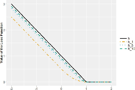
Unfortunately, if we focus on linear rules, solving the minimisation problem (4(4) ) empirically is still difficult, because hinge loss is not always differentiable. We therefore propose to use a differentiable loss function to establish desirable asymptotic properties, as well as enhancing computational performance. We consider the following smooth hinge loss introduced by Rennie (2005): (7) where k ≥ 1 is an integer. The smooth hinge loss is twice differentiable for every k. For a fixed z, the smooth hinge loss function increases with k, and converges to the hinge loss function as k goes to infinity. Figure 1 shows the hinge loss and the smooth hinge loss with k = 1, 5, and 10.

Figure 1. Hinge loss h and smooth hinge loss h_k.

With the smooth hinge loss being a surrogate loss, we focus on the optimisation problem (8) The following proposition shows that, as k → ∞, the minimum of the risk function with smooth hinge loss (achieved at β*_k) converges to the minimum of the risk function with hinge loss (achieved at β^*). Furthermore, with the hinge loss, the risk function at β*_k converges to the minimum of the risk function. The proof is in the Appendix.

Proposition 3.1:

Define and to be the risk functions for the hinge loss and smooth hinge loss h_k, respectively. Then,

In application, we can solve (8(8) ) with the expectation replaced by the sample average based on an independent sample (Y_i, T_i, X_i), i = 1,… , n, identically distributed as (Y, T, X). To perform variable selection, we add the LASSO penalty and solve

(9) where ‖β‖₁ is the L₁ norm of β, λ_n is a LASSO tuning parameter, and is the proportion of treatment group subjects in the data set. We define the final empirical treatment assignment rule as . Because a smooth hinge loss is used as the surrogate loss, we name this method as the sHinge method.

In the rest of this section, we show that possesses a weak oracle property. We need some notations. For any β, let be the index set of non-zero components of β, where β_(j) is the jth component of β. Let β*^I_k be the subvector of β*_k with indices in , X_I be the subvector of X with indices in , and X₀ be the subvector of X with components not in X_I. Let s_p be the cardinality of and be the minimal signal. For any a = (a₍₁₎,… , a_(q)), let ‖a‖_∞ = max _{j ≤ q}|a_(j)|. For any two sequence a_n and b_n, a_n ≈ b_n denotes a_n = O(b_n) and b_n = O(a_n). Without loss of generality, we assume E(X) = 0.

The proof of the following result is in the Appendix.

Theorem 3.1

(Weak oracle property): Assume that the following conditions hold.

(C1) for any t, where c is a constant and X_(j) is the jth component of X.

(C2) 0 ≤ Y ≤ M with a constant M.

(C3) , , and , where α_s, α_p, and α_d are constants satisfying 0 < α_s < γ < α_p < 1/2 and 0 < α_d < γ for a constant γ > 0.

(C4) and , where b_n = o(n^{1/2 − γ}/(log n)^1/2), , is the second-order derivative of h_k(x), and W = Y/{Tπ + (1 − T)/2}.

(C5) k ≈ n^ξ with a constant ξ < γ − α_s.

If we choose λ_n such that (10) then, when n is sufficiently large, with probability greater than , there exists a satisfying (9(9) ) and

(a) (sparsity) ;

(b) (L_∞ consistency) .

From Theorem 3.1, we know that under certain conditions, as n, p and k diverge to infinity in a certain way, with probability converging to one, correctly identifies all the zero components of β*_k and estimates the non-zero components of β*_k consistently in the rate n^−γ. In other words, the penalised empirical solution is a good estimate of the theoretical optimiser β*_k, in the sense of weak oracle property. Furthermore, with the risk for the hinge loss, it follows from Theorem 3.1 and Proposition 3.1 that is risk-consistent.

Corollary 3.1:

Under the conditions of Theorem 3.1, converges to R(β^*) in probability as n → ∞.

4. Simulation results

In this section, we compare by simulation the proposed sHinge method with the ROWSi method in Xu et al. (2015), which solves (9(9) ) with h_k replaced by the logistic loss φ(t) = log (1 + e^−t). The reason why we compare our sHinge method with the ROWSi is that Xu et al. (2015) showed by simulation that the ROWSi was superior over the method solving (9(9) ) with h_k replaced by the hinge loss, which was proposed in Zhao et al. (2012) except that LASSO penalty instead of L₂ penalty was used for variable selection. Xu et al. (2015) also showed by simulation that ROWSi was superior over other four recently proposed methods, the interaction tree by Su, Tsai, Wang, Nickerson, and Li (2009), the virtual twins by Foster, Taylor, and Ruberg (2011), the logistic regression with LASSO penalty by Qian and Murphy (2011), and the FindIt by Imai and Ratkovic (2013).

For our method, was computed by optimising the target function in (9(9) ) with coordinate descent algorithm (Friedman, Hastie, Höfling, & Tibshirani, 2007). The parameter k in h_k was set to be 2 in all the settings. To implement ROWSi, we used the R codes provided by the authors, in which a group LASSO procedure was used to pre-screen the interaction terms. For both methods, we chose the tuning parameter λ by a 10-fold cross-validation. The criterion used in validation was the prediction accuracy, which is defined as the proportion of empirical treatment assignments that are consistent with the oracle assignments sign(x′β^†) (Xu et al., 2015).

We considered three types of covariates: binary covariates (X_A, X_B, X_C, …), discrete covariates (X_a, X_b, X_c, …) with four categories, and continuous covariates (X_Ca, X_Cb, X_Cc, …). Deviation coding was used for all discrete covariates: a binary X_A was coded as ±1 and a X_a with four categories was coded as

Table

	Coded variables
Xa	Xa1	Xa2	Xa3
1	1	0	0
2	0	1	0
3	0	0	1
4	−1	−1	−1

All discrete covariates were simulated from the uniform distribution over their categories and all continuous covariates were simulated from the standard normal distribution. All covariates were generated independently. The treatment T takes values ±1 with equal probability and is independent of the covariates. We considered the following eight models between a binary response Y and (covariates, treatment) with up to three-way interactions among treatment and covariates. In the following, ε denotes a standard normal random variable independent of treatment and all covariates, and I{A} denotes the indicator function of set A.

I.	X = (Xa, Xb, XA, XB, XCa, XCb) and
II.	X = (Xa, Xb, XA, XB, XCa, XCb) and
III.	X = (Xa, Xb, Xc, XA, XB, XC, XCa, XCb, XCc) but Y is the same as that in (I), i.e., covariates Xc, XC, and XCc are actually not related with Y.
IV.	X = (Xa, Xb, Xc, XA, XB, XC, XCa, XCb, XCc) but Y is the same as that in (II), i.e., covariates Xc, XC, and XCc are actually not related with Y.
V.	X = (Xa, Xb, Xc, Xd, Xe, XA, XB, XC, XD, XE, XCa) and
VI.	X = (Xa, Xb, Xc, Xd, Xe, XA, XB, XC, XD, XE, XCa) and
VII.	X = (XCa, XCb, XCc, XCd, XCe, XCf, XCg, XCh) and
VIII.	X = (XCa, XCb, XCc, XCd, XCe, XCf, XCg, XCh) and

In settings II, IV, VI and VIII, Y follows a logistic model. In settings I, III, V and VII, Y is an indicator of a regression; in these models, the conditions in Proposition 2.2 are violated. The purpose of including them was to test the robustness of the methods. In settings I and II, all covariates show up in the model, whereas in settings III and IV, one of three types of covariates is not related with Y. Models in V and VI contain only one continuous covariate and discrete covariates are dominant in the interaction terms. The last two models contain only continuous variables.

For each setting, three sample sizes, n = 500, 1000 and 1500, were used and the number of simulation runs was 200.

We evaluated the performances of both methods by three criteria: sensitivity, specificity and prediction accuracy. Sensitivity is defined as the proportion of true non-zero interactions being estimated as non-zero. Specificity is defined as the proportion of true zero interactions being estimated as zero. Prediction accuracy follows the definition in the discussion of the cross-validation procedure.

To compare the ability of variable selection, Figures 2 and 3 show sensitivity and specificity, respectively, based on 200 simulations. Both methods demonstrated exceptional ability to identify non-zero interaction terms, as shown in Figure 2. When the sample size is large, the sensitivity can even reach 1, meaning that all non-zero components are successfully identified. Figure 3 indicates that our method greatly surpasses ROWSi in the ability to identify unimportant interaction terms. The performance of our method is shown to be stable across different sample sizes, while ROWSi has exhibited a decreasing trend in specificity as the sample size increases, which indicates that ROWSi may not have the consistency property described in our Theorem 3.1.

Figure 2. Comparison of sensitivity (sHinge vs. ROWSi).

Figure 3. Comparison of specificity (sHinge vs. ROWSi).

As for prediction accuracy, as shown in Figure 4, our method again excels ROWSi in almost all settings. The only exceptions are settings V and VI with n = 500, where the prediction accuracy of our method is lower by a small amount no larger than 0.0083.

Figure 4. Comparison of prediction accuracy (sHinge vs. ROWSi).

5. Example

In this section, we apply our proposed method to a real data set from a large randomised trial that evaluates the efficacy of the telephone intervention at promoting mammography screening for women who were 51–75 years of age but non-adherent to breast cancer screening guidelines at baseline (Champion et al., 2016). The original study has three arms. We consider two arms that consist of 574 subjects in the phone intervention group and 544 in the usual care (control) group. The primary outcome of interest Y is a binary variable for mammography screening (1 = yes, 0 = no) at 21 months post-baseline. The covariate vector X consists of 21 covariates, of which 16 are binary, one is categorical, and four are numerical. The covariates names and descriptions are listed in Table 1.

Table 1. Variables in the mammography screening data set.

resp21	Mammography screening 21 months post-baseline (yes/no)
treatment	1 = phone, −1 = control
age	Age
educyrs	Years of education
collegeormore	Four-year college or more (yes/no)
raceaa	African American (yes/no)
married	Married or in long-term relationship (yes/no)
income3	Household income (1 ≤ 30 K, 2 = 30–75 K, 3 ≥ 75 K)
workpay	Currently working for pay (yes/no)
stgpca1	Baseline stage of behaviour change, 0 = precontemplation (not planning), 1 = contemplation (planning)
mediapaper	Exposure to paper media (yes/no)
mediatv	Exposure to TV media (yes/no)
mediainternet	Exposure to Internet media (yes/no)
hadmamm1	Ever had a mammogram (yes/no)
yearmamsum	Number of years had a mammogram in the past 2–5 years
doceversug	Doctor ever suggest you have a mammogram (yes/no)
docspoke	Doctor/nurse spoke to you in the last 2 years about mammogram (yes/no)
famhist	Family history of breast cancer (yes/no)
hcreminder	Received reminders of mammogram from a health care facility (yes/no)

We intended to apply our method to obtain with given by (9(9) ), which determines the subgroup of subjects that would benefit from the phone intervention. However, the Y values were missing for 122 subjects. Assuming that missingness depends on covariates, we imposed a weight to each observed Y value and solved a modified version of (9(9) ):

(11)

where , h₁ is the smooth hinge loss with parameter k = 1, is the proportion of treatment group subjects in the data set, is an estimate of the propensity P(Y_i is observed|X_i) given by with The tuning parameters λ_n and υ_n were selected by five-fold cross-validation with BIC being the criterion.

The resulting assignment rule is This indicates that, for mammography screening, women who are non-adherent to breast cancer screening guidelines will benefit more from the phone intervention if they are

• in an older age group,

• had fewer years of education.

We also applied the ROWSi method in Xu et al. (2015), which simply replaces the loss function h₁(·) in (11(11) ) by the logistic loss log (1 + exp (·)). However, it failed to select any covariates, i.e., it assigned all the subjects to the control group.

Acknowledgments

The views in this publication are solely the responsibility of the authors and do not necessarily represent the views of the Patient-Centered Outcomes Research Institute (PCORI), its Board of Governors or Methodology Committee.

Disclosure statement

No potential conflict of interest was reported by the authors.

Additional information

Funding

Research reported in this article was partially funded through a Patient-Centered Outcomes Research Institute (PCORI) Award [ME-1409-21219]. The second author's research was also partially supported by the Chinese 111 Project [B14019] and the US National Science Foundation [grant number DMS-1612873].

Appendix

Proof of Proposition 2.1

For a.s. any fixed x, Then, for f such that f(x) ≥ 1, (A1) For f such that f(x) ≤ −1, (A2) For f such that −1 < f(x) < 1, (A3)

The minimum of (A1(A1) ) is = 2E(Y|X = x, T = −1), obtained at f such that f(x) = 1. The minimum of (A2(A2) ) is = 2E(Y|X = x, T = 1), obtained at f such that f(x) = −1. When , the minimum of (A3(A3) ) is 2E(Y|X = x, T = −1) obtained at f such that f(x) = 1. When , the minimum of (A3(A3) ) is 2E(Y|X = x, T = 1) obtained at f such that f(x) = −1. Also, notice that when , the minimum of (A1(A1) ) is smaller than the minimum of (A2(A2) ), and when , the minimum of (A2(A2) ) is smaller than the minimum of (A1(A1) ). Therefore, Hence, for a.s. any fixed x.

Proof of Proposition 2.3

For any β, where the fifth equality follows from the independence of T and X, the inequality is the result of an application of Jensen's inequality with conditional expectation, and the last equality follows from condition (5(5) ). Similarly, we can show that Thus, for any β, Suppose that the minimum on the far right side of the previous expression is achieved at . By definition, . It remains to prove that . This follows because for any c > 0, by condition (6(6) ).

Proof of Proposition 3.1

By the definition, and β^* = argmin_βR(β). From we obtain that and for any β, Hence, as k → ∞, i.e., R_k converges to R uniformly in β. Then, by the definition of β^*. On the other hand, by the definition of β*_k, This proves lim_{k → ∞}R_k(β*_k) = R(β*), which is the first conclusion. From the uniform convergence, lim_{k → ∞}[R_k(β*_k) − R(β*_k)] = 0. This together with the first conclusion proves the second conclusion lim_{k → ∞}R(β*_k) = R(β*).

Proof of Theorem 3.1

Let p₁(β) = ∑^p_{j = 1}|β_(j)|. Then, the subgradient of p₁(β) is ∂p₁(β_(j)), a set-valued function such that (A4) By the classical optimisation theory, the KKT condition is (A5) where s_j ∈ ∂p₁(β_(j)), , , is a function from to such that its ith element is , is the first-order derivative of h_k, and ○ denotes componentwise product. Then, any vector satisfying the following KKT conditions is a solution to (9(9) ): (A6) (A7) where is the submatrix of with columns in and is the submatrix of with columns not in , and β^I is the subvector of β with indices in .

In the following, we show that within a neighbourhood of β*_k, a vector satisfying the KKT conditions exists and it also satisfies conclusions (a) and (b) in Theorem 3.1. Define and events where C₁ and C₂ are constants depending on c and M. Let ε_j be the jth component of . Under conditions (C1) and (C2), ε_j is sub-Gaussian, i.e., there exists a constant c₁ depending on c and M that By the Hoeffding's bound for sub-Gaussian random variables, it holds that Let , it follows from Bonferroni inequality that Similarly, we can show that Since |μ(x)| ≤ 1, following the same technique, we can show that Therefore, Next, we show that within event E₁∩E₂∩E₃∩E₄, there exists a solution to (A6(A6) ) and (A7(A7) ), and it satisfies (a) and (b). First, we prove that, when n is sufficiently large, there exists a solution to (A6(A6) ) in the hypercube Since and which is integrable, it follows that (A8) Then, the condition in (A6(A6) ) is equivalent to or where . By Taylor expansion, where lies on the line segment connecting δ and β*^I_k and the fact that T² = 1 is used. Thus, (A6(A6) ) is equivalent to or , where Since , (C4) implies that With the choice of λ_n, it follows that Then, for sufficiently large n, if δ_j − β*_{k, (j)} = n^{− γ}, ; if δ_j − β*_{k, (j)} = −n^{− γ}, . By continuity of Ψ(δ), an application of Miranda's existence theorem shows that has a solution in , which is also a solution to (A6(A6) ). Denote this solution by . Let . Then, satisfies (a) by definition.

Next, we prove that satisfies (A7(A7) ) and (b). By (A8(A8) ), Then, (A9) By Taylor expansion, (A10) where lies on the line segment connecting and β*^I_k. Since is the solution to , it holds that (A11) So satisfies (b); that is, . By (A9(A9) ), (A10(A10) ) and (A11(A11) ), In the event E₁∩E₂∩E₃∩E₄, by the choice of λ_n, Note that . (C4) indicates that Finally, again by (C4), Therefore, satisfies (A7(A7) ). This completes the proof.

Proof of Corollary 3.1

The result follows from Theorem 3.1, the dominated convergence theorem under (C1) and (C2), and Proposition 3.1.

References

- Champion, V. L., Rawl, S. M., Bourff, S. A., Champion, K. M., Smith, L. G., Buchanan, A. H., … Skinner, C. S. (2016). Randomized trial of dvd, telephone, and usual care for increasing mammography adherence. Journal of Health Psychology, 21, 916–926.
- Crits-Christoph, P., Siqueland, L., Blaine, J., Frank, A., Luborsky, L. S., Onken, L. S., … Beck, A. T. (1999). Psychosocial treatments for cocaine dependence. Archives of General Psychiatry, 56, 493–502.
- Foster, J., Taylor, J., & Ruberg, S. (2011). Subgroup identification from randomized clinical trial data. Statistics in Medicine, 30, 2867–2880.
- Friedman, J., Hastie, T., Höfling, H., & Tibshirani, R. (2007). Pathwise coordinate optimization. Annals of Applied Statistics, 1, 302–332.
- Imai, K., & Ratkovic, M. (2013). Estimating treatment effect heterogeneity in randomized program evaluation. The Annals of Applied Statistics, 7, 443–470.
- Kessler, R. C., van Loo, H. M., Wardenaar, K. J., Bossarte, R. M., Brenner, L. A., Ebert, D. D., … Zaslavsky, A. M. (2016). Using patient self-reports to study heterogeneity of treatment effects in major depressive disorder. Epidemiology and Psychiatric Sciences, 26, 22–36.
- Lee, C. K., Davies, L., Gebski, V. J., Lord, S. J., Di Leo, A., Johnston, S., … de Souza, P. (2016). Serum human epidermal growth factor 2 extracellular domain as a predictive biomarker for lapatinib treatment efficacy in patients with advanced breast cancer. Journal of Clinical Oncology, 34, 936–944.
- Li, K.-C. (1991). Sliced inverse regression for dimension reduction. Journal of the American Statistical Association, 86, 316–327.
- Qian, M., & Murphy, S. A. (2011). Performance guarantees for individualized treatment rules. The Annals of Statistics, 39, 1180–1210.
- Rennie, J. D. M. (2005). Smooth hinge classification. Retrieved from http://people.csail.mit.edu/jrennie/writing
- Su, X., Tsai, C.-L., Wang, H., Nickerson, D., & Li, B. (2009). Subgroup analysis via recursive partitioning. Journal of Machine Learning Research, 10, 141–158.
- Ulloa-Montoya, F., Louahed, J., Dizier, B., Gruselle, O., Spiessens, B., Lehmann, F. F., … Brichard, V. G. (2013). Predictive gene signature in mage-a3 antigen-specific cancer immunotherapy. Journal of Clinical Oncology, 31, 2388–2395.
- Xu, Y., Yu, M., Zhao, Y.-Q., Li, Q., Wang, S., & Shao, J. (2015). Regularized outcome weighted subgroup identification for differential treatment effects. Biometrics, 71, 645–653.
- Zhao, S. G., Chang, S. L., Spratt, D. E., Erho, N., Yu, M., Ashab, H. A.-D., … Feng, F. Y. (2016). Development and validation of a 24-gene predictor of response to postoperative radiotherapy in prostate cancer: A matched, retrospective analysis. The Lancet Oncology, 17, 1612–1620.
- Zhao, Y., Zeng, D., Rush, A. J., & Kosorok, M. R. (2012). Estimating individualized treatment rules using outcome weighted learning. Journal of the American Statistical Association, 107, 1106–1118.