Cholesky-based model averaging for covariance matrix estimation

ABSTRACT

Estimation of large covariance matrices is of great importance in multivariate analysis. The modified Cholesky decomposition is a commonly used technique in covariance matrix estimation given a specific order of variables. However, information on the order of variables is often unknown, or cannot be reasonably assumed in practice. In this work, we propose a Cholesky-based model averaging approach of covariance matrix estimation for high dimensional data with proper regularisation imposed on the Cholesky factor matrix. The proposed method not only guarantees the positive definiteness of the covariance matrix estimate, but also is applicable in general situations without the order of variables being pre-specified. Numerical simulations are conducted to evaluate the performance of the proposed method in comparison with several other covariance matrix estimates. The advantage of our proposed method is further illustrated by a real case study of equity portfolio allocation.

Keywords:

• High-dimension
• ensemble estimate
• Cholesky factor
• positive definite
• portfolio strategy

1. Introduction

Estimation of a covariance matrix from a sample of multivariate data is of great importance. The sample covariance matrix estimate becomes less attractive with the increase of the number of variables. In many applications such as gene expression, fMRI, spectroscopic imaging and weather forecasting, the number of variables largely exceeds the sample size. In this situation, the sample covariance matrix has a distorted eigen-structure (Johnstone, 2001). Therefore, it is important to explore appropriate covariance matrix estimation in large dimension cases.

A natural way of improving covariance matrix estimation is to modify the sample covariance matrix. Ledoit and Wolf (2004) considered a Steinian estimate that shrinks the sample covariance matrix towards the identity matrix. The eigenvalues of their estimate are weighted averages of the ones from the sample covariance matrix and the identity matrix. Quite often, the small eigenvalues of their estimate are exaggerated. Another approach is to focus on regularising the sample covariance matrix. Bickel and Levina (2008a) considered thresholding small entries of the sample covariance matrix to zeros. Dealing with covariance matrices with banded structures, Bickel and Levina (2008b) considered banding the sample covariance matrix by only keeping entries in the diagonal and certain sub-diagonals non-zeros. However, such covariance matrix estimates may not be positive definite. In statistical inference, positive definiteness is a desirable property for a covariance matrix estimate. Many applications require positive definite covariance matrices such as evaluating the likelihood of multivariate normal data and measuring the variance proportion in applying principal component analysis.

To achieve the positive definiteness of the estimated covariance matrix, one perspective is to apply regularisation on the covariance entries by treating them as parameters. Such a strategy usually requires complicated optimisation techniques in order to meet the positive definiteness requirement. Bien and Tibshirani (2011) proposed an estimate through optimising the penalised log-likelihood using a majorisation–minimisation technique. Xue, Ma, and Zou (2012) applied an alternating direction algorithm to implement the penalty on the off-diagonal entries of the covariance matrix. A similar algorithm was used in Liu, Wang, and Zhao (2013) where they added an eigenvalue constraint when applying the thresholding methods for covariance matrix estimation. However, the use of such optimisation techniques sometimes would require intensive computation and could cause convergence problems due to the non-smoothness and non-convexity of the objective function.

Instead of directly regularising the covariance entries, another perspective of improving covariance matrix estimates with guaranteed positive definiteness is through an appropriate matrix factorisation of a covariance matrix (Pinheiro & Bates, 1996). The regularisation can be placed on the entries of the factor matrices instead of on the original covariance entries. Therefore, the property of positive definiteness is guaranteed. For example, relying on matrix logarithm factorisation, Deng and Tsui (2013) proposed to regularise the logarithm of covariance matrix to control the behaviour of eigenvalues. A more widely used matrix factorisation is the modified Cholesky decomposition (MCD) from Pourahmadi (1999). A sequence of regressions in accordance with the MCD provides an unconstrained reparameterisation of the covariance matrix. Then the regularisation can be easily applied to the Cholesky factor matrix since it is equivalent to regularising the coefficients of the linear regressions. Incorporating the advantages of Bickel and Levina's banding idea, Rothman, Levina, and Zhu (2010) proposed a positive definite covariance matrix estimate with banded structure by banding the Cholesky factor matrix. Their estimate is able to precisely capture the structure of the covariance matrix if the true covariance matrix is banded. Fan, Xue, and Zou (2016) introduced a rank-based Cholesky decomposition regularisation estimator with positive definite constraint. This estimator strikes a good balance between robustness and efficiency. The work of Cholesky-based covariance matrix estimation can also be found in Wang and Daniels (2014), Chen and Leng (2015) and references therein.

However, the covariance matrix estimation through regularising the Cholesky factor matrix should not be restricted to the scenarios in which the covariance matrices are banded. Therefore, in this work, we employ the regularisation on the Cholesky factor matrix to estimate the covariance matrix in a more general situation where particular assumption of the matrix structure is not necessary. We propose a Cholesky-based model averaging approach for covariance matrix estimation without requiring the prior knowledge of the order of variables used in the MCD. The order-invariant property of our proposed estimate is achieved through averaging a representative set of individual covariance matrix estimates obtained from random permutations of the order of variables. The proposed method guarantees positive definiteness and the implementation does not need complicated optimisation method.

The remaining of this article is organised as follows. In Section 2, we revisit the MCD, as well as its application of banding the Cholesky factor matrix. In Section 3, we detail the development of the proposed model averaging approach for the covariance matrix estimation. Section 4 provides a set of numerical comparisons of the proposed estimate with some other covariance matrix estimates. We further present a real case study of equity portfolio allocation to evaluate the proposed method in Section 5. We conclude this work with some discussions in Section 6.

2. Revisit of modified Cholesky decomposition

Let be a vector of p random variables with mean zero and the positive definite covariance matrix . Suppose that are n independent and identically distributed (i.i.d.) observations for , and , is centred. Denote the data matrix by . Pourahmadi (1999) proposed the MCD to associate the positive definite matrix with a unit lower triangular matrix for inducing a meaningful statistical interpretation of the decomposition. The MCD has a form of (1) where is a unit lower triangular matrix (the diagonal elements are all equal to 1) and is called the Cholesky factor matrix of , and is a diagonal matrix.

The importance of obtaining a unit lower triangular matrix is to connect with a sequence of linear regressions. For completeness, we briefly describe such sequential regressions for estimating and . Denote by the regression prediction of X_j based on its predecessors (X₁,… , X_{j − 1}). The corresponding residual is with variance σ²_j for 1 ≤ j ≤ p. We write the residual vector as . Let ε₁ = X₁. For 1 < j ≤ p, there are unique coefficients φ_jk satisfying (2) Let be the lower triangular matrix with entries φ_jk, 1 ≤ k < j ≤ p, and let be the p × p identity matrix. Then Equation (2(2) ) can be rewritten as , which means that . Therefore, (3) Comparing Equations (1(1) ) and (3(3) ), we have (4) Thus, the MCD provides a reparameterisation of the covariance matrix with parameters in as regression coefficients in the following sequential regressions: (5) where is the jth row of . Here l_jj = 1 and l_jk = 0 for k > j.

Because the MCD associates the covariance matrix with a sequence of linear regressions in Equation (5(5) ), regularisation in sequential linear regressions can be used to shape the covariance matrix estimate, especially when the number of variables, p, is large. For the estimation of the covariance matrix with a banded structure, Rothman et al. (2010) proposed to band its Cholesky factor matrix and adopted a procedure similar to Gram–Schmidt process (Trefethen & Bau III, 1997) to sequentially obtain the realised residuals. Denote by ϵ_ik the realised ϵ_k from the ith observation. The approach of Rothman et al. (2010) estimates the jth row of the Cholesky factor matrix as follows: (6) where b is the tuning parameter indicating the width of the band in , and for k ≤ j − b. Because the optimisation of Equation (6(6) ) uses ordinary least squares, this approach of covariance matrix estimation through banding the Cholesky factor matrix would make the resultant band overly narrow when the sample size of observations is small.

3. The proposed covariance matrix estimate

The assumption of the covariance matrix having a banded structure limits the usage of the MCD for covariance matrix estimation. In this work, we consider covariance matrix estimation without imposing particular structures. Since banding the Cholesky factor matrix is not suitable for general cases, we choose to place regularisation on the elements (entries) of the Cholesky factor matrix, especially for the cases where the number of variables, p, is large. Equivalently, the penalty is imposed on the coefficients of sequential linear regressions, and the jth row of the Cholesky factor matrix is obtained as follows: (7) where λ > 0 is a tuning parameter. The use of penalty and the nested Lasso penalty (Levina, Rothman, & Zhu, 2008) on the Cholesky factor matrix has also been mentioned in Rothman et al. (2010). But they did not explore the possible usage of such regularisation in general situations other than the special scenarios in which covariance matrices have banded structures.

To solve the optimisation in Equation (7(7) ) for obtaining , we use the coordinate descent algorithm from Friedman, Hastie, and Tibshirani (2010) for estimation of generalised linear models with penalties. The algorithm is widely used in solving problems such as penalised least squares given in Equation (7(7) ). After obtaining , we also have and , 1 ≤ i ≤ n, 1 < j ≤ p. Then the covariance matrix estimate is given by (8) Unlike the approach of banding the Cholesky factor matrix using ordinary least squares in Equation (6(6) ), the covariance matrix estimation through employing regularisation on the whole Cholesky factor matrix does not have the constraint because of the sample size. Setting λ equal to zero, we can show that the estimated covariance matrix in Equation (8(8) ) is the same as the sample covariance matrix, regardless of the order of the variables as long as the sample covariance matrix is non-singular, i.e., n > p. The proof is presented in the Appendix.

Note that the prerequisite of applying the MCD for covariance matrix estimation is to know the specific ordering of variables. However, in practice, such a specific ordering of variables is often unknown or cannot be easily assumed. To eliminate this prerequisite, we propose a model averaging approach for covariance matrix estimate by refining estimates in Equation (8(8) ) under a set of random permutations of the order of variables. To implement the refinement, we define a permutation mapping π: {1,… , p} → {1,… , p}, which represents a rearrangement of the order of the variables, . The corresponding permutation matrix can be written as where e_t is a p-dimensional vector with only the tth element one and all others zeros. Thus, the columns of the data matrix could be permuted by right multiplying as follows: where is the π(t)th column of .

Under the permutation π, we can simply replace with in Equations (7(7) ) and (8(8) ) for 1 ≤ t ≤ p, and consequently obtain the corresponding and . By applying the inverse of the mapping π, we obtain an estimate of as (9) By incorporating several permutations of π's, one can have a pool of covariance matrix estimates of . Combining these estimates leads to an order-invariant estimation, such as taking the average of the estimates under all permutations. In practice, a modest number of permutations is sufficient to serve our purpose of obtaining an estimate with order-invariant property. Therefore, we randomly select a set of a moderate size of permutations, denoted as . We then form a series of estimates . Our proposed model averaging estimate of is (10) From the finite population sampling survey theory (Cochran, 1977), the selection of permutation set is not essential when we use a reasonable size K. Although choosing a larger K would further reduce the variability of the proposed estimate , a modest number is seen to lead to stable results.

3.1. Choice of tuning parameter

Regarding the choice of the tuning parameter λ in Equation (7(7) ), we adopt the repeated learning-testing procedure (Burman, 1989) to select its optimal value. Specifically, we repeatedly split the data-set into a learning set and a testing set with roughly equal sizes for V times. Let be the estimated covariance matrix in Equation (10(10) ) based on data of the learning set with tuning parameter λ in the vth data splitting, 1 ≤ v ≤ V. Similarly, we denote to be the sample covariance matrix obtained from data of the testing set. By carrying out the computation through all V replicates of data splitting, we choose an optimal value of tuning parameter λ as (11) where ‖·‖_F is Frobenius norm (denoted as F norm). Through the simulation studies, we compare the value of by using three different norms: the induced L₁ norm, the induced L₂ norm and the F norm (Golub & Van Loan, 2012). We find that the chosen values are consistently similar among the three norms. We just use the F norm as the criterion for choosing the tuning parameter in our numerical studies.

Other methods of choosing the tuning parameter include cross-validation, information criteria such as the Bayesian information criterion and the independent validation set method. Here, we adopt the repeated learning-testing procedure with the aim on a balance between estimating the covariance matrix and calculating the sample covariance matrix. In this work, the value of V is set to be 20, which appears giving stable parameter estimation in our simulation and real case studies.

4. Simulation study

In this section, we examine the performance of various p × p covariance matrix estimates under different structures listed below.

• Scenario 1 (Compact Banded Structure): has an order-1 moving average (MA(1)) structure. That is, has a tri-diagonal structure with σ_st = 1_{{s = t}} + 0.4_{{|s − t| = 1}}.

• Scenario 2 (Permuted Banded Structure): is generated by randomly permuting rows and columns of .

• Scenario 3 (Loose Banded Structure): has an order-1 moving average (MA(1)) structure with a seasonal effect. That is, with σ_st = 1_{{s = t}} + 0.4_{{|s − t| = p/5}}.

• Scenario 4 (Block Diagonal Structure): The first 20% variables are closely correlated while the others are uncorrelated. has the form σ_st = 1_{{s = t}} + 0.8_{{s ≠ t, s ≤ p/5, t ≤ p/5}}.

• Scenario 5 (Permuted Block Diagonal Structure): is generated by randomly permuting rows and columns of .

• Scenario 6 (Dense Structure): where is a unit lower triangular matrix with b_jk generated from . Here, ‘dense structure’ simply implies that most entries of a covariance matrix are non-zeros.

We compare our proposed estimate in Equation (10(10) ) with four other covariance matrix estimates: the Ledoit and Wolf's (2004) estimate, the Bickel and Levina's (2008a) estimate, the Rothman et al.'s (2010) estimate and Bien and Tibshirani's (2011) estimate. The Ledoit and Wolf's estimate (LW), from a method in Steinian shrinkage family, is obtained by minimising the difference between the estimated and true covariance matrices under F norm. The estimate is of the form where is the p × p identity matrix and is the sample covariance matrix. The parameters ρ and ν have close-form expressions. The Bickel and Levina's estimate (BL) is obtained by applying hard thresholding on the entries of the sample covariance matrix, so the resultant estimate may not be positive definite. The Rothman et al.'s estimate (RLZ) is based on banding the Cholesky factor matrix . The estimate is obtained by keeping entries only in a few lower subdiagonal entries of non-zeros. Using majorisation–minimisation algorithm (Hunter & Lange, 2000), the Bien and Tibshirani's estimate (BT) is to minimise the negative log-likelihood function with penalty on the entries of the covariance matrix. The resultant estimate is where and η is the tuning parameter.

To measure the accuracy of the estimates, five loss functions are considered. The first three are matrix norms, including the maximum absolute column sum norm L₁, the matrix spectral norm L₂ and the matrix Frobenius norm F of . The L₁, L₂ and F norms of a matrix are denoted by , and , respectively. They are defined as follows: where denotes the largest eigenvalue of matrix . The fourth loss function, measuring closeness of two covariance matrices, is the entropy loss (James & Stein, 1961), where is an estimate of . We have excluded the Kullback–Leibler divergence (Kullback & Leibler, 1951) because it is more suitable in measuring the inverse covariance matrix estimates (Levina et al., 2008). The last loss function considers the eigen-structure of a covariance matrix estimate by measuring the accuracy of the condition number (CN) as where λ_max(·) and λ_min(·) denote the largest and smallest eigenvalues of a covariance matrix, respectively.

For each scenario of the covariance matrix structures, we generated normally distributed data with three settings of sample sizes (n) and the number of variables (p): (1) n = 50, p = 30; (2) n = 50, p = 50; (3) n = 50, p = 100. For each of the three settings in six covariance matrix scenarios, the simulation was repeated 200 times. Regarding the size K of selected permutation set in Equation (10(10) ), we chose K = 30. We purposely compared the performance of between K = 30 and K = 100 for all scenarios, and found that the results were close with high accuracy. Tables 1–6 show the averages of all five loss functions from 200 replicates, and their corresponding standard errors are given in the parentheses. Dashed lines in the tables represent the corresponding values either not achievable or infinite.

Table 1. Performance comparison for Scenario 1 (Compact Banded Structure). Averages of measures from 200 replicates are listed with parentheses indicating their standard errors.

p	Measure	LW	BL	RLZ	BT	Proposed
30	L1 norm	2.05 (0.02)	1.58 (0.03)	0.86 (0.01)	2.47 (0.01)	1.38 (0.01)
	L2 norm	0.88 (0.00)	1.04 (0.01)	0.67 (0.01)	1.21 (0.00)	0.89 (0.01)
	F norm	2.53 (0.00)	2.65 (0.02)	1.51 (0.01)	2.95 (0.01)	2.25 (0.01)
	ΔEN	7.23 (0.04)	–	1.42 (0.02)	9.67 (0.07)	4.02 (0.04)
	ΔCN	5.90 (0.03)	–	5.33 (0.19)	49.97 (1.34)	3.54 (0.05)
50	L1 norm	2.47 (0.02)	1.78 (0.03)	0.93 (0.01)	3.42 (0.02)	1.48 (0.01)
	L2 norm	0.90 (0.00)	1.13 (0.01)	0.73 (0.01)	1.44 (0.00)	0.94 (0.00)
	F norm	3.50 (0.00)	3.68 (0.02)	1.97 (0.01)	4.56 (0.01)	3.07 (0.01)
	ΔEN	14.70 (0.06)	–	2.39 (0.02)	32.73 (0.10)	8.15 (0.05)
	ΔCN	6.38 (0.02)	–	7.05 (0.18)	182.65 (1.04)	3.93 (0.04)
100	L1 norm	3.11 (0.02)	1.99 (0.03)	1.01 (0.01)	5.85 (0.02)	1.57 (0.01)
	L2 norm	0.92 (0.00)	1.26 (0.01)	0.80 (0.01)	1.67 (0.00)	0.99 (0.00)
	F norm	5.28 (0.00)	5.56 (0.01)	2.77 (0.01)	8.21 (0.00)	4.66 (0.01)
	ΔEN	34.49 (0.09)	–	4.78 (0.03)	173.06 (0.05)	20.28 (0.08)
	ΔCN	6.70 (0.02)	–	9.17 (0.20)	204.12 (1.25)	4.42 (0.03)

For Scenario 1, the results in Table 1 show that our proposed estimate performs the best in terms of Δ_CN, and generally outperforms other methods except the RLZ estimate regarding the L₁, L₂, F norms and the entropy loss. This is not surprising since the RLZ estimate is purposely designated for estimating the banded covariance matrix. Hence, it is able to catch the banded structure precisely and perform well in Scenario 1. However, in Scenario 2 where the original banded structure has been disturbed by permuting rows and columns, the use of the RLZ estimate appears to be undesirable. Especially, the entropy loss Δ_EN of the RLZ estimate is much larger compared with our proposed estimate. As seen from Table 2, our proposed method has the best performance among five estimates in comparison. Also from Tables 1 and 2, we note that as the number of variables, p, increases, the performance of our proposed estimate is much more stable than other approaches.

Table 2. Performance comparison in Scenario 2 (Permuted Banded Structure). Averages of measures from 200 replicates are listed with parentheses indicating their standard errors.

p	Measure	LW	BL	RLZ	BT	Proposed
30	L1 norm	2.07 (0.02)	1.57 (0.03)	1.27 (0.01)	2.49 (0.01)	1.37 (0.01)
	L2 norm	0.88 (0.01)	1.03 (0.01)	0.99 (0.00)	1.22 (0.01)	0.88 (0.01)
	F norm	2.53 (0.01)	2.65 (0.02)	3.24 (0.00)	2.95 (0.01)	2.25 (0.01)
	ΔEN	7.22 (0.04)	–	12.76 (0.06)	9.65 (0.07)	4.05 (0.04)
	ΔCN	5.89 (0.03)	–	6.49 (0.02)	49.48 (1.18)	3.60 (0.05)
50	L1 norm	2.50 (0.02)	1.77 (0.03)	1.31 (0.01)	3.45 (0.02)	1.47 (0.01)
	L2 norm	0.91 (0.00)	1.13 (0.01)	1.02 (0.00)	1.44 (0.00)	0.94 (0.00)
	F norm	3.50 (0.00)	3.69 (0.01)	4.21 (0.00)	4.56 (0.01)	3.08 (0.01)
	ΔEN	14.68 (0.06)	–	21.95 (0.08)	32.78 (0.10)	8.20 (0.05)
	ΔCN	6.35 (0.02)	–	6.36 (0.02)	183.26 (0.97)	3.94 (0.04)
100	L1 norm	3.07 (0.02)	1.99 (0.04)	1.36 (0.01)	5.86 (0.02)	1.57 (0.01)
	L2 norm	0.91 (0.00)	1.26 (0.01)	1.05 (0.00)	1.67 (0.00)	1.00 (0.00)
	F norm	5.28 (0.00)	5.58 (0.01)	5.97 (0.00)	8.21 (0.00)	4.67 (0.01)
	ΔEN	34.49 (0.09)	–	44.42 (0.10)	173.09 (0.05)	20.35 (0.09)
	ΔCN	6.72 (0.01)	–	6.19 (0.02)	205.20 (1.22)	4.39 (0.04)

For Scenario 3, all the loss criteria in Table 3 show that our proposed estimate is superior to other estimates. The RLZ estimate does not perform well due to the non-banded structure of the underlying covariance matrix. To better understand the behaviours of the methods in comparison, we use heat maps to illustrate the estimates under p = 50 in one simulated replicate in Figure 1. One can see that our estimate captures the prime structure of the true covariance matrix. Although there are many small non-zero entries in our estimate being false positives, the two sub-diagonals are rather clear. In contrast, these two sub-diagonals are totally overlooked by the RLZ estimate. The structure of the BL estimate is undermined since many truly non-zero entries are ignored. The LW and BT estimates are not able to produce the clear structure of the two sub-diagonals.

Figure 1. Heat maps of the true covariance matrix and various estimates from one replicate of simulations in Scenario 3. Absolute values of entries are used to replace original entries. An entry of magnitude 1 or over is represented by a black square and an entry of magnitude 0 is represented by a white square.

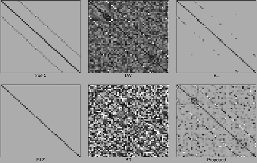
Table 3. Performance comparison in Scenario 3 (Loose Banded Structure). Averages of measures from 200 replicates are listed with parentheses indicating their standard errors.

p	Measure	LW	BL	RLZ	BT	Proposed
30	L1 norm	1.87 (0.02)	1.39 (0.02)	2.19 (0.03)	2.39 (0.01)	1.26 (0.01)
	L2 norm	0.79 (0.00)	0.95 (0.01)	1.06 (0.01)	1.18 (0.00)	0.84 (0.01)
	F norm	2.34 (0.00)	2.47 (0.01)	2.73 (0.01)	2.92 (0.01)	2.12 (0.01)
	ΔEN	4.84 (0.03)	–	5.61 (0.07)	9.41 (0.07)	3.04 (0.03)
	ΔCN	2.97 (0.03)	–	16.16 (0.45)	39.37 (0.97)	1.18 (0.04)
50	L1 norm	2.22 (0.02)	1.57 (0.03)	1.28 (0.01)	3.30 (0.01)	1.35 (0.01)
	L2 norm	0.81 (0.00)	1.06 (0.01)	0.96 (0.01)	1.39 (0.00)	0.89 (0.00)
	F norm	3.20 (0.00)	3.41 (0.01)	3.81 (0.00)	4.50 (0.01)	2.88 (0.01)
	ΔEN	9.71 (0.04)	–	14.00 (0.05)	33.01 (0.10)	5.93 (0.04)
	ΔCN	3.24 (0.02)	–	3.09 (0.16)	172.24 (1.07)	1.22 (0.04)
100	L1 norm	2.74 (0.02)	1.74 (0.03)	1.32 (0.01)	5.58 (0.03)	1.47 (0.01)
	L2 norm	0.82 (0.00)	1.16 (0.01)	0.99 (0.00)	1.60 (0.00)	0.93 (0.00)
	F norm	4.79 (0.00)	5.12 (0.01)	5.41 (0.00)	8.11 (0.00)	4.34 (0.01)
	ΔEN	22.40 (0.05)	–	28.55 (0.07)	177.16 (0.05)	14.38 (0.07)
	ΔCN	3.46 (0.01)	–	2.70 (0.03)	188.17 (1.61)	1.42 (0.03)

Tables 4 and 5 report the comparison results for Scenarios 4 and 5. Compared with Scenario 4 that considers the block diagonal structure, Scenario 5 allows non-zero entries to scatter over the whole covariance matrix. Overall, our proposed method performs better than the LW and BT estimates, and is comparable to the BL and RLZ estimates. Because of the high correlations among the first 20% variables, the BL estimate outperforms the other estimates in terms of the L₁, L₂ and F norm measures. However, the BL method does not guarantee the positive definiteness of the estimate. The performance of the RLZ estimate is reasonably well in Scenario 4, but in terms of the entropy loss and Δ_CN, it is not as good as our proposed estimate. When there is no banded structure such as in Scenario 5, our proposed estimate performs much better than the RLZ estimate.

Table 4. Performance comparison in Scenario 4 (Block Diagonal Structure). Averages of measures from 200 replicates are listed with parentheses indicating their standard errors.

p	Measure	LW	BL	RLZ	BT	Proposed
30	L1 norm	3.71 (0.03)	1.29 (0.04)	1.95 (0.03)	3.33 (0.04)	2.54 (0.05)
	L2 norm	2.40 (0.04)	0.99 (0.04)	1.19 (0.03)	1.92 (0.04)	2.04 (0.05)
	F norm	3.19 (0.02)	1.48 (0.03)	2.49 (0.02)	3.23 (0.03)	2.52 (0.04)
	ΔEN	6.45 (0.04)	–	3.59 (0.03)	10.15 (0.06)	1.99 (0.03)
	ΔCN	18.30 (0.21)	–	27.42 (1.04)	105.25 (3.43)	11.37 (0.17)
50	L1 norm	6.32 (0.04)	2.30 (0.08)	3.27 (0.05)	4.93 (0.08)	4.53 (0.08)
	L2 norm	4.02 (0.07)	1.65 (0.07)	1.85 (0.06)	2.80 (0.07)	3.58 (0.08)
	F norm	5.35 (0.04)	2.26 (0.06)	4.10 (0.03)	4.81 (0.05)	4.21 (0.08)
	ΔEN	12.85 (0.04)	–	10.36 (0.05)	33.05 (0.12)	4.28 (0.06)
	ΔCN	29.13 (0.39)	–	104.90 (3.20)	566.19 (7.55)	18.70 (0.27)
100	L1 norm	12.98 (0.09)	5.00 (0.17)	6.32 (0.11)	9.78 (0.18)	9.78 (0.15)
	L2 norm	8.16 (0.15)	3.25 (0.14)	3.40 (0.13)	5.64 (0.16)	7.43 (0.15)
	F norm	10.81 (0.07)	4.13 (0.13)	7.78 (0.07)	9.07 (0.12)	8.50 (0.15)
	ΔEN	34.30 (0.19)	–	47.04 (0.12)	170.12 (0.27)	15.02 (0.37)
	ΔCN	56.94 (0.83)	–	2347.73 (76.61)	1107.35 (16.41)	30.14 (0.48)

Table 5. Performance comparison in Scenario 5 (Permuted Block Diagonal Structure). Averages of measures from 200 replicates are listed with parentheses indicating their standard errors.

p	Measure	LW	BL	RLZ	BT	Proposed
30	L1 norm	3.64 (0.03)	1.29 (0.05)	4.77 (0.04)	3.24 (0.04)	2.41 (0.05)
	L2 norm	2.29 (0.04)	0.98 (0.04)	2.31 (0.05)	1.86 (0.04)	1.92 (0.05)
	F norm	3.15 (0.02)	1.47 (0.03)	4.24 (0.02)	3.19 (0.03)	2.41 (0.04)
	ΔEN	6.39 (0.04)	–	12.84 (0.16)	10.13 (0.06)	1.95 (0.03)
	ΔCN	17.90 (0.21)	–	126.81 (4.57)	100.51 (2.96)	11.14 (0.16)
50	L1 norm	6.31 (0.05)	2.33 (0.08)	8.18 (0.05)	4.84 (0.08)	4.41 (0.09)
	L2 norm	3.95 (0.07)	1.67 (0.07)	3.63 (0.07)	2.77 (0.07)	3.47 (0.08)
	F norm	5.33 (0.03)	2.27 (0.06)	7.07 (0.03)	4.78 (0.05)	4.12 (0.08)
	ΔEN	12.85 (0.04)	–	48.34 (0.37)	32.91 (0.12)	4.27 (0.06)
	ΔCN	28.64 (0.41)	–	–	565.31 (7.23)	18.37 (0.26)
100	L1 norm	12.97 (0.09)	4.94 (0.16)	15.70 (0.07)	9.90 (0.17)	9.85 (0.15)
	L2 norm	8.21 (0.14)	3.16 (0.13)	9.79 (0.09)	5.71 (0.15)	7.49 (0.14)
	F norm	10.83 (0.07)	4.05 (0.12)	15.01 (0.02)	9.13 (0.11)	8.58 (0.14)
	ΔEN	34.17 (0.19)	–	232.09(1.62)	170.30 (0.28)	15.52 (0.37)
	ΔCN	57.44 (0.78)	–	–	1104.45 (15.87)	30.07 (0.46)

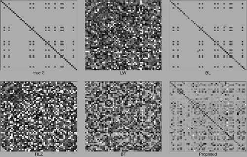
We also present heat maps for one simulated replicate in Figure 2 to elaborate the results in Table 5. The BL estimate has the clearest appearance, where only a few truly zero entries are not identified. However, the estimate is not positive definite, which can be partially caused by these disparities. The LW and RLZ estimates do not capture the structure of the covariance matrix, resulting in less accurate estimation as shown in Table 5. Both the BT estimate and our proposed estimate appear to be capable in restoring the covariance structure in Scenario 5. And our proposed estimate appears to be more stable than BT estimate in terms of CN values reported in Table 5.

Figure 2. Heat maps of the true covariance matrix and various estimates from one replicate of simulations in Scenario 5. Absolute values of entries are used to replace original entries. An entry of magnitude 1 or over is represented by a black square and an entry of magnitude 0 is represented by a white square.

Simulation for Scenario 6 considers the situation where is dense, that is, most entries of are non-zeros. The comparison results of five estimates are shown in Table 6. Overall, our proposed estimate gives better performance than the BL and RLZ estimates. The LW estimate has comparable L₁, L₂ and F norm measures with our proposed estimate, while its entropy loss is larger than that from our proposed estimate. The performance of the BT estimate and our proposed estimate is similar since both of them rely on regularisation. In terms of Δ_CN, our proposed estimate has smaller Δ_CN losses for situations of p = 30 and p = 50. There is no clear ranking among different estimates for p = 100.

Table 6. Performance comparison in Scenario 6 (Dense Structure). Averages of measures from 200 replicates are listed with parentheses indicating their standard errors.

p	Measure	LW	BL	RLZ	BT	Proposed
30	L1 norm	5.77 (0.04)	8.02 (0.06)	7.05 (0.05)	6.12 (0.04)	6.29 (0.04)
	L2 norm	2.41 (0.02)	3.25 (0.03)	2.74 (0.02)	2.70 (0.02)	2.75 (0.02)
	F norm	5.08 (0.02)	6.81 (0.03)	6.32 (0.02)	5.58 (0.02)	5.70 (0.02)
	ΔEN	17.59 (0.11)	–	14.02 (0.21)	11.06 (0.06)	9.26 (0.07)
	ΔCN	50.47 (0.08)	–	80.48 (4.13)	151.05 (4.82)	22.40 (1.66)
50	L1 norm	11.23 (0.04)	14.94 (0.09)	14.14 (0.07)	12.13 (0.06)	12.16 (0.05)
	L2 norm	3.89 (0.02)	4.68 (0.03)	4.34 (0.02)	4.31 (0.02)	4.50 (0.02)
	F norm	9.84 (0.02)	13.41 (0.02)	12.48 (0.02)	10.98 (0.02)	11.13 (0.02)
	ΔEN	100.69 (0.44)	–	69.45 (1.72)	34.05 (0.09)	35.40 (0.42)
	ΔCN	230.50 (0.07)	–	400.15 (33.69)	487.07 (5.03)	143.84 (9.61)
100	L1 norm	29.17 (0.10)	44.62 (0.33)	32.92 (0.04)	34.24 (0.19)	30.88 (0.09)
	L2 norm	7.89 (0.02)	9.87 (0.07)	8.69 (0.01)	9.00 (0.03)	9.04 (0.02)
	F norm	25.78 (0.03)	35.92 (0.08)	30.72 (0.01)	29.91 (0.03)	29.24 (0.03)
	ΔEN	1772.92 (4.55)	–	1825.68 (5.47)	184.01 (0.67)	683.70 (20)
	ΔCN	2831.34 (0.05)	–	2828.37 (0.12)	1371.17 (8.89)	2498.90 (36.92)

To sum up, our proposed estimate outperforms the LW estimate, the BL estimate and the BT estimate in various covariance matrix structures used in the simulation studies. The RLZ estimate gives good performance only when the underlying covariance matrix is banded since it is specially designated for this case. Our proposed estimate is applicable in more general situations where the true covariance matrix is not limited to the banded structure.

5. Real data analysis

To further explore the performance of our proposed covariance matrix estimate, we applied our proposed covariance matrix to a real data analysis. The study is on a stock market data-set. The estimated covariance matrix was used in the equity portfolio allocation.

The common portfolio strategy (Markowitz, 1952) attempts to minimise the risk for a given level of expected return through diversifying the investments in various assets. The risk is generally measured by the variance of the portfolio returns. Denote by the proportions of various assets in the portfolio, and let be the volatility matrix of returns in the asset pool. An optimal portfolio with no-short-sale constraint would be constructed by solving the following quadratic optimisation: (12) where is a vector with entries equal to 1. We expect that an accurate estimate of would lead to a better portfolio strategy. Traditionally, the sample covariance matrix is used to estimate above. However, in many cases, the length of the asset return series used is not big enough compared to the number of assets considered. As pointed out by Michaud (1989), since the objective function involves the covariance matrix, an ill-conditioned matrix estimation may result in unstable solutions of in Equation (12(12) ) and greatly amplifies the error of portfolio allocation. Therefore, the estimate for has to be positive definite such that the quadratic programming of Equation (12(12) ) would not be ill-defined. Moreover, the assets do not have a natural order among them. Based on these conditions, we only include methods producing positive definite and order-invariant estimates in comparison, which are the LW estimate, the BT estimate and our proposed estimate.

We considered the stock return data from companies in the Standard & Poor's 100 index. Because of financial crisis in 2008, we decided to focus on a time zone before 2008. Specifically, we used the weekly return data in 2006 as the training set to build portfolio strategy, and the weekly return data in 2007 to test the performance. Since Mastercard, Visa and Philip Morris International are not listed throughout this time zone, these companies are excluded from the equity pool, and only the remaining 97 stocks are used.

With weekly return data of these 97 stocks in 2006, we built portfolios 1, 2 and 3, using the LW estimate, the BT estimate and our proposed estimate, respectively. Table 7 summarises the averages and the standard deviations of the realised weekly returns for these three portfolios using testing set in 2007. The annual returns from combining 52 weeks’ returns are also included. The results show that portfolio 3 derived from our proposed estimate is better than the other two portfolios with a larger realised weekly return and smaller corresponding standard deviation. Consequently, portfolio 3 provides the highest annual return. It appears that our proposed estimate results in an improvement of portfolio strategy in terms of more realised returns.

Table 7. Summary of realised returns of portfolios built with different covariance matrix estimates.

	Weekly return
		Standard	Annual
Year 2007 (test set)	Average	deviation	return
Portfolio 1 (w/. LW estimate)	0.21 %	1.56 %	10.62 %
Portfolio 2 (w/. BT estimate)	0.19 %	1.58 %	9.89 %
Portfolio 3 (w/. proposed estimate)	0.26 %	1.50 %	13.58 %

We also investigate whether our proposed estimate is sensitive to the choice of the permutation set in Equation (10(10) ), Specifically, we took 200 different sets of randomly selected permutations to obtain our proposed covariance matrix estimates, and further generated 200 portfolios correspondingly. The behaviours of these 200 portfolios are consistent. The standard deviation of annual returns of these portfolios is 0.50% for 2007 (the test set). This value is very small compared with the realised annual returns. With a moderate size of permutation set, K = 30, the impact of permutation set selection appears to be at a quite acceptable level.

6. Discussion

We propose a model averaging covariance matrix estimate with guaranteed positive definiteness based on the MCD. Unlike the Rothman et al.'s estimate, our proposed method is applicable in a general case, not limited to the estimation of banded covariance matrix. Additionally, our proposed estimate is not sensitive to the order of variables used in the MCD. To achieve this property, we develop our estimate described in Equation (10(10) ) through refining a representative group of individual estimates under random permutations. The averaged covariance matrix estimator produces a more accurate estimator with smaller variance than the estimator obtained using a single order of variables in the MCD of covariance matrix. The choice of permutation set is not essential since the mechanism of random selection achieves representativeness. For instance, in our simulation study, our proposed estimate under refinement groups of size 30 and 100 presented similar performance. In the real data analysis, different selection of permutation sets gave the minimal extent of variabilities for the results. Therefore, the guideline for the size of permutation set is to seek the balance between computation convenience and estimation accuracy. A moderate number, like 30, appears to provide adequate performance in practice. Nevertheless, we also notice that the choice of the number of permutations, K, may depend on the number of variables p. A larger number of permutations may be needed to achieve a stable performance of the proposed estimator as p increases. An interesting topic on how to choose an optimal value of K given the number of variables p is left for further study.

Another interesting topic is the study of the convergence rate of the proposed estimator. A potentially useful idea is first to derive the convergence rate of the estimators of the Cholesky factor matrices and under a given order of variables π_k. Then based on the formula in Equation (9(9) ), one could obtain the convergence rate of , and hence the convergence rate of the proposed estimator in Equation (10(10) ). A rigorous proof is under investigation and will be reported elsewhere.

In this work, our proposed model averaging estimate is obtained from the refinement strategy of taking average of several individual estimates of . The refined estimate is positive definite because each individual estimate is positive definite. Alternatively, other strategies may have similar effects. For example, one may choose to refine Cholesky factor matrices s and s in Equation (4(4) ) from individual estimates. Then, the averages of s and the average of s can be used to form a refined covariance matrix estimate with positive definiteness and parsimonious properties. Research along this line will be reported elsewhere.

Acknowledgments

The authors would like to thank the Editor, the Associate Editor and referees for their insightful comments and suggestions. Deng's research is supported by the National Science of Foundation of China (NSFC-71531004).

Disclosure statement

No potential conflict of interest was reported by the authors.

Additional information

Funding

National Science of Foundation of China [grant number NSFC-71531004]; NNSF.

Notes on contributors

Hao Zheng

Hao Zheng holds a Ph.D. in statistics from University of Wisconsin-Madison. He is now a senior biostatistician at Gilead Sciences, Inc.

Kam-Wah Tsui

Kam-Wah Tsui holds a Ph.D. in statistics from University of British Columbia. He is a full professor in department of statistics at University of Wisconsin-Madison. His research interests include decision theory, survey sampling, statistical inference, and Bayesian methods.

Xiaoning Kang

Xiaoning Kang holds a Ph.D. in statistics from Virginia Tech. He is now an assistant professor at International Business College in Dongbei University of Finance and Economics, China. His research interests include high-dimensional data analysis, large covariance matrix estimation, and statistical methodology with financial applications.

Xinwei Deng

Xinwei Deng holds a Ph.D. in statistics from Georgia Institute of Technology. He is now an associate professor in the department of statistics at Virginia Tech. His research interests include interface between machine learning and experimental design, modeling and analysis of high-dimensional data, covariance matrix estimation, and design and analysis of computer experiments.

Appendix. Special case with λ = 0 in Equation (7(7) ) when n > p

Assume that independent and identically distributed are observed and centred. Denote and assume that is non-singular, i.e., n > p. Denote as the estimated covariance matrix from Equation (8(8) ) with λ = 0 in Equation (7(7) ). Then in spite of any permutation of . Below is the proof.

Proof: Based on the sequential regression for Equation (7(7) ), it is known that ⋮

Therefore, the (s, t) entry of the covariance matrix estimate from the sequential regression process is Meanwhile, and the (s, t) entry of the sample covariance matrix is The last equality holds because of Thus, we can establish the result

References

- Bickel, P., & Levina, E. (2008a). Covariance regularization by thresholding. The Annals of Statistics, 36, 2577–2604.
- Bickel, P., & Levina, E. (2008b). Regularized estimation of large covariance matrices. The Annals of Statistics, 36, 199–227.
- Bien, J., & Tibshirani, R. (2011). Sparse estimation of a covariance matrix. Biometrika, 98, 807–820.
- Burman, P. (1989). A comparative study of ordinary cross-validation, v-fold cross-validation and the repeated learning-testing methods. Biometrika, 76, 503–514.
- Chen, Z., & Leng, C. (2015). Local linear estimation of covariance matrices via Cholesky decomposition. Statistica Sinica, 25, 1249–1263.
- Cochran, W. G. (1977). Sampling techniques. New York, NY: John Wiley & Sons.
- Deng, X., & Tsui, K.-W. (2013). Penalized covariance matrix estimation using a Matrix-Logarithm transformation. Journal of Computational and Graphical Statistics, 22, 494–512.
- Fan, J., Xue, L., & Zou, H. (2016). Multitask quantile regression under the transnormal model. Journal of the American Statistical Association, 111, 1726–1735.
- Friedman, J., Hastie, T., & Tibshirani, R. (2010). Regularization paths for generalized linear models via coordinate descent. Journal of Statistical Software, 33, 1–22.
- Golub, G. H., & Van Loan, C. F. (2012). Matrix computations. Baltimore, MD: The Johns Hopkins University Press.
- Hunter, D. R., & Lange, K. (2000). Quantile regression via an MM algorithm. Journal of Computational and Graphical Statistics, 9, 60–77.
- James, W., & Stein, C. (1961). Estimation with quadratic loss. Proceedings of the Fourth Berkeley Symposium on Mathematical Statistics and Probability, 1, 361–379.
- Johnstone, I. M. (2001). On the distribution of the largest eigenvalue in principal components analysis. The Annals of Statistics, 29, 295–327.
- Kullback, S., & Leibler, R. A. (1951). On information and sufficiency. The Annals of Mathematical Statistics, 22, 79–86.
- Ledoit, O., & Wolf, M. (2004). A well-conditioned estimator for large-dimensional covariance matrices. Journal of Multivariate Analysis, 88, 365–411.
- Levina, E., Rothman, A., & Zhu, J. (2008). Sparse estimation of large covariance matrices via a nested Lasso penalty. The Annals of Applied Statistics, 2, 245–263.
- Liu, H., Wang, L., & Zhao, T. (2013). Sparse covariance matrix estimation with eigenvalue constraints. Journal of Computational and Graphical Statistics, 23, 439–459.
- Markowitz, H. (1952). Portfolio selection. The Journal of Finance, 7, 77–91.
- Michaud, R. O. (1989). The Markowitz optimization enigma: Is ‘optimized’ optimal? Financial Analysts Journal, 45, 31–42.
- Pinheiro, J. C., & Bates, D. M. (1996). Unconstrained parametrizations for variance-covariance matrices. Statistics and Computing, 6, 289–296.
- Pourahmadi, M. (1999). Joint mean-covariance models with applications to longitudinal data: Unconstrained parameterisation. Biometrika, 86, 677–690.
- Rothman, A., Levina, E., & Zhu, J. (2010). A new approach to Cholesky-based covariance regularization in high dimensions. Biometrika, 97, 539–550.
- Trefethen, L. N., & Bau III, D. (1997). Numerical linear algebra. Philadelphia, PA: Society for Industrial and Applied Mathematics.
- Wang, Y., & Daniels, M. (2014). Computationally efficient banding of large covariance matrices for ordered data and connections to banding the inverse Cholesky factor. Journal of multivariate analysis, 130, 21–26.
- Xue, L., Ma, S., & Zou, H. (2012). Positive definite l1 penalized estimation of large covariance matrices. Journal of the American Statistical Association, 107, 1480–1491.
Appendix. Special case with λ = 0 in Equation (Equation7(7) ) when n > p