An adaptive lack of fit test for big data

abstract

New technological advancements combined with powerful computer hardware and high-speed network make big data available. The massive sample size of big data introduces unique computational challenges on scalability and storage of statistical methods. In this paper, we focus on the lack of fit test of parametric regression models under the framework of big data. We develop a computationally feasible testing approach via integrating the divide-and-conquer algorithm into a powerful nonparametric test statistic. Our theory results show that under mild conditions, the asymptotic null distribution of the proposed test is standard normal. Furthermore, the proposed test benefits from the use of data-driven bandwidth procedure and thus possesses certain adaptive property. Simulation studies show that the proposed method has satisfactory performances, and it is illustrated with an analysis of an airline data.

Keywords:

• Adaptive test
• asymptotic distribution
• divide-and-conquer algorithm
• massive dataset
• model specification test

1. Introduction

The advancement and prevalence of computer technology in nearly every realm of science and daily life have enabled the collection of ‘big data’. While access to such wealth of information opens the door towards new discoveries, it also poses challenges to the current statistical and computational theory and methodology. Since it is usually computationally infeasible to make inference directly for big data due to the limitation of computing power and memory space, checking model misspecifications is not an easy task.

We shall now present one motivating example. There is an airline on-time data which consists of flight arrival and departure details for all commercial flights from October 1987 to April 2008 in USA. There are 123,534,969 records and 29 variables. And it occupies 11.2GB space. Due to the highly developed transportation system of airplanes, flight delay problem has become more and more serious. An appropriate model is critical for predicting the delay probability of a flight. Suppose that a parametric model is provided according to historical experience. Naturally, before fitting the new data with the proposed model, we want to make sure whether the proposed model is appropriate or not. However, for such big data, many existing softwares have failed to handle it. Since the ‘big data’ problem is not only the size of the data but also the analysis of it takes a significant amount of time and computer memory. Moreover, since the samples in big datasets are typically aggregated from multiple sources (Fan, Han, & Liu, 2014), a computationally feasible and efficient lack-of-fit test is highly desirable for massive datasets.

Let (Y, X) be a random variable in . We have observations (y_i, x_i)^N_{i = 1} from the underlying model E(Y|X = x) = m(x). In a parametric regression model, m(x) is assumed to belong to a parametric family of known real functions on , where . We want to test the null hypothesis that the parametric model is correct for a dataset, say against the alternative hypothesis

A number of nonparametric smoothing-based lack-of-fit tests for small and moderate sample sizes have been proposed during the last 20 years (see González-Manteiga and Crujeiras (2013) for an overview). Among them, some kernel-based tests, such as Zheng (1996) and Hardle and Mammen (1993), are easy to implement when N is not too large. However, the quadratic time complexity and large memory greatly hamper their availability to massive data applications. The main emphasis of this paper is to overcome computational barriers of traditional tests for massive data by using divide-and-conquer (DC) algorithm.

When the data is too large to access the whole dataset once in a processor, one strategy is to divide and conquer. A DC algorithm works by recursively breaking down a big dataset into two or more subsets which are manageable and then analyse these subsets separately and combine the sub-solutions as the final one. Recently, DC strategy has been widely used in analysing massive data concerning parameters estimation of parametric regression (Battey, Fan, Liu, Lu, & Zhu, 2015; Chen & Xie, 2014; Lin & Xi, 2011; Schifano, Wu, Wang, Yan, & Chen, 2016), nonparametric regression curve estimation (Cheng & Shang, 2015; Zhang, John, & Martin, 2013; Zhao, Cheng, & Liu, 2016) and bootstrap issue (Kleiner, Talwalkar, Sarkar, & Jordan, 2015). However, little attention has been paid to the lack-of-fit test of parametric regression models for massive data. We combine the DC method with the test statistic proposed by Zheng (1996) to solve the computational problem. We separate the data into K subsets evenly with each subset having the same sample size, n. Building test statistic based on each subsample and then averaging these test statistics to obtain the final one, the computational complexity of the test statistic is reduced from N² to O(Kn²) and the calculation occupies much less memory, which is quite useful for big data.

The choice of smoothing parameter inherent in smoothing-based test plays an essential role, which refers to bandwidth parameter in kernel-based tests. As criteria used for smoothing parameter selection in nonparametric estimation differ from testing, it is inappropriate to apply prevalent smoothing parameter selection approaches for nonparametric estimation in the context of nonparametric hypothesis testing. There has been a growing amount of literatures on smoothing parameter selection in testing (e.g., Eubank, Ching-Shang, & Wang, 2005; Gao & Gijbels, 2008; Guerre & Lavergne, 2005; Hart, 1997; Horowitz & Spokoiny, 2001; Kulasekera & Wang, 1997; Ledwina, 1993; Zhang, 2003a, 2003b). A popular approach is to combine the test statistics obtained from using a series of suitable bandwidth values (Guerre & Lavergne, 2005; Horowitz & Spokoiny, 2001; Zhang, 2003a), resulting in an adaptive test. For instance, Horowitz and Spokoiny (2001)'s test is a maximum test with respect to a set of bandwidth values. They obtained critical values of their test statistic by bootstrap, and thus it is rather time-consuming for big datasets. We suggest to combine the method in Horowitz and Spokoiny (2001) with the DC method to construct an adaptive and computationally feasible nonparametric lack-of-fit test.

The paper is organised as follows. Section 2 describes the test statistics and bandwidth selection procedure. Asymptotic properties are discussed. Simulation studies and a real data analysis are given in Section 3. Section 4 contains some concluding remarks. Technical proofs are provided in the Appendix.

2. Methodology

The nonparametric test proposed by Zheng (1996) combines the kernel method and the conditional moment test. The key idea is to use a kernel-based sample estimator of the conditional moment E{E²(ϑ_i|x_i)f(x_i)}, where and f(·) is the density function of x_i. The test statistic based on the whole sample is where is a p-dimensional kernel function and , h_N is the bandwidth depending on N. , where is an estimator of . Denote the corresponding test based on Z_N as ZH test. Clearly, Z_N is a computation-intensive when N is large, limiting its usefulness for massive data.

We use the DC strategy to solve the problem by separating the data into K subsets evenly and make each subset have the same sample size n. Denote the test statistic based on the kth subset of data as V_k, where h_n is the bandwidth based on the dataset of size n. , where is a DC-based estimator of (Lin & Xi, 2011). The asymptotic null mean and variance of nh^p/2_nV_k are 0 and δ² according to Zheng (1996) as h_n → 0 and nh^p_n → ∞, where A consistent estimator of δ² using the kth subset data is

Since this test is sensitive to the bandwidth selection, a robust test is desired. Following the selection approach proposed in Horowitz and Spokoiny (2001) and Zhang (2003a), for each normalised V_k, we take the maximum of the normalised statistic with respect to a candidate set of h_n which is defined as . The maximum and minimum elements in are denoted as h_max and h_min, respectively. Suppose there are m elements in and m is finite. This procedure is intended to reduce the dependency of the proposed test on individual h. It makes the test suitable for a broader class of alternatives compared with the original test depending on one h, leading to an adaptive test. Our final test statistic based on K subsets data is For the sake of simplifying notations, we denote as D_k(h) and the test based on D_N as DM test. {max _{1 ⩽ s ⩽ m}D_k(h_s)}^K_{k = 1} can be treated as K independent identically distributed random variables. On the basis of the above discussion and some mild conditions, we can establish the limiting behaviour of D_N. The following are some assumptions needed in our theories.

Assumption 2.1:

The density function f(x) of X is bounded away from 0 and has bounded first-order derivatives.

Assumption 2.2:

g( ·, ·) is uniformly bounded in x and and is twice continuously differentiable with respect to , with first- and second-order derivatives uniformly bounded in x and .

Assumption 2.3:

is a bounded and symmetric density function.

Assumption 2.4:

The random variables ϵ_i are independent with E(ϵ_i|x_i) = 0. We assume that σ²(x_i), E(ϵ⁴_i|x_i) = σ⁴(x_i) are uniformly bounded in i and have uniformly bounded first-order derivatives for all i.

Assumption 2.5:

Let for any m(·). For any m(·), is unique and is the estimator of such that . Under H₀, .

The first theorem is similar to Theorem 1 in Zhang (2003a). For notational convenience, we write the index as max _{1 ⩽ s ⩽ m}D_k(h_s).

Theorem 2.1:

Suppose Assumptions 2.1–2.5 hold. Under the null hypothesis, for a finite integer m ≥ 1, as h_max → 0, nh^p_min → ∞, we have where (U₁,… , U_m)^T is a mean-zero normal random vector with a covariance matrix Γ = (γ_st)_1≤s,t≤m, with γ_st = γ_ts = δ²_st/δ², and l_st = h_s/h_t for 1 ≤ s, t ≤ m.

δ² can be consistently estimated by and δ²_st can be consistently estimated by ,

The mean of max _{1 ⩽ s ⩽ m}U_s can be obtained by Afonja (1972). Then, we use it to approximate the mean of max _{1 ⩽ s ⩽ m}D_k(h_s) based on Theorem 2.1 and DasGupta (2008, Theorem 6.2). Therefore, the asymptotic null distribution of D_N can be easily got through Lindeberg--Levy central limit theorem and Slutsky's theorem.

Theorem 2.2 (Null hypothesis):

Given Assumptions 1–5, under H₀, as K → ∞, nh^p → ∞, h → 0, we have that with where R_st = {r_s,vw,t}, r_s,vw,t is the partial correlation between (U_s − U_v) and (U_s − U_w) given (U_s − U_t). Φ(x) denotes the cumulative distribution functions of the standard normal distribution. s² is the sample variance computed on {max _{1 ⩽ s ⩽ m}D_k(h_s)}^K_{k = 1}.

Theorem 2.2 reveals that the asymptotic null distribution of our test is normal under some mild conditions. Based on this theorem, we can calculate the critical value for our test. Another appealing result is that the convergence rate of D_N is K^−1/2 which can be faster than the nonparametric convergence rate (Nh^p/2_N)^{− 1} of ZH test provided that K is large enough. The proposed test can detect against a broad class of alternatives via the above bandwidth selection procedure, and hence it is an adaptive test. And it can also accelerate the calculation of ZH test and effectively reduce the demand for memory.

For the convenience of the presentation of the next result, we denote the variance of max _{1 ⩽ s ⩽ m}D_k(h_s) under the null hypothesis as ν². The next result considers the asymptotic behaviour of D_N under the local alternative m(x) = g(x; θ*) + K^{− 1/4}l(x).

Theorem 2.3 (Local alternative):

Suppose Assumptions 1–5 hold. Assume K → ∞, nh^p → ∞, h → 0, under the local alternative,

Theorem 2.3 guarantees that the D_N test has nontrivial power against contiguous alternative of order K^−1/4. Together with Theorem 2.2, Theorem 2.3 reveals that the D_N cannot distinguish alternatives of order smaller than K^−1/4 from the null.

3. Numerical analysis

3.1. Simulation studies

In this section, we conduct a sample simulation to check the finite samples performance of the proposed DM test based on the size and power. We aim to show the advantages of our test from three perspectives which are computability, time saving and adaptiveness in terms of massive data. And the comparisons are made between ZH test, DM test and GL test, where GL test is an adaptive and asymptotic normal test proposed by Guerre and Lavergne (2005). The data is generated as in Zheng (1996). z₁ and z₂ are generated from the standard normal distribution. The regressors are given by . Two cases of error term ϵ are considered following the standard normal and a standardised Student with five degrees of freedom distribution. The simulation is based on models which are considered in Zheng (1996) and Fan and Li (2000).

Model 0: Y = 1 + X₁ + X₂ + ϵ;

Model 1: Y = 1 + X₁ + X₂ + bX₁X₂ + ϵ, b ∈ [0, 1];

Model 2: Y = 1 + X₁ + X₂ + 2sin (bX₁)sin (bX₂) + ϵ, b ∈ [0, 40].

We treat model 0 as our null hypothesis, which assumes that the real regression model is linear. Model 1 corresponding a fixed alternative is designed to see the power of the test against high-order terms. To investigate the power of the test against a high(low) frequency fixed alternative, we consider model 2. In model 2, small(large) value of b represents low(high) frequency alternative. The kernel function is chosen to be the bivariate standard normal density function We choose m = 3 for multiple bandwidths and set . The bandwidth h is chosen to be c₀n^−1/6 for DM test, where c₀ = 0.25 is a constant in order to control the size of the test. h is set to be 0.25N^−1/6 for ZH and GL test as these test statistics are constructed based on sample size N. Denote h₁ = 0.125N^−1/6, h₂ = 0.25N^−1/6, h₃ = 0.5N^−1/6. The penalty sequence for GL test is chosen as , where c = 1, 1.5, 2. The critical values for the three tests are based on the standard normal. For DM test when m = 3, We approximate μ via estimating δ² and δ²_st by and , respectively.

These three tests are compared under the same time budget as time is an important evaluation criterion for massive data analysis. For DM test, we consider two settings of (N, K), which are (20,000, 40), (40,000, 100). Under the same time budget, we choose corresponding N = 7400, 9500 for ZH test, N = 4800, 6200 for GL test. This illustrates the advantage of our test in time. Under the null hypothesis, each experiment is based on 10,000 replications and 1000 under the alternatives. What we can conclude from Tables 1 and 2 is that both ZH and DM test can control type-I error. For DM test, the approximation is more acceptable when N =40,000, K =100 than N =20,000, K = 40. For GL test, there is another tuning parameter c needed to be chosen. c plays a critical role in the approximation under null hypothesis. According to the simulation results, we set c = 2 in the following power comparison experiments.

Table 1. Empirical size, normal errors.

		DM	GL			ZH
		K	c
N	α	40 (100)	1	1.5	2	h1	h2	h3
	1.00	1.28	6.19	1.64	0.79	0.99	0.81	0.81
20,000 (4800, 7400)	5.00	6.08	9.77	5.30	4.55	4.68	4.82	4.49
	10.00	11.10	14.31	10.14	9.44	9.72	9.88	9.14
	1.00	1.23	6.22	1.52	0.72	0.97	0.99	0.63
40,000 (6200, 9500)	5.00	5.57	9.77	5.08	4.37	4.80	5.04	4.55
	10.00	10.69	14.37	9.96	9.35	10.11	9.91	9.33

Percentages of rejection at 1%, 5%, 10% nominal levels.

Table 2. Empirical size, Student errors.

		DM	GL			ZH
		K	c
N	α	40 (100)	1	1.5	2	h1	h2	h3
	1.00	1.54	6.55	1.68	0.83	0.99	1.04	0.97
20,000 (4800, 7400)	5.00	5.65	9.81	4.87	4.07	5.09	5.27	4.45
	10.00	10.95	14.66	9.97	9.27	10.36	10.38	9.35
	1.00	1.00	6.65	1.65	0.83	0.96	0.89	0.85
40,000 (6200, 9500)	5.00	5.01	10.10	5.30	4.59	4.75	4.61	4.17
	10.00	9.54	14.93	10.38	9.72	9.61	9.06	9.11

Percentages of rejection at 1%, 5%, 10% nominal levels.

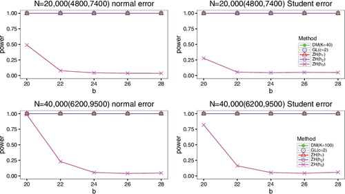
The simulation reveals that the performance of ZH test for different models varies with h. ZH(h₃) behaves the best under Model 1 and low frequency of Model 2. But it has poor performance for high-frequency model. However, ZH(h₁) leads to the opposite results. ZH(h₂) is the most robust. It has good performance for both of the proposed alternative models. It is difficult to find out this robust h in practical applications, while our test is capable of robustness. Figures 1 and 2 show that DM test has power closer to GL test, and ZH(h₂) for model 1 and low-frequency case of model 2. Figure 3 explains that DM test has power closer to the best case of ZH test, which is obtained via the smaller h₁ under high-frequency case of model 2. DM test displays the same adaptive property as GL test. However, it requires less memory than GL test and ZH test under the same time budget. GL test and ZH test are either time-consuming or memory hungry which hinder the scalability to massive datasets.

Figure 1. Comparison of power curves under model 1 of two different error terms at significant level α = 0.05. We set (N, K) = (20,000, 40), (40,000, 100) for DM test. N = 4800, 6200 for GL test. N = 7400, 9500 for ZH test.

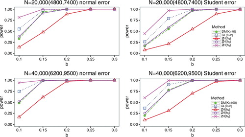
Figure 2. Comparison of power curves under low frequency of model 2 based on two different error terms at significant level α = 0.05.

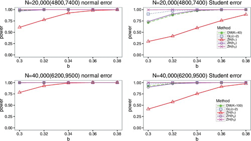
Figure 3. Comparison of power curves under high frequency of model 2 based on two different error terms at significant level α = 0.05.

Moreover, we compare DM test with ZH test based on the whole dataset to study the effect of K on the power performance. K is chosen to be {20, 40, 50} and N = 20, 000. The results under model 1 are reported in Tables 3 and 4. Model 2 follows the same trend and thus is not included. The tables show that the power loss gets more as K gets larger for DM test compared with ZH test.

Table 3. Empirical power of DM test and ZH test based on the whole dataset when the error distribution is normal.

	DM			ZH
	K			h
b	20	40	50	h1	h2	h3
0.1	46.1	32.8	26.8	52.1	95.1	100
0.15	99.4	94.0	89.3	98.9	100	100
0.2	100	100	100	100	100	100
0.25	100	100	100	100	100	100
0.3	100	100	100	100	100	100

Percentages of rejection at 5% nominal levels.

Table 4. Empirical power of DM test and ZH test based on the whole dataset when the error distribution is Student.

	DM			ZH
	K			h
b	20	40	50	h1	h2	h3
0.1	20.7	16.1	13.1	22.6	59.9	96.1
0.15	72.9	55.0	47.0	70.4	100	100
0.2	99.5	96.1	93.7	100	100	100
0.25	100	100	99.9	100	100	100
0.3	100	100	100	100	100	100

Percentages of rejection at 5% nominal levels.

3.2. Real data analysis

In this section, we will revisit the airline on-time data for illustrating the proposed test. A flight is considered delayed when it arrived 15 or more minutes later than the schedule. Many researchers use logistic regression to model the probability of late arrival (binary; 1 if late by more than 15 minutes, 0 otherwise; denote as y) as a function of variables may lead to flight delay. We use the logistic regression model to investigate the relationship of scheduled departure time (continuous, x₁), scheduled arrival time (continuous, x₂), distance (continuous, in thousands of miles, x₃) with late arrival. Since GL and ZH tests cannot handle such big data, only the proposed test is implemented to check the goodness of fit of this model. We get N = 120, 748, 239 observations after removing the missing values. K is chosen to be 10,000. The bandwidth set is The p-value of the proposed test is estimated as 0 which indicates that this model is inadequate to illustrate the late arrival probability. This does not come as a surprise to us, because the weather conditions and mechanical problems are also the causes of flight delay which are not included in the model.

4. Concluding remarks

In this article, we give a test aim to solve the scalability of the traditional nonparametric smoothing-based lack-of-fit test to massive datasets. We focus on two issues which are computability and smoothing parameter selection. The proposed test combines the DC procedure and a simple bandwidth selection method. Theoretically, our test has a manageable asymptotic null distribution. Under the null hypothesis, we use the mean of max _{1 ⩽ s ⩽ m}U_s to approximate max _{1 ⩽ s ⩽ m}D_k(h_s)'s mean in each subset, where (U₁,… , U_m)^T is a multivariate normal distribution. To ensure the accuracy of approximation, we need to make sure that the sample size of each subset is large enough. This condition is easy to achieve for massive data. In addition, our test is advantageous to save computational time and memory space. Simulation studies verified the above theoretical properties as well as the adaptiveness.

Acknowledgments

The authors are grateful to the editor and two anonymous referees for their comments that have greatly improved this paper.

Disclosure statement

No potential conflict of interest was reported by the authors.

Additional information

Funding

This paper was supported by the National Natural Science Foundation of China [grant number 11431006], [grant number 11690015], [grant number 11371202], [grant number 11622104].

Notes on contributors

Yanyan Zhao

Yanyan Zhao is a Ph.D. candidate at the Institute of Statistics, Nankai University, Tianjin, China.

Changliang Zou

Changliang Zou is a professor at the Institute of Statistics, Nankai University, Tianjin, China.

Zhaojun Wang

Zhaojun Wang is the corresponding author and professor at the Institute of Statistics, Nankai University, Tianjin, China.

Appendix

In the proofs, without loss of generality, we assume q = 1.

Lemma A.1:

Given Assumptions 2.1–2.5. Under the null hypothesis, as .

Proof:

Similar to the proof of Lemma 3.3e of Zheng (1996), we can easily get the result of the first part. The second part is as follows:

S_n is a standard U-statistic with We just need to show that E(‖H_n‖²) = o(n), Therefore, by Lemma 3.1 of Powell, Stock, and Stoker (1989), we have proved the conclusion.

Proof of Theorem 2.1

Proof:

Under the null hypothesis, as so we denote V_k = V_1k − 2V_2k + V_3k, where Then,

Since based on Lemma A.1, we denote D*(h_s) = nh^p/2_sV_1kδ^{− 1}. We just need to show

(a)	, where Γ = (γst)1 ≤ s, t ≤ m;
(b)	; .

Then, the main results of Theorem 2.1 can be obtained directly via Slutsky's theorem and Continuous Mapping theorem.

(a)

Choose m = 2 as an illustration, for every , we have c1hp/21V1k(h1) + c2hp/22V1k(h2) is a U-statistic with kernel Hn = Hn1 + Hn2, where , . By checking the conditions in Theorem 1 of Hall (1984) via the same way with Zheng (1996), we have So there is a , where (U1, U2)T ∼ N2(0, Γ) such that for every . By Cramer–Wold device, we have . Next, we determine the entries of covariance matrix Γ. Denote (x1 − x2)/h1 = u, l12 = h1/h2, we have and Then, EH2n = EH2n1 + EH2n2 + 2EHn1Hn2 = c21δ2/2 + c22δ2/2 + c1c2δ12 + o(1). So, Obviously, Then, we obtain that Similar result can be derived for m > 2 with lst = hs/ht, So, by continuous mapping theorem, we have

(b)

Since m is finite, from Lemma 3.3d in Zheng (1996) and Bonferroni inequality, we have the results of (b).

Proof of Theorem 2.2

Proof:

Since As , then the results of Theorem 2.2 follows .

We elucidate the proof based on Lindeberg--Levy central limit theorem. First, we approximate the mean by asymptotic. Afonja (1972) presents a method for finding the mean of maximum of correlated normal variates. By using their Corollary 2, we can get the mean of is with and r_{s, v; w, t} is the partial correlation between (U_s − U_v) and (U_s − U_w) given (U_s − U_t). Φ(x) denotes the cumulative distribution functions of the standard normal distribution.

For s² is a consistent estimator of variance of , the theorem results directly follows Lindeberg--Levy central limit theorem and Slutsky's theorem as K → ∞.

Proof of Theorem 2.3

Proof:

Under the local alternative, denote

We proceed with a decomposition of

Through tedious calculation we have, under local alternative, and As nh^p → ∞, h → 0, we have . Together with Theorem 2.2, we can get the results of Theorem 2.3.

References

- Afonja, B. (1972). The moments of the maximum of correlated normal and t-variates. Journal of the Royal Statistical Society B, 34, 251–262.
- Battey, H., Fan, J., Liu, H., Lu, J., & Zhu, Z. (2015). Distributed estimation and inference with statistical guarantees. arXiv:150905457.
- Chen, X., & Xie, M. (2014). A split-and-conquer approach for analysis of extraordinarily large data. Statistica Sinica, 24, 1655–1684.
- Cheng, G., & Shang, Z. (2015). Computational limits of divide-and-conquer method. arXiv:151209226.
- DasGupta, A. (2008). Asymptotic theory of statistics and probability (1st ed. ). New York, NY: Springer.
- Eubank, R. L., Ching-Shang, L., & Wang, S. (2005). Testing lack of fit of parametric regression models using nonparametric regression techniques. Statistica Sinica, 15, 135–152.
- Fan, Y., & Li, Q. (2000). Consistent model specification tests: Kernel-based tests versus Bierens’ ICM tests. Econometric Theory, 16, 1016–1041.
- Fan, J., Han, F., & Liu, H. (2014). Challenges of big data analysis. National science review, 1(2), 293–314.
- Gao, J., & Gijbels, I. (2008). Bandwidth selection in nonparametric kernel testing. Journal of the American Statistical Association, 484, 1584–1594.
- González-Manteiga, W., & Crujeiras, R. (2013). An updated review of goodness-of-fit tests for regression models. Test, 22, 361–411.
- Guerre, E., & Lavergne, P. (2005). Data-driven rate-optimal specification testing in regression models. Annals of Statistics, 33, 840–870.
- Hall, P. (1984). Central limit theorem for integrated square error of multivariate nonparametric density estimators. Journal of Multivariate Analysis, 14, 1–16.
- Hardle, W., & Mammen, E. (1993). Comparing nonparametric versus parametric regression fits. Annals of Statistics, 21, 1926–1947.
- Hart, J. (1997). Nonparametric smoothing and lack-of-fit tests (1st ed. ). New York, NY: Springer.
- Horowitz, J., & Spokoiny, V. (2001). An adaptive, rate-optimal test of parametric mean-regression model against a nonparametric alternative. Econometrica, 69, 599–631.
- Kleiner, A., Talwalkar, A., Sarkar, P., & Jordan, M. I. (2015). A scalable bootstrap for massive data. Journal of the Royal Statistical Society: Series B, 76(4), 795–816.
- Kulasekera, K., & Wang, J. (1997). Smoothing parameter selection for power optimality in testing of regression curves. Journal of the American Statistical Association, 438, 500–511.
- Ledwina, T. (1993). Data-driven version of Neymans smooth test of fit. Journal of the American Statistical Association, 89, 1000–1005.
- Lin, N., & Xi, R. (2011). Aggregated estimating equation estimation. Statistics and Its Inference, 4, 73–83.
- Powell, J., Stock, J., & Stoker, T. (1989). Semiparametric estimation of index coefficients. Econometrics, 57, 1403–1430.
- Schifano, E., Wu, J., Wang, C., Yan, J., & Chen, M.-H. (2016). Online updating of statistical inference in the big data setting. Technometrics, 58, 393–403.
- Zhang, C. (2003a). Adaptive tests of regression functions via multiscale generalized likelihood ratios. Canadian Journal of Statistics, 31, 151–171.
- Zhang, C. (2003b). Calibrating the degrees of freedom for automatic data smoothing and affective curve checking. Journal of the American Statistical Association, 98, 609–629.
- Zhang, Y., John, D., & Martin, W. (2013). Divide and conquer kernel ridge regression. Journal of Machine Learning Research WCP, 30, 592–617.
- Zhao, T., Cheng, G., & Liu, H. (2016). A partially linear framework for massive heterogeneous data. Annals of Statistics, 44, 1400–1437.
- Zheng, J. (1996). A consistent test of functional form via nonparametric estimation techniques. Journal of Econometrics, 75, 263–289.