Bayesian analysis of series system with dependent causes of failure

ABSTRACT

Most studies of series system assume the causes of failure are independent, which may not hold in practice. In this paper, dependent causes of failure are considered by using a Marshall–Olkin bivariate Weibull distribution. We derived four reference priors based on several grouping orders. Gibbs sampling combined with the rejection sampling algorithm and Metropolis–Hastings algorithm is developed to obtain the estimates of the unknown parameters. The proposed approach is compared with the maximum-likelihood method via simulation. We find that the root-mean-squared errors of the Bayesian estimates are much smaller for the case of small sample size, and that the coverage probabilities of the Bayesian estimates are much closer to the nominal levels. Finally, a real data-set is analysed for illustration.

Keywords:

• Reference prior
• Bayesian analysis
• Weibull distribution
• Gibbs sampling
• Metropolis–Hastings algorithm

1. Introduction

In reliability and survival analysis, it is quite common that a series system or an individual might fail because of one of several causes of failure (or competing risks). A researcher is interested in a specific cause in the presence of other causes. In the statistical literature, this problem is known as the competing risks model, and the series system is a typical competing risk model. Data for a competing risks model may consist of failure times and other variables indicating the causes of failure, which may be dependent or independent. Most of the literature assumes the causes of failure are independent. See, for example, Kozumi (2004), Kundu, Kannan, and Balakrishnan (2003), Pareek, Kundu, and Kumar (2009), Mazucheli and Achcar (2011), Cramer and Schmiedt (2011), Xu and Tang (2011), Xu, Basu, and Tang (2014) and AL-Hussaini, Abdel-Hamid, and Hashem (2015).

However, the independence assumption among the causes of failure is often unrealistic. For instance, in a tug of war, failure of a player causes additional pressure on the team and poses an increased risk of failure to the remaining members. In other words, a positive dependence between failure times is imposed. Thus, the causes of failure being dependent are more practical. Wang and Ghosh (2003) studied dependent competing risks model with absolutely continuous bivariate exponential lifetime distribution under two non-informative priors (Laplace prior and Jeffreys prior). Lindqvist and Skogsrud (2009) have focused on modelling dependent competing risks in reliability by considering first the passage times of Wiener processes. Dijoux and Gaudoin (2009) proposed an alert-delay model which is a new model of dependent competing risks for maintenance and reliability analysis. Dimitrova, Haberman, and Kaishev (2013) demonstrated how copula functions can be applied in modelling dependence between lifetime random variables in the context of competing risks and studied the impact of removing one or more causes of death on the overall survival. When there is a positive probability of simultaneous failure, the most widely used model is the Marshall–Olkin bivariate lifetime model. The Marshall–Olkin bivariate exponential (MOBE) model, proposed by Marshall and Olkin (1967), has been used extensively to analyse two dependent causes of failure. Guan, Tang, and Xu (2013) considered the objective Bayesian analysis of dependent competing risks model using MOBE distribution. However, the MOBE distribution is very limited, because the hazard function is constant or the marginal function is strictly decreasing. Then the Marshall–Olkin bivariate Weibull (MOBW) distribution which was raised by Marshall and Olkin (1967) can make up this deficiency, and has been long enjoyed popularity in reliability (see Kundu & Dey, 2009; Kundu & Gupta, 2013; and the references therein). Feizjavadian and Hashemi (2015) developed the maximum-likelihood estimators (MLEs) and approximated MLEs of the unknown parameters when the lifetime of the two causes of failure follows MOBW distribution.

In this paper, Bayesian method will be used to analyse dependent competing risks model when the MOBW distribution is assumed. Both subjective Bayesian analysis and objective Bayesian analysis are popular in practice. Subjective Bayesian analysis is based on informative priors, i.e. conjugate prior. In such a case, the prior information is used to specify the hyperparameters in the prior distribution. However, prior distribution is not easy to elicit, especially in complex models. Then objective Bayesian analysis by using non-informative priors is preferred. The three most used non-informative priors are Laplace prior (Laplace, 1812), Jeffreys prior (Jeffreys, 1961) and reference prior (Bernardo, 1979). Laplace prior uses a constant prior distribution for the unknown parameters, which is quite easy to specify. However, it is not invariant under reparameterisation, and usually leads to an improper posterior distribution. Jeffreys prior, which is proportional to the square root of the determinant of the Fisher information matrix, has been proved to be successful in single-parameter problems. However, Jeffreys prior is often seriously deficient in multi-parameter problems. To overcome the deficiencies of the Jeffreys prior, Bernardo (1979) proposed the reference prior which works well in multi-parameter problems. It is invariant under reparameterisation and typically produces proper posteriors. The reference prior is the Jeffreys prior in usual single-parameter problems. This approach is very successful in various practical problems (see Xu & Tang, 2010; Xu, Tang, & Sun, 2015). Thus, we will consider noninformative priors for the unknown parameters in the proposed model. To the best of our knowledge, we are the first to develop Bayesian approach, especially objective Bayesian method, to analyse dependent competing risks model using the MOBW distribution. In particular, the reference priors are formally derived, and the properties of these reference priors are studied.

The paper is organised as follows. In Section 2, we describe the MOBW model. The Fisher information matrices under the original and transformed parameters are presented in Section 3. Section 4 is devoted to derive four reference priors under different grouping orders. In Section 5, the propriety of the posterior distribution under different reference priors are proved, and the Gibbs sampling procedures are given to obtain the Bayesian estimates. In Section 6, a simulation is given for illustration. A real data-set is analysed in Section 7. Finally, some concluding remarks are made in Section 8.

2. Marshall–Olkin bivariate Weibull distribution

The MOBW model can be described as follows. It is assumed that U₀, U₁ and U₂ are three independent random variables, and where ∼ means following in distribution and WE(α, λ) denotes a Weibull distribution with the parameters α > 0 and λ > 0. For a WE(α, λ) distribution, the probability density function (PDF), the cumulative distribution function (CDF) and the survival function (SF) for x > 0 are respectively.

Let X₁ = min {U₀, U₁} and X₂ = min {U₀, U₂}, then (X₁, X₂) has the MOBW distribution with the parameters (α, λ₀, λ₁, λ₂), and it will be denoted as MOBW (α, λ₀, λ₁, λ₂). Thus, the joint SF of MOBW (α, λ₀, λ₁, λ₂) can be written as (2.1) Therefore, the joint PDF of X₁ and X₂ can be written as (2.2) where From the above equations, we note that the MOBW distribution has both an absolute continuous part ( f₁(x₁, x₂) and f₂(x₁, x₂)) and a singular part ( f₀(x)). For more details about the MOBW distribution, we can refer to Bemis, Bain, and Higgins (1972) and Kundu and Dey (2009).

3. Data and Fisher information matrix

3.1. Data and likelihood function

Suppose that a series system (or a disease) has two causes of failure. The lifetime of the jth cause of failure is X_j (j = 1, 2), and (X₁, X₂) ∼ MOBW (α, λ₀, λ₁, λ₂). Then the distribution of the lifetime of the series system T = min (X₁, X₂) is WE(α, λ₀ + λ₁ + λ₂). Assume that there are n series systems in a lifetime experiment. Let (X_1i, X_2i) be the lifetime of the two causes of failure in the ith system. Therefore, the observed data are (T_i, δ_1i, δ_2i), i = 1, 2,… , n, where T_i = min (X_1i, X_2i), δ_1i = I(X_1i < X_2i), δ_2i = I(X_1i > X_2i), I(A) denotes the indicator function of event A. Let λ = λ₀ + λ₁ + λ₂, we can obtain the following facts easily.

Lemma 3.1:

For i = 1,… , n, we have

(1)	X1i ∼ WE(α, λ0 + λ1), X2i ∼ WE(α, λ0 + λ2),
(2)	Ti and (δ1i, δ2i) are independent,
(3)

Denote and given the observed data (T_i, δ_1i, δ_2i), i = 1, 2,… , n, the likelihood function

is (3.1) Then the log-likelihood function can be written as

3.2. Fisher information matrix

The second-order partial derivatives of the log-likelihood function are as follows: where q = 0, 1, 2, ρ = 0, 1, 2, q ≠ ρ. Denote Y_i = λT^α_i, i = 1, 2, …, n, then Y_i follows the exponential distribution with hazard rate 1. For ν ≥ 1, let r_ν = ∫^∞₀(ln y)^νe^{− y}dy, which is the νth moment of ln Y_i. Then, After some algebraic calculations, we get where k(x) = 1 + 2r₁ + r₂ − 2(r₁ + 1)ln x + (ln x)², q = 0, 1, 2, ρ = 0, 1, 2, q ≠ ρ. Thus, the Fisher information matrix of (α, λ₀, λ₁, λ₂) has the following form:

3.3. Reparameterisation

In practice, the engineers may be interested in the hazard rate function of the series system, which is αλt^{α − 1}. λ affects the scale of the hazard rate function, and α will determine whether the hazard rate function is decreasing (0 < α < 1), constant (α = 1) or increasing (α > 1). Thus, we take the following transformation: where θ₂ and θ₃ are the probabilities that the failure of series system is due to the first and second causes of failure, respectively. The transformation from (α, λ₀, λ₁, λ₂) to (α, θ₁, θ₂, θ₃) is one-to-one with the inverse transformation After reparameterisation, the likelihood function (3.1(3.1) ) becomes (3.2) The Jacobian matrix of the transformation is where 0 < θ₁ < ∞, 0 < θ₂ + θ₃ < 1.

Lemma 3.2:

The Fisher information matrix of (α, θ₁, θ₂, θ₃) has the following form:

Due to the practical meanings of (α, θ₁, θ₂, θ₃), all the derivations will be based on the new parameters in the following sections. If one is interested in the original parameters, the proposed method in this paper is also suitable.

4. Reference priors

Berger and Bernardo (1992) developed a general algorithm to derive the reference prior. The algorithm needs to divide the parameters into several groups according to the importance of interest. Jeffreys prior treats all the parameters equally, and is shown to yield a decidedly inferior posterior distribution in multivariate-parameter problems (Yang & Berger, 1994). Sometimes, Jeffreys prior will result in an inconsistent estimator of the parameters. The benefit of grouping the parameters is that the prior can be obtained in terms of inferential importance of parameters, and usually results in a proper posterior distribution. Thus, before deriving the reference priors, we should divide the parameters {α, θ₁, θ₂, θ₃} according to the inferential importance. For example, the notation {α, (θ₁, θ₂, θ₃)} will be used to represent the case that the parameters are divided into two groups, with α being the most important and θ₁, θ₂, θ₃ being of equal importance. Similarly, {α, θ₁, (θ₂, θ₃)} represents that the parameters are separated into three groups, with α being the most important and (θ₂, θ₃) being the least important. Ghosh and Mukerjee (1991) and Berger and Bernardo (1992) suggested that switching the role of the parameters of interest and nuisance parameters sometimes gives a reasonable reference prior. We will consider the grouping orders {(α, θ₁), (θ₂, θ₃)}, {(θ₂, θ₃), (α, θ₁)}, {α, (θ₁, θ₂, θ₃)}, {(θ₂, θ₃), α, θ₁}, {α, θ₁, θ₂, θ₃}, {θ₃, θ₂, θ₁, α}, {θ₁, (α, θ₂, θ₃)}, {(θ₂, θ₃), θ₁, α}.

Theorem 4.1:

The possible grouping ordering reference priors of (α, θ₁, θ₂, θ₃) are listed in Table 1, and

Table 1. Possible reference prior of (α, θ₁, θ₂, θ₃).

Ordered	Reference prior	Reference prior for
grouping	for (α, θ1, θ2, θ3)	(α, λ0, λ1, λ2)
{(α, θ1), (θ2, θ3)}	ω1(α, θ1, θ2, θ3)	π1(α, λ0, λ1, λ2)
{(θ2, θ3), (α, θ1)}	ω1(α, θ1, θ2, θ3)	π1(α, λ0, λ1, λ2)
{(θ2, θ3), α, θ1}	ω1(α, θ1, θ2, θ3)	π1(α, λ0, λ1, λ2)
{α, (θ1, θ2, θ3)}	ω1(α, θ1, θ2, θ3)	π1(α, λ0, λ1, λ2)
{α, θ1, θ2, θ3}	ω2(α, θ1, θ2, θ3)	π2(α, λ0, λ1, λ2)
{θ3, θ2, θ1, α}	ω3(α, θ1, θ2, θ3)	π3(α, λ0, λ1, λ2)
{θ1, (α, θ2, θ3)}	ω4(α, θ1, θ2, θ3)	π4(α, λ0, λ1, λ2)
{(θ2, θ3), θ1, α}	ω4(α, θ1, θ2, θ3)	π4(α, λ0, λ1, λ2)

See the proof in the Appendix 1.

Remark 4.1:

From Table 1, it can be noted that there are four different reference priors for the eight grouping orders. Actually, the number of grouping orders is much greater than eight. We choose the eight grouping orders because they have some practical meanings. For example, the grouping order {(θ₂, θ₃), (α, θ₁)} can reflect our interest of the failure probabilities of series system due to the first and second causes of failure. While the grouping order {α, (θ₁, θ₂, θ₃)} indicates that more attention is paid to the shape parameter of the MOBW distribution. Of course, someone could choose some other grouping orders. However, the closed form of the reference prior may not be obtained. For instance, when the grouping order is {θ₁, θ₂, θ₃, α}, the reference prior does not have closed form. If all the parameters are interested, the overall objective priors (Berger, Bernardo, & Sun, 2015) may be considered. However, the derivation of the overall objective priors is much different from the reference priors. and it is not the scope of our paper. In the following sections, we will study the properties of the four reference priors in detail.

5. Posterior analysis

5.1. Propriety of the posteriors

Since the reference priors listed in Table 1 are improper, we need to check the propriety of the posteriors before doing the Bayesian analysis.

Theorem 5.1:

When n > 1, the posterior distributions of (α, θ₁, θ₂, θ₃) based on the priors ω₁(α, θ₁, θ₂, θ₃), ω₂(α, θ₁, θ₂, θ₃), ω₃(α, θ₁, θ₂, θ₃), ω₄(α, θ₁, θ₂, θ₃) are all proper.

See the proof in the Appendix 2. Theorem 5.1 shows the conditions that the reference priors can be used when at least two failures are observed in the experiment.

5.2. Bayesian estimation

For the sake of convenience, we write the reference priors in a general way: (5.1) where c₁, c₂ and c₃ take the particular values when one of the reference priors is used. For example, when ω₁(α, θ₁, θ₂, θ₃) is used, c₁ = c₂ = c₃ = 0. Based on (3.2(3.2) ) and (5.1(5.1) ), the joint posterior density of (α, θ₁, θ₂, θ₃) is (5.2) From (5.2(5.2) ), we see that (α, θ₁) and (θ₂, θ₃) are independent, which will make posterior sampling efficient. To obtain the Bayesian estimation of the parameters, the Gibbs sampling procedure can be implemented with the full conditional posterior distributions as follows.

(1)	The conditional posterior density function of α, p(α|θ1, Data), is proportional to which is log-concave. Thus, the adaptive rejection sampling algorithm (Gilks & Wild, 1992) can be used to generate the posterior samples of α.
(2)	The conditional posterior density function of θ1, p(θ1|α, Data), is proportional to (5.3) When the reference priors ω1(α, θ1, θ2, θ3) and ω2(α, θ1, θ2, θ3) are used, c3 = 0. Thus, given α and the observed data, the conditional posterior distribution of θ1 is gamma distribution with the shape parameter n and the scale parameter ∑ni = 1Tiα. Denote the gamma distribution as Γ(n, ∑ni = 1Tiα). When the reference priors ω3(α, θ1, θ2, θ3) and ω4(α, θ1, θ2, θ3) are utilised, c3 = 1. The rejection sampling algorithm is used to generate the posterior samples of θ1. We choose Γ(n, ∑ni = 1Tiα) as the proposal distribution. The algorithm proceeds in two steps: (a) Sample θ(s)1 at random from Γ(n, ∑ni = 1Tiα). (b) With probability , accept θ(s)1 as a draw from p(θ1|α, Data), where θ(s − 1)1 is the value of θ1 at the (s − 1)th iteration in the sampling step. If the drawn θ(s)1 is rejected, return to step (a).
(3)	The joint marginal posterior distribution of (θ2, θ3) is proportional to When the reference priors ω1(α, θ1, θ2, θ3) and ω4(α, θ1, θ2, θ3) are used, c1 = c2 = 0. Thus, (θ2, θ3)|Data ∼ Dir(n1 + 1/2, n2 + 1/2, n0 + 1/2), where Dir(b1, b2, b3) denotes the Dirichlet distribution with parameters b1, b2 and b3. When the reference prior ω2(α, θ1, θ2, θ3) is utilised, c1 = 1 and c2 = 0. We use Metropolis–Hastings algorithm to generate the posterior samples of (θ2, θ3), and choose Dir(n1 + 1/2, n2 + 1/2, n0 + 1/2) as the proposal distribution. Thus, the procedure is as follows: (a) Generate (θ(s)2, θ3(s)) at random from Dir(n1 + 1/2, n2 + 1/2, n0 + 1/2). (b) Accept (θ(s)2, θ3(s)) with probability where θ(s − 1)2 is the value of θ2 at the (s − 1)th iteration in the Metropolis step. Otherwise, let θ(s)2 = θ2(s − 1). (c) Repeat the above two steps until the Markov chain converges. When the reference prior ω3(α, θ1, θ2, θ3) is used, c1 = 0 and c2 = 1. The Metropolis–Hastings algorithm used here is similar to the above case.

After running the above Gibbs sampling procedure M times and discarding the initial B burn-in iterations, then we have (M − B) iterations kept. Since the generated samples are not independent, we need to monitor the auto-correlations of the generated values and select a sampling lag L > 1 after which the corresponding auto-correlation is low, that is, the length of the thinning interval is L. Considering the length of the thinning interval, the final number of iterations kept is , and these independent samples will be used for posterior analysis. Then we can use the means of the posterior samples to estimate the parameters, and construct 100(1 − γ)% credible intervals of the parameters via the quantiles of posterior samples, where 0 < γ < 1.

6. Simulation study

In this section, we conduct some simulation studies to compare the Bayesian estimators and the MLEs for different parameter values and different sample sizes. We take the shape parameter α = 0.5, 1, 1.5, the sample size n = 15, 30, 50, and (λ₀, λ₁, λ₂) = (0.7, 1, 1.5). The relative bias (RB), the root-mean-squared error (RMSE) and also the coverage percentages (CPs) based on 95% credible (or confidence) intervals are calculated based on 1000 replications. The RB is defined as follows: where ξ denotes the true value, and denotes its estimator of the ith iteration. The results are listed in Tables 2–4, where ‘ω_u’ denotes that the estimates are obtained under the reference prior ω_u(α, θ₁, θ₂, θ₃), u = 1, 2, 3, 4.

Table 2. The RB(%), CPs and RMSEs of the parameters when (α, λ₀, λ₁, λ₂) = (0.5, 0.7, 1, 1.5).

n	Method		α	θ1	θ2	θ3
	MLE	RMSE	0.1337	1.8909	0.1196	0.1241
		RB(%)	9.9284	10.4440	0.1600	2.5209
		CP	0.9480	0.9710	0.8730	0.9410
	ω1	RMSE	0.1310	2.0187	0.1088	0.1147
		RB(%)	9.0203	11.2454	0.7515	4.9180
		CP	0.9400	0.9300	0.9560	0.9600
15	ω2	RMSE	0.1310	2.0187	0.1128	0.1165
		RB(%)	9.0203	11.2454	3.8310	6.2795
		CP	0.9400	0.9300	0.9490	0.9550
	ω3	RMSE	0.1248	1.7886	0.1084	0.1160
		RB(%)	7.5734	11.2454	0.7515	4.9180
		CP	0.9490	0.9530	0.9560	0.9460
	ω4	RMSE	0.1248	1.7886	0.1088	0.1147
		RB(%)	7.5734	11.2454	0.7515	4.9180
		CP	0.9490	0.9530	0.9560	0.9600
	MLE	RMSE	0.0857	0.9554	0.0871	0.0922
		RB(%)	5.1869	9.8592	0.5333	0.8213
		CP	0.9470	0.9640	0.9040	0.9340
	ω1	RMSE	0.0845	0.9650	0.0830	0.0878
		RB(%)	4.6945	9.6570	0.1905	0.5934
		CP	0.9400	0.9400	0.9430	0.9580
30	ω2	RMSE	0.0845	0.9650	0.0844	0.0882
		RB(%)	4.6945	9.6570	1.4378	1.3578
		CP	0.9400	0.9400	0.9370	0.9440
	ω3	RMSE	0.0828	0.9139	0.0830	0.0894
		RB(%)	4.0475	9.6570	0.1905	0.5934
		CP	0.9430	0.9450	0.9290	0.9470
	ω4	RMSE	0.0828	0.9139	0.0830	0.0878
		RB(%)	4.0475	9.6570	0.1905	0.5934
		CP	0.9430	0.9450	0.9430	0.9580
	MLE	RMSE	0.0614	0.6505	0.0663	0.0686
		RB(%)	3.1057	5.5929	0.0320	0.3648
		CP	0.9410	0.9660	0.9240	0.9610
	ω1	RMSE	0.0610	0.6559	0.0644	0.0666
		RB(%)	2.8219	5.4257	0.2252	0.4872
		CP	0.9340	0.9460	0.9570	0.9610
50	ω2	RMSE	0.0610	0.6559	0.0652	0.0669
		RB(%)	2.8219	5.4257	1.1799	0.9393
		CP	0.9340	0.9460	0.9530	0.9570
	ω3	RMSE	0.0601	0.6340	0.0643	0.0673
		RB(%)	2.4622	5.4257	0.2252	0.4872
		CP	0.9480	0.9470	0.9460	0.9560
	ω4	RMSE	0.0601	0.6340	0.0644	0.0666
		RB(%)	2.4622	5.4257	0.2252	0.4872
		CP	0.9480	0.9470	0.9570	0.9610

Table 3. The RB(%), CPs and SRMSEs of the parameters when (α, λ₀, λ₁, λ₂) = (1, 0.7, 1, 1.5).

n	Method		α	θ1	θ2	θ3
	MLE	RMSE	0.2711	1.9711	0.1186	0.1246
		RB(%)	9.7428	12.5952	0.7147	1.5538
		CP	0.9510	0.9630	0.8770	0.9140
	ω1	RMSE	0.2654	2.0968	0.1078	0.1147
		RB(%)	8.7483	14.8890	0.0436	4.0388
		CP	0.9500	0.9290	0.9540	0.9650
	ω2	RMSE	0.2654	2.0968	0.1121	0.1169
		RB(%)	8.7483	14.8890	3.2041	5.4434
15		CP	0.9500	0.9290	0.9480	0.9580
	ω3	RMSE	0.2517	1.9172	0.1082	0.1171
		RB(%)	7.3402	14.8890	0.0436	4.0388
		CP	0.9520	0.9380	0.9520	0.9550
	ω4	RMSE	0.2517	1.9172	0.1078	0.1147
		RB(%)	7.3402	14.8890	0.0436	4.0388
		CP	0.9520	0.9380	0.9540	0.9650
	MLE	RMSE	0.1587	0.8689	0.0848	0.0923
		RB(%)	3.5935	8.2261	0.8747	0.6436
		CP	0.9480	0.9650	0.9140	0.9130
	ω1	RMSE	0.1574	0.8757	0.0807	0.0879
		RB(%)	3.1080	7.9506	0.5156	0.7628
		CP	0.9440	0.9490	0.9500	0.9590
	ω2	RMSE	0.1574	0.8757	0.0822	0.0884
		RB(%)	3.1080	7.9506	1.0826	1.5091
30		CP	0.9440	0.9490	0.9490	0.9400
	ω3	RMSE	0.1539	0.8313	0.0807	0.0895
		RB(%)	2.4891	7.9506	0.5156	0.7628
		CP	0.9470	0.9500	0.9430	0.9440
	ω4	RMSE	0.1539	0.8313	0.0807	0.0879
		RB(%)	2.4891	7.9506	0.5156	0.7628
		CP	0.9470	0.9500	0.9500	0.9590
	MLE	RMSE	0.1116	0.6033	0.0636	0.0694
		RB(%)	2.2050	4.8884	0.3072	0.1813
		CP	0.9550	0.9540	0.9290	0.9580
	ω1	RMSE	0.1113	0.6034	0.0617	0.0675
		RB(%)	1.8847	4.6502	0.4924	0.6654
		CP	0.9520	0.9410	0.9560	0.9580
	ω2	RMSE	0.1113	0.6034	0.0625	0.0679
50		RB(%)	1.8847	4.6502	0.5682	1.1268
		CP	0.9520	0.9410	0.9550	0.9520
	ω3	RMSE	0.1098	0.5866	0.0618	0.0682
		RB(%)	1.5879	4.6502	0.4924	0.6654
		CP	0.9540	0.9380	0.9530	0.9490
	ω4	RMSE	0.1098	0.5866	0.0617	0.0675
		RB(%)	1.5879	4.6502	0.4924	0.6654
		CP	0.9540	0.9380	0.9560	0.9580

Table 4. The RB(%), CPs and RMSEs of the parameters when (α, λ₀, λ₁, λ₂) = (2, 0.7, 1, 1.5).

n	Method		α	θ1	θ2	θ3
	MLE	RMSE	0.5570	2.8778	0.1170	0.1265
		RB(%)	10.7944	10.9046	0.4160	1.2409
		CP	0.9440	0.9760	0.8820	0.9070
	ω1	RMSE	0.5308	2.7675	0.1064	0.1162
		RB(%)	9.6667	10.7426	0.2279	3.7543
		CP	0.9310	0.9410	0.9560	0.9600
	ω2	RMSE	0.5308	2.7675	0.1106	0.1177
		RB(%)	9.6667	10.7426	3.4277	5.1166
15		CP	0.9310	0.9410	0.9520	0.9500
	ω3	RMSE	0.5079	2.3783	0.1063	0.1187
		RB(%)	8.2546	10.7426	0.2279	3.7543
		CP	0.9430	0.9450	0.9570	0.9420
	ω4	RMSE	0.5079	2.3783	0.1064	0.1162
		RB(%)	8.2546	10.7426	0.2279	3.7543
		CP	0.9430	0.9450	0.9560	0.9600
	MLE	RMSE	0.3251	0.9553	0.0837	0.0878
		RB(%)	5.0828	9.9498	0.6400	0.4587
		CP	0.9600	0.9630	0.9210	0.9350
	ω1	RMSE	0.3215	0.9729	0.0797	0.0840
		RB(%)	4.5786	9.7440	0.2921	1.8125
		CP	0.9550	0.9440	0.9640	0.9600
	ω2	RMSE	0.3215	0.9729	0.0812	0.0846
		RB(%)	4.5786	9.7440	1.3427	2.5132
30		CP	0.9550	0.9440	0.9540	0.9570
	ω3	RMSE	0.3126	0.9069	0.0796	0.0849
		RB(%)	3.9656	9.7440	0.2921	1.8125
		CP	0.9570	0.9500	0.9510	0.9590
	ω4	RMSE	0.3126	0.9069	0.0797	0.0840
		RB(%)	3.9656	9.7440	0.2921	1.8125
		CP	0.9570	0.9500	0.9640	0.9600
	MLE	RMSE	0.2500	0.6531	0.0663	0.0739
		RB(%)	3.3462	5.7905	0.0960	0.2747
		CP	0.9460	0.9580	0.9280	0.9040
	ω1	RMSE	0.2476	0.6539	0.0644	0.0719
		RB(%)	3.0103	5.5583	0.2874	0.9139
		CP	0.9520	0.9460	0.9540	0.9470
50	ω2	RMSE	0.2476	0.6539	0.0652	0.0721
		RB(%)	3.0103	5.5583	1.2762	1.3791
		CP	0.9520	0.9460	0.9450	0.9380
	ω3	RMSE	0.2444	0.6322	0.0643	0.0725
		RB(%)	2.6582	5.5583	0.2874	0.9139
		CP	0.9480	0.9460	0.9440	0.9390
	ω4	RMSE	0.2444	0.6322	0.0644	0.0719
		RB(%)	2.6582	5.5583	0.2874	0.9139
		CP	0.9480	0.9460	0.9540	0.9470

Some of the points are quite clear from the simulation study. In all the cases, the estimates are slightly biased, mainly for small sample sizes, but the RBs and RMSEs decrease as the sample size increases. The CPs based on the maximum-likelihood method are a little far from the nominal level, especially when the sample size is small; this is because the asymptotic normality results are used to construct confidence intervals. While all the CPs based on the Bayesian method are close to the nominal level. However, for the case of large sample size, i.e. n = 50, the estimates based on both two methods are similar in terms of RBs and RMSEs. Among the four priors, it is hard to tell which one is better. When estimating α and θ₁, the reference priors ω₃ and ω₄ perform better. When estimating the parameters θ₂ and θ₃, ω₁, ω₃ and ω₄ are superior to ω₂, because the RBs of θ₂ and θ₃ based on ω₂ are the largest even the sample size is 50. As we have indicated before, the reference prior can be selected according to our inferential importance of the parameters. For example, when the parameter θ₃ is of interest, the reference prior ω₃ is preferred. As is shown in Tables 2–4, the CPs of θ₃ based on ω₃ are most close to the nominal level 0.95 for all the cases, although the RBs and RMSEs of θ₃ are close to those based on the maximum-likelihood method and other priors.

7. Real data analysis

The data come from the Diabetic Retinopathy Study (DRS) conducted by the National Eye Institute to estimate the effect of laser treatment in delaying the onset of blindness in patients with diabetic retinopathy. There are 71 patients involved in the study. At the beginning of the study, for each patient, one eye was randomly selected for laser treatment by one of three methods (argon laser, xenon arc or a combined treatment), while the other eye was given no treatment. Let X₁ represent the times to blindness of one eye under laser treatment, and X₂ represent the times to blindness of the other eye under no treatment. The observed data of (X₁, X₂) can be found in Csorgo and Welsh (1989). In Table 5, we list the minimum time to blindness (T = min {X₁, X₂}) and the index (δ*) for specifying the causes of failure for each patient, where From Table 5, we note that some realisations of δ* are 0, which indicates that blindness of two eyes happens simultaneously.

Table 5. Minimum time to blindness in days and its causes for 71 patients with diabetic retinopathy.

i	T	δ*	i	T	δ*	i	T	δ*	i	T	δ*	i	T	δ*
1	266	1	16	125	2	31	717	2	46	663	0	61	503	1
2	91	2	17	777	2	32	642	1	47	567	2	62	423	2
3	154	2	18	306	1	33	141	2	48	966	0	63	285	2
4	285	0	19	415	1	34	407	1	49	203	0	64	315	2
5	583	1	20	307	2	35	356	1	50	84	1	65	727	2
6	547	2	21	637	2	36	1653	0	51	392	1	66	210	2
7	79	1	22	577	2	37	427	2	52	1140	2	67	409	2
8	622	0	23	178	1	38	699	1	53	901	1	68	584	1
9	707	2	24	517	2	39	36	2	54	1247	0	69	355	1
10	469	2	25	272	0	40	667	1	55	448	2	70	1302	1
11	93	1	26	1137	0	41	588	2	56	904	2	71	227	2
12	1313	2	27	1484	1	42	471	0	57	276	1
13	805	1	28	315	1	43	126	1	58	520	1
14	344	1	29	287	2	44	350	2	59	485	2
15	790	2	30	1252	1	45	350	1	60	248	2

Before using the MOBW distribution to analyse the data, we will check the distribution of X₁, X₂ and min(X₁, X₂), respectively. In the following analysis, the original data are divided by 365 and computed in terms of year. The function wblplot in MATLAB software is used to graphically assess whether the data come from a Weibull distribution. If the data are from Weibull distribution, the plotted line will be linear. Other distributions might introduce curvature in the plot. From Figure 1, we can intuitively tell that X₁, X₂ and min(X₁, X₂) fit Weibull distribution. The Kolmogorov–Smirnov distances between the empirical CDF and the hypothesised CDF for X₁, X₂ and min(X₁, X₂) are 0.0744, 0.0912 and 0.0563, and the corresponding p values are 0.8124, 0.7671 and 0.9745, respectively. Thus, based on the p-values Weibull distribution cannot be rejected for the marginal and for the minimum also. In fact, the MLEs of the shape and scale parameters of the respective Weibull distribution for X₁, X₂ and min(X₁, X₂) are (1.6456, 0.2511), (1.6382, 0.2955) and (1.5582, 0.4691), and the confidence intervals of the shape parameter for X₁ and X₂ are [1.3699, 1.9768] and [1.3715, 1.9568], respectively, which means the hypothesis of the same-shape parameter of the Weibull distribution for X₁ and X₂ cannot be rejected.

Figure 1. The Weibull probability plot.

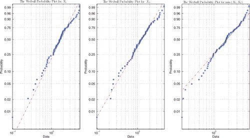
Naturally, we can choose the MOBW distribution to analyse the data. The estimates and 95% confidence (credible) intervals for the parameters are summarised in Table 6. From Table 6, it can be seen that the estimates of parameters are close to each other. Table 6 also shows that the shape parameter α > 1 which means the hazard rate function of the lifetime of the two eyes is increasing. Moreover, the failure probability of the laser-treated eye is much smaller than the untreated one, which indicates that the laser treatment has positive effect on delaying the onset of blindness in patients with diabetic retinopathy.

Table 6. The estimates of the parameters for the DRS data.

Method	α	95%CI	θ1	95%CI	θ2	95%CI	θ3	95%CP
MLE	1.558	(1.276,1.841)	0.469	(0.321,0.617)	0.394	(0.281,0.508)	0.465	(0.351,0.579)
ω1	1.557	(1.286,1.846)	0.471	(0.337,0.632)	0.393	(0.285,0.507)	0.462	(0.349,0.577)
ω2	1.557	(1.286,1.846)	0.471	(0.337,0.632)	0.396	(0.290,0.512)	0.460	(0.346,0.574)
ω3	1.549	(1.285,1.831)	0.477	(0.341,0.633)	0.391	(0.279,0.506)	0.464	(0.351,0.579)
ω4	1.549	(1.285,1.831)	0.477	(0.341,0.633)	0.393	(0.285,0.507)	0.462	(0.349,0.577)

8. Conclusion

In this paper, we have considered the dependent competing risks model by using an MOBW distribution. The objective Bayesian method is proposed to estimate the parameters. Based on different grouping orders, four reference priors are derived. Then the Bayesian approaches are compared with the maximum-likelihood method in terms of RMSE, RB and CP via a simulation study. The simulation results show that the Bayesian estimates perform better in terms of the CPs and RMSEs, and that we can choose a suitable reference prior to estimate the parameters according to the inferential importance.

Acknowledgments

The authors thank the editor-in-chief Dongchu Sun and the referee for their constructive suggestions that greatly improved the article.

Disclosure statement

No potential conflict of interest was reported by the authors.

Additional information

Funding

The research is supported by Natural Science Foundation of China [grant number 11671303], [grant number 11201345]; Natural Science Foundation of Zhejiang province [grant number LY15G010006]; China Postdoctoral Science Foundation [grant number 2015M572598].

Notes on contributors

Ancha Xu

Ancha Xu received the B.E. degree from the College of Mathematics and Statistics, Central China Normal University, Wuhan, China, and the Ph.D. degree from East China Normal University, Shanghai, China, in 2006 and 2011, respectively. He is currently an Associate Professor in the School of Mathematics and Information Science, Wenzhou University, Zhejiang, China. His research interests include Bayesian statistics, degradation modeling, and accelerated life testing.

Shirong Zhou

Shirong Zhou is currently working toward the Master degree in tSchool of Mathematics and Information Science, Wenzhou University, Zhejiang, China. His research interests include failure data analysis, accelerated life testing, and Bayesian inference.

Appendices

Appendix 1

A1. The reference prior of the MOBW distribution

Following the notions of Berger and Bernardo (1992), according to the inferential importance, we order a multi-dimensional parameter τ = (τ₁,… , τ_l) and separate it into m groups of sizes n₁, n₂,… , n_m, and these groups are given by where . Define then τ_{[ ∼ 0]} = τ and τ_[0] is vacuous.

The same as Berger and Bernardo (1992), the notation I(τ) is the Fisher information matrix and S(τ) = (I(τ))⁻¹. We will substitute I and S for I(τ) and S(τ) in the following sections.

Write S as so that A_ij is a n_i × n_j matrix, and define S_j = upper left (N_j × N_j) corner of S, with S_m = S, and H_j = S^{− 1}_j. Then the matrices play an importance role in deriving the reference priors. In particular, h₁ = H₁ = A^{− 1}₁₁ and, if S is a block diagonal matrix (i.e. A_ij = 0 for all i ≠ j), then h_j = A^{− 1}_jj, j = 1, …, m.

Lemma A.1:

If |h_j(τ)| depending only on τ_[j] holds, for j = 1,… , m, then the reference prior where |h_j(τ)| is the determinant of h_j(τ), τ* is any fixed point in Θ, and Θ is a compact subset.

One can refer to Berger and Bernardo (1992) for the proof. By using this lemma, the derivation of the m-group reference prior is greatly simplified.

There are four parameters in the MOBW distribution, in the following, we consider three cases, where the parameters are separated into two, three and four groups. We take {α, (θ₁, θ₂, θ₃)}, {(θ₂, θ₃), α, θ₁)} and {α, θ₁, θ₂, θ₃} as an example.

(I)	The reference prior of {α, (θ1, θ2, θ3)} is ω1(α, θ1, θ2, θ3).

Proof:

Based on the Fisher information matrix Σ, we can easily derive According to S_j = upper left (N_j × N_j) corner of S, H_j = S^{− 1}_j, we can obtain Due to h_j = lowerright (n_j × n_j) cornerof H_j, j = 1, 2, then

Choose Θ_k = Θ_1k × Θ_234k = {α|a_1k < α < b_1k} × {(θ₁, θ₂, θ₃)|a_2k < θ₁ < b_2k, a_3k < θ₂, a_4k < θ₃, θ₂ + θ₃ < d_k}, such that . Note that h₁ and h₂ satisfy Lemma A.1, then after some calculations, the reference prior for {α, (θ₁, θ₂, θ₃)} is

(II)	The reference prior of {(θ2, θ3), α, θ1} is ω1(α, θ1, θ2, θ3).

Proof:

The Fisher information matrix of {(θ₂, θ₃), α, θ₁} is Thus According to H_j = S^{− 1}_j, and h_j = lower right (n_j × n_j) corner of H_j, j = 1, 2, 3, we can obtained that , , H₃ = Σ₁. Then h₁ = H₁, , .

Choose Θ_k = {((θ₂, θ₃), α, θ₁)|a_1k < α < b_1k, a_2k < θ₁ < b_2k, a_3k < θ₂, a_4k < θ₃, θ₂ + θ₃ < d_k}, such that . According to Lemma A.1, it is not difficult to obtain that the reference prior for {(θ₂, θ₃), α, θ₁} is also

(III)

The reference prior of {α, θ1, θ2, θ3} is ω2(α, θ1, θ2, θ3).

Proof:

Due to S = Σ⁻¹, we can obtain Thus Then , , , .

Choose Θ_k = {(α, θ₁, θ₂, θ₃)|a_1k < α < b_1k, a_2k < θ₁ < b_2k, a_3k < θ₂, a_4k < θ₃, θ₂ + θ₃ < d_k}, such that . According to Lemma A.1, we can obtain the reference prior for {α, θ₁, θ₂, θ₃} is

The reference prior for π_u(α, λ₀, λ₁, λ₂) can be obtained from ω_u(α, θ₁, θ₂, θ₃), u = 1, 2, 3, 4, according to the one-to-one transformation from (α, λ₀, λ₁, λ₂) to (α, θ₁, θ₂, θ₃).

Appendix 2

Proving Theorem 5.1 needs the following two results (Guan et al., 2013): (B.1) (B.2) where B( ·, ·) is a beta function.

(I) The likelihood function under parameters (α, θ₁, θ₂, θ₃) is then the joint posterior distribution of (α, θ₁, θ₂, θ₃) under the prior ω₁ can be written as (B.3) Denote the right side of (B.3(B.3) ) as R, using (B.1(B.1) ), we have Denote then c is a constant. For any 0 < ϵ < 1, we have Obviously, where T_(n) is the largest order statistic of T_i, i = 1, 2,… , n, then R₃ < ∞. Thus Therefore, the posterior distribution of (α, θ₁, θ₂, θ₃) under the prior ω₁ is proper. Similarly, using (B.2(B.2) ), we can prove that the posterior distribution under the prior ω₂ is also proper.

(II) The posterior distribution of (α, θ₁, θ₂, θ₃) under the prior ω₃ iss (B.4) We denote the right side of (B.4(B.4) ) as P, using (B.2(B.2) ), we have denote then Q is a constant. For any θ₁ > 0, there exists a constant M₀ satisfying . Then according to (I), Therefore, Thus the posterior distribution of (α, θ₁, θ₂, θ₃) under the prior ω₃ is proper. Similarly, we can prove that the posterior distribution under the prior ω₄ is also proper.

References

- AL-Hussaini, E. K., Abdel-Hamid, A. H., & Hashem, A. F. (2015). Bayesian prediction intervals of order statistics based on progressively type-II censored competing risks data from the half-logistic distribution. Journal of the Egyptian Mathematical Society, 23, 190–196.
- Bemis, B., Bain, L. J., & Higgins, J. J. (1972). Estimation and hypothesis testing for the parameters of a bivariate exponential distribution. Journal of the American Statistical Association, 67, 927–929.
- Berger, J. O., & Bernardo, J. M. (1992). On the development of reference priors (with discussion). In J. M. Bernardo, J. O. Berger, A. P. Dawid, & A. F. M. Smith (Eds.), Bayesian statistics (Vol. 4, pp. 35–60). Oxford: Clarendon Press.
- Berger, J. O., Bernardo, J. M., & Sun, D. (2015). Overall objective priors (with discussion). Bayesian Analysis, 10, 189–221.
- Bernardo, J. M. (1979). Reference posterior distributions for Bayesian inference (with discussion). Journal of the Royal Statistical Society B, 41, 113–147.
- Cramer, E., & Schmiedt, A. B. (2011). Progressively type-II censored competing risks data from Lomax distributions. Computational Statistics and Data Analysis, 55, 1285–1303.
- Csorgo, S., & Welsh, A. H. (1989). Testing for exponential and Marshall-Olkin distribution. Journal of Statistical Planning and Inference, 23, 287–300.
- Dijoux, Y. D., & Gaudoin, O. (2009). The alert-delay competing risks model for maintenance analysis. Journal of Statistical Planning and Inference, 139, 1587–1603.
- Dimitrova, D. S., Haberman, S., & Kaishev, V. K. (2013). Dependent competing risks: Cause elimination and its impact on survival. Insurance: Mathematics and Economics, 53, 464–477.
- Feizjavadian, S. H., & Hashemi, R. (2015). Analysis of dependent competing risks in the presence of progressive hybrid censoring using Marshall-Olkin bivariate Weibull distribution. Computational Statistics and Data Analysis, 82, 19–34.
- Ghosh, J. K., & Mukerjee, R. (1991). Characterization of priors under which Bayesian and frequentist bartlett corrections are equivalent in the multiparameter case. Journal of Multivariate Analysis, 38, 385–393.
- Gilks, W. R., & Wild, P. (1992). Adaptive rejection sampling for Gibbs sampling. Applied Statistics, 41, 337–348.
- Guan, Q., Tang, Y. C., & Xu, A. C. (2013). Objective Bayesian analysis for bivariate Marshall-Olkin exponential distribution. Computational Statistics and Data Analysis, 64, 299–313.
- Jeffreys, H. (1961). Theory of probability. London: Oxford University Press.
- Kozumi, H. (2004). Posterior analysis of latent competing risk models by parallel tempering. Computational Statistics and Data Analysis, 46, 441–458.
- Kundu, D., & Dey, A. K. (2009). Estimating the parameters of the Marshall-Olkin bivariate Weibull distribution by EM algorithm. Computational Statistics and Data Analysis, 53, 956–965.
- Kundu, D., & Gupta, A. K. (2013). Bayes estimation for the Marshall-Olkin bivariate Weibull distribution. Computational Statistics and Data Analysis, 57, 271–281.
- Kundu, D., Kannan, N., & Balakrishnan, N. (2003). Analysis of progressively censored competing risks data. In N. Balakrishnan & C. R. Rao (Eds.), Handbook of statistics on survival analysis (Vol. 23, pp. 331–348). New York: Elsevier Publications.
- Laplace, P. (1812). Analytical theory of probability. Paris: Courcier Press.
- Lindqvist, B. H., & Skogsrud, G. (2009). Modeling of dependent competing risks by first passage times of Wiener processes. IIE Transactions, 41(1), 72–80.
- Marshall, A. W., & Olkin, I. (1967). A multivariate exponential distribution. Journal of the American Statistical Association, 62, 30–44.
- Mazucheli, J., & Achcar, J. A. (2011). The Lindley distribution applied to competing risks lifetime data. Computer Methods and Programs in Biomedicine, 104, 188–192.
- Pareek, B., Kundu, D., & Kumar, S. (2009). On progressively censored competing risks data for Weibull distributions. Computational Statistics and Data Analysis, 53, 4083–4094.
- Wang, C. P., & Ghosh, M. (2003). Bayesian analysis of bivariate competing risks models with covariates. Journal of Statistical Planning and Inference, 115, 441–459.
- Xu, A. C., Basu, S, & Tang, Y. C. (2014). A full Bayesian approach for masked data in step-stress accelerated life testing. IEEE Transactions on Reliability, 63, 798–806.
- Xu, A. C, & Tang, Y. C (2010). Reference analysis for Birnbaum-Saunders distribution. Computational Statistics & Data Analysis, 54, 185–192.
- Xu, A. C., & Tang, Y. C. (2011). Objective Bayesian analysis of accelerated competing failure models under type-I censoring. Computational Statistics & Data Analysis, 55, 2830–2839.
- Xu, A. C, Tang, Y. C, & Sun, D. C. (2015). Objective Bayesian analysis for masked data under symmetric assumption. Statistics and its Interface, 8, 227–237.
- Yang, R., & Berger, J. O. (1994). Estimation of a covariance matrix using the reference prior. The Annals of Statistics, 22, 1195–2111.