The influence of misspecified covariance on false discovery control when using posterior probabilities

ABSTRACT

This paper focuses on the influence of a misspecified covariance structure on false discovery rate for the large-scale multiple testing problem. Specifically, we evaluate the influence on the marginal distribution of local false discovery rate statistics, which are used in many multiple testing procedures and related to Bayesian posterior probabilities. Explicit forms of the marginal distributions under both correctly specified and incorrectly specified models are derived. The Kullback–Leibler divergence is used to quantify the influence caused by a misspecification. Several numerical examples are provided to illustrate the influence. A real spatio-temporal data on soil humidity is discussed.

Keywords:

• Multiple testing
• Bayes
• dependent data
• divergence
• spatio-temporal

1. Introduction

Large-scale multiple testing arises from many practical problems, from genetic studies to public health surveillance. Benjamini and Hochberg (1995) introduced the concept of the false discovery rate (FDR) and proposed a powerful testing procedure, usually referred as the BH procedure. The BH procedure relies on a positive dependence assumption (Benjamini & Yekutieli, 2001), while adaptive BH procedures (Liang & Nettleton, 2012; Storey, Taylor, & Siegmund, 2004) rely on an independence or weak dependence structure. Efron (2007) noted that correlation may result in overly liberal or overly conservative testing procedures. Though the BH procedure is valid under different dependence assumptions (Farcomeni, 2007; Wu, 2008), Sun and Cai (2009) showed that failing to model dependence can result in inefficiency. To address that problem, Sun and Cai (2009) and Sun, Reich, Cai, Guindani, and Schwartzman (2015) proposed a procedure using local significance index, which is a Bayesian posterior probability. Efron, Tibshirani, Storey, and Tusher (2001) described the connection between the FDR and Bayes procedures, where a posterior probability is referred as the local false discovery rate (Lfdr). Sun and Cai (2009)'s local significance index reduces to the Lfdr under independence. In fact, there is a rich history of using Bayesian approaches for multiplicity adjustment. Scott and Berger (2006) and Scott and Berger (2010) discussed Bayesian multiplicity adjustment in variable selections. Muller, Parmigiani, and Rice (2006) had a comprehensive discussion on the connection between the FDR, Bayesian multiple testing, and procedures using posterior probabilities.

In Sun et al. (2015), the procedure depending on unknown parameters is called the ‘oracle’ procedure, in the sense that we know all nuisance parameters as an oracle. Although the oracle procedure is proved to control FDR at the nominal level and be optimal in terms of false non-discovery rate (FNR), a data-driven ‘adaptive’ procedure relies on correctly specifying the model, including the prior specification, and/or consistent parameter estimation. For large-scale data, dependence or covariance, if in Gaussian models, is often estimated based on a structured model. The model choice or the structure choice itself may be debatable and parameter estimation remains challenging. For example, in spatial modelling, the estimation of covariance relies on structured covariance specifications and, in practice, one may have multiple choices of specifications. Intuitively, the choice of specification will influence the data-driven procedure and may eventually lead to different decisions.

In this paper, we explore the influence of a misspecified covariance structure on the testing procedure. Specifically, we study the sampling distributions of the Lfdr statistics under both correctly and incorrectly specified covariance structures. We derive explicit expressions for those distributions under a general model setting. We propose to use the Kullback–Leibler divergence as a quantitative measure for the influence. We show in both a simulation study and a real application that the influence of a misspecification leads to unappealing results. The paper is organised as follows. Section 2.1 gives a basic setup of this problem. Section 2.2 gives sampling distributions of the test statistics. Section 2.3 provides formulas for computing the Kullback–Leibler divergence. Section 2.4 shows several numerical examples. Section 3 provides real data that arose from the Oklahoma soil monitoring network. Section 4 is a discussion.

2. Main results

2.1. The setup

In this paper, we consider a general model for m observations : (1) where θ_i is the latent state and ε_i is the noise term which independently follows N(0, σ²). The dependence of observations is introduced through their latent states . For instance, θ_i can be a realised spatial process θ(s), for which a spatial dependence structure can be specified. Consider a one-sided hypothesis (2) for every i simultaneously. This type of one-sided hypothesis is often of interest in many practices. In spatial epidemiology, one may want to determine which regions or locations have disease rates higher than some given threshold θ₀. Here, data will be spatially correlated and each hypothesis will be one-sided. Similarly, in agricultural studies, one may want to determine which locations or time periods have soil moisture levels lower than a given threshold θ₀, indicating a risk of drought, and the data will be either spatially or temporally correlated and each hypothesis will be one-sided. A more general hypothesis would be H_0i : θ_i ∈ Θ_0i versus H_1i : θ_i ∈ Θ_1i. We do not consider a precise (or two-sided) hypothesis in this paper, but some comments are given in Section 4.

The dependence of latent states is usually specified through a prior model. For example, consider a normal-inverse-gamma prior on , (3) For simplicity, we assume that is a known covariance structure and g is a known scale parameter. The use of g here is the same as that in Zellner's g-prior for Bayesian variable selection problems. The g value could be fixed, estimated or have a hyperprior (Liang, Paulo, Molina, Clyde, & Berger, 2008). The prior specification (3(3) ) in fact induces a marginal probability for each hypothesis: P(H_0i) = P(θ_i ≥ θ_0i) = 0.5.

Sun and Cai (2009) and Sun et al. (2015) showed that, to control FDR when data are dependent, the posterior probability is useful. The posterior probability h_i is viewed as a test statistic, called local index of significance in their work. The oracle procedure orders and rejects all H_(i), i = 1,… , k such that (4) where α^* is the nominal level. The procedure mimics the Benjamini–Hochberg procedure, in which p-value is the test statistic. Sun and Cai (2009) showed that this oracle procedure controls FDR at level α^* and has the smallest FNR among all FDR procedures at α^* for a hidden Markov model. Sun et al. (2015) further showed that in a spatial random field model, this oracle procedure controls FDR at level α^* and has the smallest missed discovery rate (MDR). A data-driven procedure, however, depends on the estimation of other nuisance parameters. The covariance is especially important in this case as it describes the dependence. Our objective is to determine if the procedure is sensitive when the covariance is incorrectly specified or estimated, and, if so, to quantify the sensitivity.

2.2. Sampling distribution of test statistics

2.2.1. Known variance of noise

We now focus on how the distribution of test statistics (h₁,… , h_m) is influenced by a misspecified covariance structure. Assume that the data are generated from the true underlying process: (5) for i = 1,… , m. Assume known σ²₀ and consider model (1(1) ) with priors and , the latter of which has a misspecified covariance structure. The scale g determines the strength of the prior. The intuition is that both g and will influence the test statistics (h₁,… , h_m) and FDR control.

Lemma 2.1:

Under the correct covariance , h_i marginally has the following CDF: (6) where a_ii is the ith diagonal element in and b_ii is the ith diagonal element in .

Under the misspecified covariance , and .

Lemma 2.1 shows explicitly how the sampling distribution is altered by a misspecification. Observe that F(h_i) is completely determined by the ratio a_ii/b_ii. Figure 1 shows different shapes of both cumulative distribution functions (CDF) and probability density functions (pdf) under different ratio values. Note that when a_ii = b_ii, the sampling distribution is Uniform(0, 1). Consider g → ∞, for which the prior becomes noninformative, then a_ii/b_ii → σ²₀/(σ²₀ + σ²_{1, ii}), where σ²_{1, ii} is the ith diagonal element in . The ratio becomes irrelevant to the misspecified covariance . In other words, the behaviours of the correct specification and the incorrect specification will be similar when g is large, which seems intuitive. Because FDR procedures based on h_i reject H_0i if h_i ≤ C for some C, it is important to note that P(H_i ≤ h_i) = F(h_i) can be substantially influenced by covariance misspecification. For example, in Figure 1, we see F(0.2) ranges from 0.03 to 0.35. It should be noted that some recommend rejecting H_0i if h_i ≤ 0.2 (Efron, 2012). In this setting, the rejection probability ranges from 0.03 to 0.35.

Figure 1. Marginal CDF and pdf for h_i.

Unlike the independent case, h₁,… , h_m are now dependent when the data are dependent. The change under a misspecified structure is revealed in their joint distribution.

Theorem 2.1:

Using the same definition for and in Lemma 2.1, h₁,… , h_m have a joint CDF where Φ^m_b is the CDF for a multivariate normal , and is the correlation matrix of .

The joint distribution of h₁,… , h_m represents a multivariate surface in the space [0, 1]^m. Notice that jointly not only the ratio a_ii/b_ii plays a role but also the correlation structure of . Under a misspecified covariance structure, will be altered as well. However, still, as g → ∞, , and there is no misspecification effect.

2.2.2. Unknown variance of noise

Assume the underlying data-generating process (5(5) ). Suppose σ²₀ is unknown and consider specifying model (1(1) ) with prior (3(3) ). As before, a correct covariance structure is and a misspecified structure is .

Theorem 2.2:

Under the correct covariance , the test statistics h₁,… , h_m jointly have the following CDF: (7) where , , Ψ_{m + 2α} is the CDF for a univariate t-distribution with degrees of freedom m + 2α, and Ξ^m_{a, b} is the CDF for the following random vector where and , where here denotes a diagonal matrix.

Under the misspecified covariance , and .

The main difference between Theorem 2.2 and Theorem 2.1 is that Ξ^m_{a, b} has a more complicated form than Φ^m_b. The ratio a_ii/b_ii still plays a role in the joint distribution and Ξ^m_{a, b} will be affected by a misspecified structure.

2.3. Kullback–Leibler divergence

Denote the sampling distribution of under the correct covariance specification as and under the misspecified covariance as . We evaluate the influence of the misspecification by the Kullback–Leibler (KL) divergence (8) The KL divergence here can be interpreted as the information loss when using f_mis to approximate f_cor. The following two corollaries are useful to approximate the KL divergence in our cases.

Corollary 2.1:

As a consequence of Lemma 2.1, the marginal density function of h_i is where r_i = a_ii/b_ii and φ_i = Φ⁻¹(h_i).

Corollary 2.2:

As a consequence of Theorem 2.1, the joint density function of (h₁,… , h_m)′ is where and .

With Corollary 2.2, the term in expression (8(8) ) is analytically available. Thus, the KL divergence D_KL can be easily evaluated using Monte–Carlo approximation. Notice that we can draw from f_cor exactly given the underlying model because is analytically available. To draw a sample of from f_cor, draw from the underlying model and then calculate . Suppose we obtain a sample , the approximation is A misspecified covariance will change the defined matrices and , and consequently change matrices and . Notice the relationship . Since the KL divergence will generally increase as the dimension m increases (in the independent case, it is simply a sum of individual dimensions), we may also consider a relative measure of influence D_KL/m.

The KL divergence is computable under the general model (1(1) ) with and provided. This easy-to-compute measure can be used to quantify the influence of a misspecification. In practice, when there are multiple candidate covariances, we may assess the KL divergence between those candidates.

2.4. Numerical examples

We now consider two examples of misspecified covariance. In each example, without loss of generality, we set m = 900 and σ²₀ = 0.25. We will numerically evaluate the KL divergence and perform a simulation study, in which we estimate FDR and FNR with Monte–Carlo replications of 1000.

Example 2.1:

Positive spatial covariance vs. Independence.

Consider a regular spatial grid with unit distance one for generating the latent states . The true covariance has a positive decaying structure determined by an exponential covariance function σ²_{1, ij} = exp { − ‖s_i − s_j‖/ρ} with ρ = 5, where s represents a location. A misspecified covariance is . To get a rough idea of r_i = a_ii/b_ii, let g = 1 and compute and . Under the correct specification, r_i ranges from 0.12 to 0.16, and under the misspecification, r_i = 0.25.

Note that this misspecification is essentially to ignore the dependence and treat data as independent observations. This is quite common in practice, where domain scientists are hesitant to model complex covariance structures, though evidences suggest that data may be correlated.

Example 2.2:

Negative AR(2) covariance vs. Positive AR(2) covariance.

Consider a time series for generating the latent states . The true covariance is determined by an AR(2) process: θ_i = ρ₁θ_{i − 1} + ρ₂θ_{i − 2} + ϵ_i, ϵ_i ∼ N(0, 1), and ρ₁ = 1.5 and ρ₂ = −0.9. The autocorrelation function of this specification has an oscillating pattern (mixed positive and negative values in ). A misspecified covariance is chosen to be the covariance for an AR(2) process with ρ₁ = 0.6 and ρ₂ = 0.3, whose autocorrelation is always positive. To get a rough idea of r_i = a_ii/b_ii, let g = 1 and compute and . Under the correct specification, r_i ranges from 0.088 to 0.14, and under the misspecification, r_i ranges from 0.20 to 0.25.

Note that this example shows a scenario where model is correctly specified but parameter estimates are wrong. This example also compares a covariance matrix containing negative values with a covariance matrix containing all positive values.

Results of Examples 2.1 and 2.2 are shown in Figures 2 and Figure 3. We choose different g values representing different strengths of information brought in by the prior dependence. Four plots are shown in each result: the estimated FDR, the estimated FNR, the difference between the rejection rate of the correct specification and that of the misspecification, i.e., , and D_KL/m. We can reach the following conclusions from these plots. First, as g increases, both the KL divergence and the difference between rejection rates decrease, and also both the FDR and the FNR become closer, all of which are as expected, indicating a decreasing misspecification influence. Second, the FNR under the misspecification is universally higher than under the correct specification. Hence, misspecification results in an inefficient procedure. Also notice that the procedure tends to give less discoveries under the misspecification than under the correct specification. Last but not least, the FDR change is not monotonic and the comparison between the two specifications is profound. Notice that the nominal level is 0.05 and g = 1 (or log₁₀g = 0) represents a ‘true’ scale. When both the structure and the scale g are correct, from the top left plot in both results, we can see that the FDR is controlled at the nominal level. This seems to suggest that a correctly estimated scale of prior dependence is desired, which should be neither too strong nor too weak. And this correct scale will only work as expected if the covariance structure is correct as well.

Figure 2. Results for Example 2.1. FDR, FNR, difference of rejection rate (rate_cor − rate_mis) and D_KL/m. The sequence of g is from 0.2 to 500. The nominal level is 0.05.

Figure 3. Results for Example 2.2. FDR, FNR, difference of rejection rate (rate_cor − rate_mis) and D_KL/m. The sequence of g is from 0.2 to 500. The nominal level is 0.05.

Example 2.3:

Positive spatial covariance revisit.

Revisit Example 2.1. Consider to fix g = 1. The correct specification is exactly the same as the underlying model with ρ = 5. For the misspecification, let the spatial range parameter ρ change from 0.1 to 20, representing the strength of dependence.

Results of Example 2.3 are shown in Figure 4. The FDR is maintained at 0.05 only when ρ has the correct value. The pattern of change in FDR is also reflected in the KL divergence plot. In this example, using D_KL/m as a measure of influence seems to be reasonable. The FNR, on the other hand, monotonically decreases as the dependence goes stronger. We shall note here that, when g is large, the KL divergence becomes sensitive to detect a misspecification as the measure approaches zero. However, in that case, the prior is vague and the influence on FDR is negligible.

Figure 4. Results for Example 2.3. FDR, FNR and D_KL/m. The dashed vertical line is the correct value ρ = 5. The sequence of ρ is (0.1, 0.5, 1, 5, 10, 20). The nominal level is 0.05.

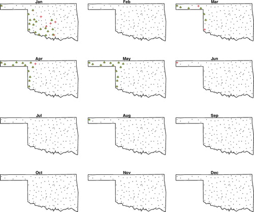
Figure 5. Rejected sites for the year of 2014 in Oklahoma, from January to December. The dots (·) are the observations, the crosses (+) are rejections using Model 1, and the triangles (▵) are rejections using Model 2.

3. Real data: soil relative humidity

Oklahoma Mesonet (Illston et al., 2008) is a comprehensive observatory network monitoring environmental variables across the state. One of the focuses of the network is soil moisture. Extreme weather conditions, especially drought, severely impact Oklahoma's agriculture, which is a leading economy of the state. Soil moisture is fundamentally important to many hydrological, biological and biogeochemical processes. The information is valuable to a wide range of government agencies and private companies. We take a small dataset from their data warehouse as an example of real application. Consider only one variable here: the relative humidity, ranging from 0% to 100%. The dataset consists of monthly averages in 2014 for 108 monitoring stations, which is in total 1296 measurements. Consider each hypothesis being H_0i : θ_i ≥ 50 versus H_0i : θ_i < 50 for detecting low humidity times and locations.

We consider two different specifications for the dependence structure. Consider a spatio-temporal process, for a spatial location and a time point t, , where is pure error process with N(0, σ²), and is a stationary Gaussian process with a constant mean μ and a separable covariance function: where and τ = |t − t′| are both Euclidean distances. Specify C^(s)(h) = exp {−h/ρ} and C^(t)(τ) = α^τ. Specify priors for parameters: σ² ∼ IG(1, 1), δ ∼ IG(1, 1), ρ ∼ Uni(0, +∞) and α ∼ Uni(0, 1). Posterior distributions are obtained through standard Markov chain Monte–Carlo (MCMC). We ensure that the chain is long enough to converge and take 10,000 MCMC samples. Posterior probabilities are approximated with posterior samples.

The second model is specified that the process is independent over time but the variance is not stationary over time: This is a different specification from Model 1 and neither model is a reduced case of the other. We use the same specification for C^(s)(h) as in Model 1 and also the same prior distributions for σ², δ_t and ρ. We take 10,000 MCMC samples and posterior probabilities are approximated with MCMC samples.

For both models, we follow the FDR control procedure (4(4) ) at a nominal level 0.05. Results of both are shown in Figure 5. Note that drought impacts Oklahoma mostly in the western areas. Both results seem reasonable and meaningful for practitioners and they overlap on most decisions. However, we do observe that, at nine time/location points, they do not agree with each other. Those nine points are all rejected in Model 1 but neither in Model 2. Table 1 shows the observed values for the nine disagreed sites, along with their upper credible intervals inferred from each model. We can see that all nine points are boundary cases and Model 2 results in higher upper bounds than Model 1, causing the disagreed decisions. Such disagreed decisions will likely cause confusions in practice. As one must assume normality in the first place before performing a small sample t test, we believe that, in a good practice, it is necessary to clearly assume and carefully check the model specification before using posterior probabilities from the model for testing.

Table 1. Soil data: disagreed decisions under Models 1 and 2, for hypothesis H_0i : θ_i ≥ 50 versus H_0i : θ_i < 50.

Time and	Observed	Upper C.I.	Upper C.I.
location	value	under Model 1	under Model 2
January, Site 6	49.49	50.42^a	51.03
January, Site 70	49.55	50.52^a	51.30
January, Site 72	49.62	50.37^a	50.89
January, Site 87	49.70	50.67^a	51.07
January, Site 101	49.62	50.70^a	51.21
March, Site 8	49.94	50.78^a	51.10
March, Site 47	49.58	50.36^a	51.22
April, Site 38	49.53	50.19^a	50.90
June, Site 53	49.63	50.85^a	51.83

^aA rejection under the model. The nominal level is 0.05.

4. Discussion

In this paper, we explore the influence of a misspecified covariance structure on the multiple testing procedure using Bayesian posterior probabilities. We explicitly show the influence on the test statistics and discuss the KL divergence as a measure of that influence. We see from a simulation study that both the correct strength of dependence and structure of dependence are necessary to ensure control of the FDR at the nominal level. We also see that misspecified covariance can significantly impact efficiency, in terms of FNR. From a real application, we see that different covariance specifications can result in different decisions.

This paper does not cover any discussion on a precise (or two-sided) hypothesis: H_0i : θ_i = 0 versus H_1i : θ_i = 0. In that scenario, a mixture model is often assumed: f(y) = p₀f₀(y) + p₁f₁(y). The Lfdr by Efron et al. (2001) is p₀f₀(y)/f(y) under independence. When data are dependent, it is unclear how to properly incorporate the dependence into the mixture model. One practical example given by Brown, Lazar, Datta, Jang, and McDowell (2014) specifies: y_i ∼ N(γ_iμ_i, σ²), γ_i ∼ Bern(1 − p) and , which mimics the independent model in Scott and Berger (2006). In the Bayesian framework, to compute , we would need P(H_0i), P(H_1i) and priors π_i0(θ_i) under H_0i and π_i1(θ_i) under H_1i. Moreover, π_i0(θ_i) and π_i1(θ_i) should have a dependence structure for i = 1,… , m, in some way. A misspecified covariance (or model) would be worth further investigation in this setting.

Disclosure statement

No potential conflict of interest was reported by the authors.

Additional information

Funding

This research is partially supported by National Science Foundation [grant number OIA-1301789].

Notes on contributors

Ye Liang

Ye Liang is an assistant professor in the Department of Statistics at Oklahoma State University, USA. His research areas include Bayesian statistics and spatial statistics. He primarily focuses on applications in ecological, agricultural and environmental studies, and biomedical and healthcare studies.

Joshua D. Habiger

Joshua D. Habiger is an associate professor in the Department of Statistics at Oklahoma State University, USA. His research interests include high dimensional statistical inference and categorical data analysis.

Xiaoyi Min

Xiaoyi Min is an assistant professor in the Department of Mathematics and Statistics at Georgia State University. His research interests include Bayesian statistics, statistical genetics and meta-analysis.

Appendix

A.1 Proof of Lemma 2.1

Proof:

First, given the underlying true model (5(5) ), it is straightforward to derive the true marginal distribution for : (A1) If we estimate the posterior using the correct covariance structure, we will have the following posterior distribution: , where and . Marginally, . Then, Using (A1(A1) ), we have the marginal distribution: , where . Note that is free of , so let . Marginally, θ^(y)_i ∼ N(θ_0i, b_ii) which leads to Now, under the true covariance, the CDF for H_i is given by If a misspecified covariance is used to estimate the posterior, then in the posterior distribution , we will have , instead of in both and . As a consequence, and . The rest remains the same.

A.2 Proof of Theorem 2.1

Proof:

According to the proof in Lemma 2.1, . Hence, , where is the correlation matrix of . Equivalently, Then, the joint CDF of (H₁,… , H_m)′ is

A.3 Proof of Theorem 2.2

Proof:

First, given the underlying true process (5(5) ), marginally, .

If the correct covariance is used, we have the posterior distribution which is , with location and scale . Similarly as Lemma 2.1, define and .

Marginally, , then each test statistic is In order to find the joint CDF, we need the joint distribution of , which can be re-written as (A2) Given the marginal distribution of , we have , or, . The quadratic term in (A2(A2) ) is Equation (A2(A2) ) is then Or, equivalently, The joint CDF of H₁,… , H_m is given by If the misspecified covariance is used, follow the same argument in Lemma 2.1.

A.4 Proof of Corollary 2.1

Proof:

Notice that dΦ⁻¹(x)/dx = 1/ϕ(Φ⁻¹(x)), where . Then,

A.5 Proof of Corollary 2.2

Proof:

Let . Using the chain rule,

References

- Benjamini, Y., & Hochberg, Y. (1995). Controlling the false discovery rate: A practical and powerful approach to multiple testing. Journal of the Royal Statistical Society, Series B, 57, 289–300.
- Benjamini, Y., & Yekutieli, (2001). The control of the false discovery rate in multiple testing under dependency. Annals of Statistics, 29, 1165–1188.
- Brown, A., Lazar, N., Datta, G., Jang, W., & McDowell, J. (2014). Incorporating spatial dependence into Bayesian multiple testing of statistical parametric maps in functional neuroimaging. Neuroimage, 84, 97–112.
- Efron, B. (2007). Correlation and large-scale simultaneous significance testing. Journal of the American Statistical Association, 102, 93–103.
- Efron, B. (2012). Large-scale inference: Empirical Bayes methods for estimation, testing and prediction. Cambridge, UK: Cambridge University Press.
- Efron, B., Tibshirani, R., Storey, J., & Tusher, V. (2001). Empirical Bayes analysis of a microarray experiment. Journal of the American Statistical Association, 96, 1151–1160.
- Farcomeni, A. (2007). Some results on the control of the false discovery rate under dependence. Scandinavian Journal of Statistics, 34, 275–297.
- Illston, B., Basara, J., Fisher, D., Elliott, R., Fiebrich, C., Crawford, K.,… Hunt, E. (2008). Mesoscale monitoring of soil moisture across a statewide network. Journal of Atmospheric and Oceanic Technology, 25, 167–182.
- Liang, F., Paulo, R., Molina, G., Clyde, M., & Berger, J. (2008). Mixtures of g priors for Bayesian variable selection. Journal of the American Statistical Association, 103, 410–423.
- Liang, K., & Nettleton, D. (2012). Adaptive and dynamic adaptive procedures for false discovery rate control and estimation. Journal of the Royal Statistical Society, Series B, 74, 163–182.
- Muller, P., Parmigiani, G., & Rice, K. (2006). FDR and Bayesian multiple comparisons rules. Proceedings of Valencia/ISBA 8th world meeting on Bayesian statistics, Benidorm, Alicante, Spain.
- Scott, J., & Berger, J. (2006). An exploration of aspects of Bayesian multiple testing. Journal of Statistical Planning and Inference, 136, 2144–2162.
- Scott, J., & Berger, J. (2010). Bayes and empirical-Bayes multiplicity adjustment in the variable-selection problem. The Annals of Statistics, 38, 2587–2619.
- Storey, J., Taylor, J., & Siegmund, D. (2004). Strong control, conservative point estimation and simultaneous conservative consistency of false discovery rates: A unified approach. Journal of the Royal Statistical Society, Series B, 66, 187–205.
- Sun, W., & Cai, T. (2009). Large-scale multiple testing under dependence. Journal of the Royal Statistical Society, Series B, 71, 393–424.
- Sun, W., Reich, B., Cai, T., Guindani, M., & Schwartzman, A. (2015). False discovery control in large-scale spatial multiple testing. Journal of the Royal Statistical Society, Series B, 77, 59–83.
- Wu, W. (2008). On false discovery control under dependence. Annals of Statistics, 36, 364–380.