Semiparametric Bayesian analysis of high-dimensional censored outcome data

ABSTRACT

The Surveillance, Epidemiology and End Results (SEER) cancer database contains survival data for US individuals diagnosed with cancer. Semiparametric Bayesian methods are computationally expensive to fit for such large data-sets. This paper develops a cost-effective Markov chain Monte Carlo strategy for censored outcomes to fit a semiparametric bayesian analysis of SEER data of New Mexico. We use an accelerated failure time model, with Dirichlet process random effects for inter-subject variation, and intrinsic conditionally autoregressive random effects for spatial correlations. The results offer insights into differences in breast cancer mortality rates between ethnic groups, tumor grade and spatial effect of counties.

Keywords:

• ICAR models
• data squashing
• Dirichlet process
• generalised Pólya urn process
• big data

1. Introduction

Large data-sets of censored outcomes have become commonplace. For instance, the Surveillance, Epidemiology and End Results (SEER) database contains survival outcome data for US individuals diagnosed with cancer. Moreover, it has become routine to analyse survival outcome data-set using Bayesian models that investigate complex relationships between cancer survival and covariates such as race, etc.

Ideally, researchers should exploit the richness of large databases to gain new insights. However, the challenge of processing massive amounts of data poses a bottleneck. This paper attempts to tackle some of these challenges and fits flexible but readily interpretable semiparametric accelerated failure time (AFT) model for large censored outcome data-sets such as SEER.

We focus on 26,285 New Mexican women who were diagnosed with breast cancer between 1973 and 2012, and were either African American, white, or American Indian. The data was released by SEER in November 2014. The subject-specific responses was survival time in months (see SEER Research Data (1973–2012)).

Covariate information for each subject includes (i) patient race: race_i, coded as 1, 2, or 3 if the person is white, African American, or American Indian, (ii) calendar year of diagnosis: year_i, ranging from 1973 to 2012, (iii) patient age at diagnosis: age_i, ranging from 19 to 101 years, (iv) tumor grade: grade_i = 1, 2, 3, or 4, corresponding to tumors ordered from well-differentiated to poorly differentiated and (v) Five-digit Federal Information Processing Standard (FIPS) county code of residence at diagnosis, denoted by j = j(i), representing the 33 counties of New Mexico.

Semiparametric Bayes methods for spatially correlated survival data.    There is vast literature on existing methods. For comprehensive discussions, refer to Ibrahim, Chen, and Sinha (2001), Hanson, Jara, and Zhao (2011), Nieto-Barajas (2013), Müller, Quintana, Jara, and Hanson (2015), Zhou and Hanson (2015). Briefly, the methodological background is as follows. Cox (1975) introduced proportional hazards (PH) models. Kalbfleisch (1978), Gelfand and Mallick (1995), Carlin and Hodges (1999), Hennerfeind, Brezger, and Fahrmeir (2006), Hanson (2006), Hanson and Yang (2007), Kneib and Fahrmeir (2007), Zhao, Hanson, and Carlin (2009) developed various Bayesian semiparametric approaches to PH models. Frequentist AFT models for right-censored data were introduced by Buckley and James (1979). Kuo and Mallick (1997), Walker and Mallick (1999), Kottas and Gelfand (2001), Hanson and Johnson (2002), Hanson (2006), Hanson and Yang (2007), Komárek and Lesaffre (2007), Komárek and Lesaffre (2008), Zhao et al. (2009) developed semiparametric Bayes versions of AFT model; these approaches were based on Dirichlet process (DP) mixture models, finite mixtures of normal distributions, approximating B-splines, and Polya tree priors. Although AFT models are less frequently used than PH models, investigations have demonstrated that AFT models provide much better fit and interpretability in applications, e.g. see Hanson and Yang (2007), Hanson (2006), Kay and Kinnersley (2002). For these reasons, we fit the SEER breast cancer data using AFT models.

When censored outcomes are spatially correlated, the spatial dependence is analysed after adjusting for other covariate effects. There are two main approaches for incorporating spatial dependence in semiparametric models: frailty and copula. See Li and Ryan (2002), Banerjee, Carlin, and Gelfand (2015), Zhou and Hanson (2015). For areal level data, such as SEER datasets which have individual counties of residence at diagnosis, intrinsic conditionally autoregressive (ICAR) model of Besag, Mollie, and York (1991) is often applied (Banerjee, Wall, & Carlin, 2003; Pan, Cai, Wang, & Lin, 2014; Zhao et al., 2009).

There is an increasing number of approaches for modelling spatially correlated survival data using semiparametric methods (Banerjee et al., 2015; Banerjee et al., 2003; Diva, Banerjee, & Dey, 2007; Li & Ryan, 2002; Pan et al., 2014; Zhou & Hanson, 2015; Zhao et al., 2009; Zhou & Hanson, 2017). Most approaches have proposed spatially varying frailties in the conditional PH set up. For instance, Diva et al. (2007) models the baseline hazard function as mixtures of beta distributions and models spatially varying frailities by putting a multivariate conditionally autoregressive prior on spatial frailties. Zhao et al. (2009) models the baseline hazard function for every region as mixture of polya tree prior and the dependence is induced between baseline hazard function of neighbouring regions. Recently, Zhou and Hanson (2017) proposed a method, in which, they put a Transformed Bernstein Polynomial (TBP) prior on the baseline survival function of AFT model.

In the light of preceeding discussions, we take a different approach. This paper proposes an AFT model in semiparametric framework to analyse spatially correlated survival data. Fixed effects account for subject-specific covariates such as age and race. We apply the approach of Kuo and Mallick (1997) for censored outcomes, the residual individual variation in mortality rate is modeled using DP mixture random effects (Antoniak, 1974; Blackwell & MacQueen, 1973; Ferguson, 1973; Freedman, 1963; Ghosal, Ghosh, & Ramamoorthi, 1999; Ishwaran & Zarepour, 2002; Neal, 2000; Sethuraman, 1994; Sethuraman & Tiwari, 1982). Additionally, the spatial correlation in responses is modelled using ICAR model Besag et al. (1991). The novelty of our approach lies in relaxing the assumption of AFT model by incorporating random intercept for residual individual variation and including spatial frailties. The advantage of our approach is that model parameters are easier to interpret but at the same time our model is more flexible compared to AFT model. Furthermore, we also propose a fast sampling method which can reduce the computational cost of our method.

The computational cost of Big Data.    The posterior distribution of proposed model, see Section (2), is analytically intractable. Since the model is conditionally conjugate in the DP random effects, we could potentially apply a Gibbs sampler (Bush & MacEachern, 1996; Escobar, 1994; Escobar & West, 1995; MacEachern, 1994; West, Müller, & Escobar, 1994). However, Gibbs samplers for DP random effects are computationally expensive for large data-set.

To fit flexible Bayesian models on large data-sets, we require efficient strategies. Several data squashing strategies have been developed over the years. For instance, Blei and Jordan (2005) introduced a variational inference method for DP models; and Pennell and Dunson (2007) developed an empirical Bayes approach for DP models. Guha (2010) proposed a general MCMC technique capable of quickly and accurately investigating the posterior in a large class of Bayesian semiparametric models.

However, the above data-squashing techniques are not directly applicable to survival datasets. To fill this gap, we adapt the ideas of Guha (2010) to devise a MCMC algorithm designed for the Bayesian analyses of large censored outcome data-sets. The resultant inferences are from the exact posterior distribution rather than an approximation.

The rest of the paper is organised as follows. Section 2 specifies the proposed model and Section 3 describes a fast inference strategy for large censored databases. Section 4 analyses simulated survival data to demonstrate the reliability of Section 3 strategy. Section 5 presents the results for the New Mexico breast cancer data. Finally, Section 6 ends the paper with discussion.

2. Model

For individuals indexed by i = 1,… , n, let y_i denote the survival time. Let δ_i = 0 (1) indicate whether time y_i is right-censored (not censored). Writing z_i = log y_i, and assuming that the censoring and failure times are independent, the likelihood contribution of subject i in an AFT model is (1) where φ( · ∣μ_i, σ²) denotes normal density with mean μ_i and variance σ², and S( · ∣μ_i, σ²) denotes survivor function. A small value of ε results in a vague prior for parameter σ².

An equivalent approach relies on possibly latent log-failure times, t_i, and independently distributed log-censoring times, c_i: (2) (3) Subject-specific normal means.    Suppose all covariates except the areal units are contained in a vector of length p ∀ i = 1,… , n. Let the areas be labelled {1,… , J}, with j = j(i) denoting the area associated with subject i at diagnosis. Then, subject-specific mean μ_i is given as (4) where is a vector of p fixed effects, η_j is j^th area's random effect, and θ_i denotes the residual individual variability. Vague normal priors are assumed for the fixed effects.

New Mexico breast cancer analysis.    For SEER application, mean μ_i is assumed to be a linear function of covariates such as age etc, as shown below: (5) where β₀ is intercept, β₁ is the effect of age at diagnosis, β₂ is the effect of calendar year of diagnosis, is the factor effect of race (with whites as reference group), and is the factor effect of tumor grade at diagnosis (with well-differentiated tumors as reference group).

Area-specific random effects. Let be vector of area-specific random effects in expressions (4(4) ) and (5(5) ). The ICAR model of Besag et al. (1991) generally defines ‘neighbours’ as areal units that share a nontrivial border containing more than one point on the map. Let the symbol indicate that counties s and t are neighbours. Let m_s be the number of spatial neighbours of county s. Define J by J matrix with elements for s, t = 1,… , J, with I( · ) denoting the indicator function.

The model assumes that vector of areal random effects, , has a multivariate normal prior with mean and covariance matrix whose Moore-Penrose generalised inverse is . Parameter σ²_η is given an inverse gamma prior. Although the ICAR prior is improper, the posterior is proper, and valid Bayesian inferences are therefore obtained.

Individual random effects.   Let represent the DP with base distribution H and mass parameter M > 0. Assume the following prior for subject-specific random effects appearing in Equations (4(4) ) and (5(5) ): (6) Hyperparameter α is given a vague prior.

Applying the stick-breaking representation (Sethuraman, 1994; Sethuraman & Tiwari, 1982), the random distribution P in Equation (6(6) ) is written as where the distinct atoms θ*_j are iid N(0, τ²). Furthermore, the probability weights have the expression: p₁ = V₁, and p_j = V_j ∏_{k < j}(1 − V_k) for j > 1, where . In particular, random distribution P is almost surely discrete.

Another representation of DP prior was given by Blackwell and MacQueen (1973). The representation of the prior distribution of θ_i is given in terms of successive conditional distributions, which is given as below. (7)

The above equation allows θ_i to share the same value as that of any of the previous θ_k, where k =1…i − 1 or draw a new value from the discrete distribution P. Thus, The DP prior allows n subjects to cluster in all possible ways. Let θ*₁, …, θ_K* be the distinct random effects of n subjects, and let n_j be the number of subjects belonging to j^th cluster (i.e. subjects for which θ_i = θ*_j). The joint distribution of random effects induced by DP prior (6(6) ) is then (8)

Define the residual error distribution, F, as the random distribution P with additive Gaussian white noise: (9) where * denotes convolution. Then the (possibly latent) log-failure times t_i of the n individuals are iid F, provided the fixed effects and spatial random effects in Equations (4(4) ) and (5(5) ) are equal to 0. The residual error distribution is interpreted as the variability in log-survival time that cannot be explained by covariates. Ghosal et al. (1999) have shown that, as n grows, the true residual error distribution is consistently estimated by model (6(6) ). This motivates the use of semiparametric approaches for large datasets.

3. Posterior inference for high-dimensional censored outcome databases

Guha Guha (2010) proposed a strategy applicable to generalised Polya urn processes (GPUs), a broad class of parametric and semiparametric mixture models. The key idea is to identify ‘δ-neighbourhoods’ of subjects having similar full conditionals. This results in drastic reductions in the effective number of subjects, and hence, computational costs of updates. Guha Guha (2010) proved that this strategy yields unbiased MCMC posterior inferences in GPUs. Here, we adapt the technique to devise an MCMC algorithm for Section 2 model and censored outcomes.

3.1. Fast MCMC algorithm for DP random effects

Suppose that failure times t₁,… , t_n, fixed effects , ICAR random effects , and other hyperparameters are equal to their current MCMC values. Conditional on these parameters, we efficiently generate the DP random effects of n individuals.

For an integer q, vectors and index set I⊂{1,… , q}, let symbol denote the set of vectors,

. Let denote the K distinct atoms, . For i = 1,… , n, define a discrete random variable c_i taking values 1,… , K, and having probability mass function given by (10) where b_i is the normalising constant. Mass function (10(10) ) is designed to closely approximate the full conditional of θ_i when n is large; see Guha (2010). Furthermore, they have lower computational cost than full conditionals.

MCMC updates of    Let δ be a user-specified input parameter controlling the size of δ-neighbourhoods. For our analysis, we fixed the value of δ as 0.1. The MCMC update proceeds as follows:

(1)

Initialise set R = {1, 2,… , n}.

(2)

Repeat following steps until set R is empty: (a) Let be the current random effects of n individuals. (b) Randomly pick a subject i from R. (c) For k ∈ R, compute the mass functions using definition (10(10) ). For fixed i, evaluate |R| squared Hellinger distances between the discrete distributions and for k ∈ R: Recall that squared Hellinger distances belong to the interval [0, 1]. (d) Identify a δ-neighbourhood of subjects, D, as follows: The remaining sub-steps jointly update the vector consisting of the random effects for the entire δ-neighbourhood. (e) Let set be the complement of δ-neighbourhood D. For subjects belonging to (i.e., do not belong to the δ-neighbourhood), inspect their random effects, to compute the following quantities that will be useful in the sequel. Let set contain the number of distinct values among the random effects . For , let be the number of subjects belonging to sharing the common value . (f) Let ξi be a discrete random variable taking values in the set : (g) Generate allocation variables for δ-neighbourhood D: (h) Compute the set D0 = {k: k ∈ D, sk = 0}. This represents the δ-neighbourhood members whose random effects do not belong to the set evaluated in Step 2e. (i) For δ-neighbourhood members not belonging to the set D0, use their allocation variables to update the random effects: (j) If the set D0 is empty, go to Step 2k. Otherwise, let D0 = {q1, …qQ} be the subject indexes. Generate the random effects as follows: Let ζi denote the normal distribution with mean and variance (σ−2 + τ−2)−1. Generate . For t = 2,… , Q: where ‘w.p.p.’ stands for ‘with probability proportional to’. (k) Compute prior density using relation (8(8) ). Then, compute the joint density of responses and full set of model parameters. Compute its ratio with proposal density. Repeat the calculation for reverse move, and compute the Metropolis–Hastings acceptance probability. Jointly accept or reject the proposed vector . (l) Set the new value of set R to R − D.

Metropolis–Hastings step 2k guarantees that the stationary distribution of the Markov chain is the posterior distribution. This implies that empirical averages based on the post-burn-in MCMC sample are consistent in simulation size.

3.2. Generating the remaining model parameters

Conditional on the subject-specific random effects , we can apply standard MCMC techniques to quickly generate the log-failure times t₁,… , t_n, fixed effects , ICAR random effects , and the remaining hyperparameters.

4. Simulation study

We perform simulation to investigate the following (i) Can our method recover true parameters ? (ii) Is our proposed data quashing strategy computationally more efficient?

First, we study the effectiveness of our inference procedure. We use aforementioned form of the conditional mean (5(5) ) to randomly generate parameter vectors and in Equation (5(5) ). The individual random effects θ₁,… , θ_n were generated assuming mass parameter M = 1 and standard deviation τ = 0.4 in DP model (6(6) ). We used tcovariates of n = 10, 000 women from SEER to compute true means μ₁,… , μ_n as in Equation (5(5) ). Furthermore, we set standard deviation σ = 0.05. Also, log-failure times and log-censoring times for individuals were generated as follows: Finally, log-survival times and censoring indicators were obtained as z_i = min {t_i, c_i} and δ_i = I(t_i < c_i). The model in Section 2 was fit to the artificial dataset using the Section 3.1 and 3.2 inference procedure. The acceptance rate of the fast Metropolis Hastings procedure of Section was 35.1%.

The estimated parameter values were compared with the true values.The estimated means, , for subjects was plotted against true values of μ_i in Figure 1. The 45° line was added for comparison. Approximately 9,976 (about 99.8%) of individual means were contained within respective 95% credible intervals. All 10,000 μ_i's were contained within 98% credible intervals. The simulation results reveal the high accuracy for our proposed methodology.

Figure 1. Estimated mean versus true mean of log-survival time for the n = 10, 000 individuals considered in the simulation study.

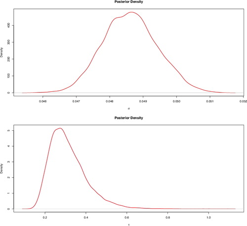
The posterior densities of σ and τ are displayed in Figure 2. The true values of the fixed effects , ICAR random effects and hyperparameters were also inside their respective 95% credible intervals.

Figure 2. Posterior densities of σ (top) and τ (bottom) for the simulation study. The true parameter values are σ = 0.05 and τ = 0.4.

Second, we perform 10,000 MCMC runs of the model with and without the data quashing strategy on simulated data. Table 1 compares computational time incurred under both scenarios. We see that the model with proposed data squashing strategy is about 3 times as efficient as model without data squashing strategy.

Table 1. Computational time comparison on simulated data.

Method	User time	System time	Elapsed time
Data quashing strategy applied	7654.6 sec	3 sec	7742.29 sec
No ata uashing trategy applied	22971.35 sec	92.08 sec	23206.64 sec

5. Analysis of SEER breast cancer survival data

We analysed the survival time for n = 26, 285 breast cancer patients of New Mexico, who were registered with SEER.For MCMC, we set M =1 and δ=0.1, then we fitted the model in Section 2 with steps in Section 3.1 and 3.2. We discarded first 10,000 samples and considered next 20,000 post-burn-in samples for inference. We left every other sample out in the post-burn-in samples. The acceptance rate of the fast Metropolis Hastings procedure was 29.21%.

The credible intervals for the model parameter are tabulated in Table 2. Our findings show that mortality rate increases with age. Overall, we find that mortality rate has decreasing linear trend over time. Futhermore, our findings show that mortality rate is higher for the African Americans compared to the white population. See Figure 3. We also find that 95% credible interval for American Indians, is (−0.141, 0.222), which means, mortality rates of the American Indians are not significantly different from the whites. Our findings are in line with other works on SEER database (DeSantis, Siegel, Bandi, & Jemal, 2011; Jatoi, Chen, Anderson, & Rosenberg, 2007; Newman et al., 2006; Roesnberg, Chia, & Plevritis, 2005). For instance, DeSantis et al. (2011) found that breast cancer death rates decreaed per year for all ages combined. The decline was larger for younger women compared to older women. Also, DeSantis et al. (2011) found that breast cancer mortality rates were higher for the African Americans whereas breast cancer mortality rates for the American Indian were comparable to the whites.

Figure 3. Posterior densities of the factor effect of black (top) and American Indian (bottom) races for SEER breast cancer New Mexico data.

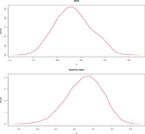
Table 2. 95% posterior credible intervals of selected parameters for the New Mexico breast cancer data.

		95% posterior credible interval
Parameter	Interpretation	Lower limit	Upper limit
β1	Patient age at diagnosis	−0.014	−0.009
β2	Calendar year of diagnosis	0.022	0.030
ζ2	Race : African American	−0.941	−0.364
ζ3	Race : Native American	−0.141	0.222
χ2	Tumor grade 2	−1.020	−0.820
χ3	Tumor grade 3	−1.869	−1.657
χ4	Tumor grade 4	−2.204	−1.751
χ3 − χ4	Difference between tumor grade 3 and 4	−0.047	0.433
K	Number of latent DP clusters	52	83
σ	AFT error s.d.	0.543	0.573
τ	DP base distribution s.d.	1.849	3.135
ση	CAR s.d.	0.225	0.509

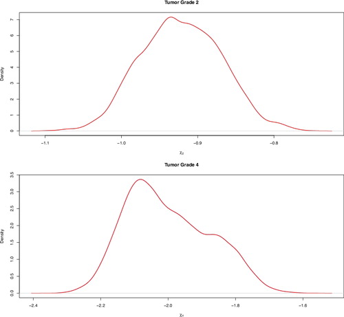
Furthermore, we find that mortality rate is higher for patients with less differentiated tumors. See Figure 4. Evidence for that is provided by the increasingly negative coefficients of tumor grade in Table 2. Our findings is in line with other peer reviewed articles (Carter, Allen, & Henson, 1989; Roesnberg et al., 2005). For instance, Roesnberg et al. (2005) found that higher grade tumor had large negative effects on survival. However, we find that the tumor effect flattens out for higher grades. We see that the 95% credible interval for (χ₃ − χ₄) is (−0.047, 0.433), which indicates that grade 3 (poorly differentiated) tumors and grade 4 (undifferentiated/anaplastic) tumors are not significantly different.

Figure 4. Posterior densities of the factor effect of tumor grade 2 at diagnosis (top) and tumor 4 at diagnosis (bottom).

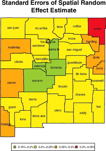
The estimates of ICAR random effects indicate that county-specific random effects are correlated with random effects of the neighbouring counties, demonstrating spatial correlation in mortality rates among counties of New Mexico. For instance, counties neighbouring Los Alamos form a cluster of counties with high spatial random effects. See Figure 5. Our finding that the mortality rates are spatially correlated concur with other peer-reviewed articles (Banerjee et al., 2015, 2003; Diva et al., 2007; Zhao et al., 2009; Zhou & Hanson, 2015). The estimates of ICAR random effects are plotted in Figure 5 with the standard errors in Figure 6.

Figure 5. Estimates of the county-specific random effects for New Mexico. The labels are the county names.

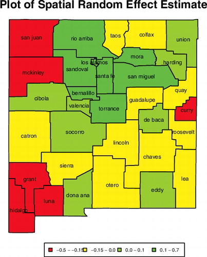
Figure 6. Standard errors of the county-specific random effects for New Mexico. The labels are the county names.

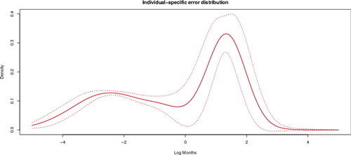
The posterior densities of several fixed effects (see Figure 4) appear to be non-normal, demonstrating the value of finite-sample approaches relative to approaches that rely on asymptotic normality of regression coefficient estimates. Figure 7 plots the estimated individual-specific error distribution F, defined as the convolution of the (discrete) realisation P of the DP with iid normal errors: (11) with * denoting convolution. Distribution F represents the residual variability in individual mortality after accounting for fixed effects and spatial variation. The gains associated with the large amount of information in massive datasets are demonstrated in Figure 7. There is strong evidence that after accounting for known indicators of disease prognosis, individual variability in breast cancer survival time is non-normal and multimodal.

Figure 7. Posterior density of the individual-specific error distribution F defined in Equation (11(11) ). See the text for the interpretation of F. The narrow lines represent margins of 2 posterior standard deviations.

We ran a nonparametric bayes version of mixed effects cox regression with independent spatial random effects (see Zhou & Hanson, 2015) on the data for comparison. See Table 3 We find that the coefficients for patient age, African Americans, American Indians, tumor grade 2, tumor grade 3 and tumor grade 4 are positive, which implies an increase in log hazard ratio with unit increase in covariates and therefore, has a negative effect on survival time. Moreover, coefficients for calendar year of diagnosis is negative, which implies a decrease in log hazard ratio and therefore has a positive effect on survival time. Furthermore, we find that coefficients for American Indians are not significant. However, we don't find that difference in tumor grade 3 and grade 4 are not significant, but we do see that tumor grade 4 effects are flattened out (see Table 3 ). Overall, we find that general results from mixed effect cox model supports our findings.

Table 3. Mixed effects cox regression for the New Mexico breast cancer data.

	95% posterior credible interval
Risk factor	Lower limit	Upper limit
Patient age at diagnosis	0.006482	0.011040
Calendar year of diagnosis	−0.038927	−0.031033
Race : African American	0.277142	0.730987
Race : Native American	−0.107270	0.267932
Tumor grade 2	0.725362	0.958409
Tumor grade 3	1.320884	1.549013
Tumor grade 4	1.125061	1.520721
Difference of Tumor grade 3 and 4	0.028292	0.195823

6. Discussion

In this paper, we proposed a semiparametric AFT model for censored outcome survival data that incorporates spatial variability. We model the spatial frailty using ICAR, which helps us capture spatial dependency in mortality rates across counties. Our model improves the flexiblity of AFT model by modeling the inter-subject variation as DP mixture. This enables our model to adapt to arbitrary features such as skewness and multimodality. The results further indicate that posterior distribution of several model parameters are non-normal and that the posterior distribution of residual individual variability is both non-normal and multimodal. Finally,we implemented a fast data squashing strategy to analyse large survival databases. This makes a strong case for using semiparametric Bayes methods for analysing large correlated survival datasets. However, the proposed model does have limitations. One drawback is that we have assumed constant variance for the spatial frailties for all the counties. This is a reasonable assumption to make when we have enough data points for every count. However, when the number of instances per county is low, it might be worth exploring CAR priors or even hierarchical priors on the variance. Furthermore, future work in this area is needed to model the temporal variation in a county's mortality.

Acknowledgments

This work was supported by the National Science Foundation under award DMS-1461948 to SG.We would also like to thank the reviewers for useful comments and suggestions that improved the presentation of the paper.

Disclosure statement

No potential conflict of interest was reported by the authors.

Additional information

Funding

National Science Foundation [grant number DMS-1461948].

References

- Antoniak, C. E. (1974). Mixtures of Dirichlet processes with applications to Bayesian nonparametric problems. Annals of Statistics, 2, 1152–1174.
- Banerjee, S., Carlin, B. P., & Gelfand, A. E. (2015). Hierarchical modeling and analysis for spatial data. (2nd ed.). Boca Raton, FL: Chapman and Hall/CRC Press.
- Banerjee, S., Wall, M. M., & Carlin, B. P. (2003). Frailty modeling for spatially correlated survival data, with application to infant mortality in Minnesota. Biostatistics, 4(1), 123–142.
- Besag, J., Mollie, A., & York, J. (1991). Bayesian image restoration, with two applications in spatial statistics. Annals of the Institute of Statistical Mathematics, 43, 1–20.
- Blackwell, D., & MacQueen, J. B. (1973). Ferguson distributions via Pólya urn schemes. The Annals of Statistics, 1, 353–355.
- Blei, D. M., & Jordan, M. I. (2005). Variational inference for Dirichlet process mixtures. Bayesian Analysis, 1, 1–23.
- Buckley, J., & James, I. (1979). Linear regression with censored data. Biometrika, 66(3), 429–436.
- Bush, C. A., & MacEachern, S. N. (1996). A semi-parametric Bayesian model for randomized block designs. Biometrika, 83, 275–285.
- Carlin, B. P., & Hodges, J. S. (1999). Hierarchical proportional hazards regression models for highly stratified data. Biometrics, 55(4), 1162–1170.
- Carter, C. L., Allen C., & Henson D. E,. (1989). Relation of tumor size, Lymph node status, and survival in 24,740 breast cancer cases. Cancer, 63, 181–187.
- Cox, D. R. (1975). Partial likelihood. Biometrika, 62, 269–276.
- DeSantis, C., Siegel, R., Bandi, P., Jemal, A. (2011). Breast cancer statistics, 2011. CA A Cancer Journal for Clinicians, 61(6), 409–18.
- Diva, U., Banerjee, S., & Dey D. K,. (2007). Modelling spatially correlated survival data for individuals with multiple cancers. Stat Modelling, 7(2), 191–213.
- DuMouchel, W., Volinsky, C., Johnson, T., Cortes, C., & Pregibon, D. (1999). Squashing flat files flatter. In Proceedings of the Fifth ACM conference on knowledge discovery and data mining (pp. 6–15).
- Escobar, M. D. (1994). Estimating normal means with a Dirichlet process prior. Journal of the American Statistical Association, 89, 268–277.
- Escobar, M. D., & West, M. (1995). Bayesian density estimation and inference using mixtures. Journal of the American Statistical Association, 90, 577–588.
- Ferguson, T. S. (1973). Estimating normal means with a Dirichlet process prior. Annals of Statistics, 1, 209–230.
- Freedman, D. (1963). On the asymptotic behavior of bayes estimates in the discrete case. Annals of Mathematical Statistics, 34, 1386–1403.
- Gelfand, A. E., & Mallick, B. K. (1995). Bayesian analysis of proportional hazards models built from monotone functions. Biometrics, 51, 843–852.
- Ghosal, S., Ghosh, J. K., & Ramamoorthi, R. V. (1999). Posterior consistency of Dirichlet mixtures in density estimation. The Annals of Statistics, 27(1), 143–158.
- Guha, S. (2010). Posterior simulation in countable mixture models for large datasets. Journal of the American Statistical Association, 105, 775–786.
- Hanson, T. E. (2006). Inference for mixtures of finite Polya tree models. Journal of the American Statistical Association, 101(476), 1548–1565.
- Hanson, T. E., Jara, A., Zhao, L. (2011). A Bayesian semiparameteric temporally-stratified proportional hazard model with spatial frailities. Bayesian Analysis, 6(4), 1–48.
- Hanson, T. E., & Johnson, W. O. (2002). Modeling regression error with a mixture of Polya trees. Journal of the American Statistical Association, 97(460), 1020–1033.
- Hanson, T. E., & Yang, M. (2007). Bayesian semiparametric proportional odds models. Biometrics, 63(1), 88–95.
- Hennerfeind, A., Brezger, A., & Fahrmeir, L. (2006). Geoadditive survival models. Journal of the American Statistical Association, 101(475), 1065–1075.
- Ibrahim, J. G., Chen, M. H., & Sinha, D. (2001). Bayesian survival analysis. New York, NY: Springer Verlag.
- Ishwaran, H., & Zarepour, M. (2002). Dirichlet prior sieves in finite normal mixtures. Statistica Sinica, 12, 941–963.
- Jatoi, I., Chen, B. E., Anderson W. F., & Rosenberg, P. S. (2007). Breast cancer mortality trends in the united states according to estrogen receptor status and age at diagnosis. Journal of Clinical Oncology, 25(13), 1683–1690.
- Kalbfleisch, J. D. (1978). Nonparametric Bayesian analysis of survival time data. Journal of the Royal Statistical Society, Series B (Methodological), 40, 214–221.
- Kay, R., & Kinnersley, N. (2002). On the use of the accelerated failure time model as an alternative to the proportional hazards model in the treatment of time to event data: A case study in influenza. Drug Information Journal, 36, 571–579.
- Kneib, T., & Fahrmeir, L. (2007). A mixed model approach for geoadditive hazard regression. Scandinavian Journal of Statistics, 34(1), 207–228.
- Komárek, A., & Lesaffre, E. (2007). Bayesian accelerated failure time model for correlated censored data with a normal mixture as an error distribution. Statistica Sinica, 17, 549–569.
- Komárek, A., & Lesaffre, E. (2008). Bayesian accelerated failure time model with multivariate doubly-interval-censored data and flexible distributional assumptions. Journal of the American Statistical Association, 103, 523–533.
- Kottas, A., & Gelfand, A. E. (2001). Bayesian semiparametric median regression modeling. Journal of the American Statistical Association, 95, 1458–1468.
- Kuo, L., & Mallick, B. (1997). Bayesian semiparametric inference for the accelerated failure-time model. Canadian Journal of Statistics, 25, 457–472.
- Li, Y., & Ryan, L. (2002). Modeling spatial survival data using semiparametric frailty models. Biometrics, 58(2), 287–297.
- MacEachern, S. N. (1994). Estimating normal means with a conjugate style Dirichlet process prior. Communications in Statistics: Simulation and Computation, 23, 727–741.
- Müller, P., Quintana, F. A., Jara, A., & Hanson, T. (2015). Bayesian nonparametric data analysis. New York, NY: Springer.
- Neal, R. M. (2000). Markov chain sampling methods for Dirichlet process mixture models. Journal of Computational and Graphical Statistics, 9, 283–297.
- Newman L. A., Griffith, K. A. Jatoi, I. Simon, M. S., Crowe, J. P., & Colditz, G. A. (2006). Meta-analysis of survival in african american and white american patients with breast cancer: Ethnicity compared with socioeconomic status. Journal of Clinical Oncology, 24(9), 1342–1349.
- Nieto-Barajas, L. E. (2013). Lévy-driven processes in Bayesian nonparametric inference. Boletín de la Sociedad Matemática Mexicana, 19, 267–279.
- Pan, C., Cai, B., Wang, L., & Lin, X. (2014). Bayesian semi-parametric model for spatial interval-censored survival data. Computational Statistics & Data Analysis, 74, 198–209.
- Pennell, M. L., & Dunson, D. B. (2007). Fitting semiparametric random effects models to large data sets. Biostatistics, 4, 821–834.
- Roesnberg, J., Chia, Y. L., & Plevritis S,. (2005). The effect of age, race, tumor size, tumor grade, and disease stage on invasive ductal breast cancer survival in the U.S SEER database. Breast Cancer Research and Treatment, 89(1), 47–54.
- Sethuraman, J. (1994). A constructive definition of Dirichlet priors. Statistica Sinica, 4, 639–650.
- Sethuraman, J., & Tiwari, R. C. (1982). Convergence of Dirichlet measures and the interpretation of their parameter. In S. S. Gupta, & J. O. Berger (Eds.), Statistical decision theory and related topics III, in two volumes (Vol. 2, pp. 305–315). New York, NY: Academic Press.
- Surveillance, Epidemiology, and End Results (SEER) Program (www.seer.cancer.gov) Limited Use Data (1973–2012). National Cancer Institute, DCCPS, Surveillance Research Program, Cancer Statistics Branch, released April 2015, based on the November 2014 submission.
- Walker, S. G., & Mallick, B. K. (1999). A Bayesian semiparametric accelerated failure time model. Biometrics, 55(2), 477–483.
- West, M., Müller, P., & Escobar, M. D. (1994). Hierarchical priors and mixture models, with application in regression and density estimation. In A. F. M. Smith & P. Freeman (Eds.), Aspects of uncertainty: A tribute to D. V. Lindley (pp. 363–368). New York, NY: Wiley.
- Zhao, L., Hanson, T. E., & Carlin, B. P. (2009). Mixtures of Polya trees for flexible spatial frailty survival modelling. Biometrika, 96(2), 263–276.
- Zhou, H., & Hanson, T. (2015). Bayesian spatial survival models. In R. Mitra & P. Müller (Eds.), Nonparametric Bayesian inference in biostatistics. Frontiers in probability and the statistical sciences. Springer.
- Zhou, H., & Hanson, T. (2017). A unified framework for fitting Bayesian semiparametric models to arbitrarily censored survival data, including spatially-referenced data. Journal of the American Statistical Association, ( to appear).