Factor analysis of correlation matrices when the number of random variables exceeds the sample size

ABSTRACT

Factor analysis which studies correlation matrices is an effective means of data reduction whose inference on the correlation matrix typically requires the number of random variables, p, to be relatively small and the sample size, n, to be approaching infinity. In contemporary data collection for biomedical studies, disease surveillance and genetics, p > n limits the use of existing factor analysis methods to study the correlation matrix. The motivation for the research here comes from studying the correlation matrix of log annual cancer mortality rate change for p = 59 cancer types from 1969 to 2008 (n = 39) in the U.S.A. We formalise a test statistic to perform inference on the structure of the correlation matrix when p > n. We develop an approach based on group sequential theory to estimate the number of relevant factors to be extracted. To facilitate interpretation of the extracted factors, we propose a BIC (Bayesian Information Criterion)-type criterion to produce a sparse factor loading representation. The proposed methodology outperforms competing ad hoc methodologies in simulation analyses, and identifies three significant underlying factors responsible for the observed correlation between cancer mortality rate changes.

KEYWORDS:

• Alpha spending function
• BIC
• cancer surveillance
• eigenvalues
• sparse factor loadings

1. Introduction

Due to its flexibility in characterising multivariate data, high-dimensional factor analysis is becoming popular in many scientific disciplines including genetic (Zhou, Wang, Wang, Zhu, & Song, 2017), biomedical (Shimizu et al., 2016) and economic studies (Fan, Lv, & Qi, 2011). The objectives of exploratory factor analysis are twofold: (1) identify the number of factors that influence a set of random variables; (2) measure the strength of the relationship between the extracted factors and each random variable.

In many studies where the random variables of interest are highly variable (e.g., cancer mortality rates), it is common to standardise the random variables and analyse the correlation matrix. Standardisation ensures that results from factor analysis will not be driven by random variables with large variances, which is a challenge when performing factor analysis on covariance matrices. Additionally, in the cases where the number of random variables exceeds the sample size, a couple of statistical challenges arise in the analysis of correlation matrices via factor models. First, existing inference methods rely on the number of random variables, p, to be relatively small and fixed, and the sample size, n, to be approaching infinity (Anderson, 1963; Johnson & Wichern, 1998). Another complication is that factor analysis is not invariant to change on the scale of variables. Methods that infer structure from covariance matrices (Bickel & Levina, 2008; Carvalho et al., 2008; Fan, Fan, & Lv, 2008; Ghosh & Dunson, 2009; Huang, Liu, Pourahmadi, & Liu, 2006; Patterson, Price, & Reich, 2006; West, 2003; Wong, Carter, & Kohn, 2003) will not always perform similarly on correlation matrices. There appears to be a lack of methodology for performing inference on correlation matrices using factor analysis when p > n. Furthermore, traditional methods for estimating the number of factors to be extracted and their interpretation are insufficient and need further development for correlation matrices when p > n.

We make several contributions with this paper. First, we formalise a test statistic to perform inference of the structure of the correlation matrix using the limiting distribution of eigenvalues. This test statistic from Johnstone (2001) but was not delineated as fully as we do in this paper. Second, we extend the work of Johnstone (2001) to identify the true number of underlying factors present in a factor model, while controlling the type I error. Finally, we propose a BIC (Bayesian Information Criterion)-type criterion to produce sparse factor loadings to ease interpretation of extracted factors.

The format of this paper is as follows. In Section 2, we present a test for inference on the structure of the population correlation matrix, which we term the Tracy–Widom test. In Section 3, we develop a sequential-rescaling procedure to test for the number of significant factors in a given factor model. Section 4 describes a sparse factor model that aids in interpreting the factors detected from the proposed test. Section 5 presents some designed simulation studies based on the proposed methodology. Section 6 applies the developed methodology to study the correlation matrix of cancer mortality ARC data, followed by our concluding remarks in Section 7.

2. Methods

2.1. Factor model formulation

Consider a random vector X = (X₁,… , X_p)^T where each component X_j follows a standard normal distribution. Because different cancers have varying degrees of volatility, normalisation will ensure that the analysis will not be dominated by a few cancer types. The primary aim of this project is to study the correlation matrix of X.

A factor model postulates that X is linearly dependent on a few underlying, but unobservable, random quantities F₁,… , F_m called common factors and p additional sources of variation ε₁,… , ε_p called white noise or specific factors, such that (1) where is a vector of m common factors, is a p × m matrix of factor loadings with ℓ_l = (ℓ_l1,… , ℓ_lp)^T for l = 1,… , m and is an identity matrix of dimension m. We denote the residual as where is a p × p diagonal matrix with the lth diagonal element being ψ_l = 1 − ℓ²_1l − ⋅⋅⋅ − ℓ²_ml to ensure that Var(X_j) = 1.

If we assume that and are independent in Equation (1(1) ), then it follows that the correlation matrix for X is . Using an eigenvalue decomposition, with m orthonormal eigenvectors for l = 1,… , m such that λ₁ ≥ λ₂ ≥ · · · ≥ λ_m ≥ 0 and , which equals 1 if l = k and 0 otherwise. Hence, and results in (2) where λ₁, λ₂,… , λ_m correspond to the m largest eigenvalues of .

2.2. Testing complete independence of the correlation matrix

One of the first objectives of studying the correlation matrix of a set of random variables is to determine if factor analysis is a reasonable method of analysis. This is equivalent to performing inference on the structure of the correlation matrix with test of versus the alternative . We base our test for on the largest eigenvalue of the sample correlation matrix of X. A result of random matrix theory (RMT) suggests that we can build a theoretical distribution for the largest eigenvalue of random matrices under the null hypothesis of complete independence (Johnstone, 2001). A test of complete independence about the p random variables compares the observed sample eigenvalue to the theoretical distribution of λ₁ under RMT prediction. This test will reveal one of two possibilities: the first being that will be determined to not significantly differentiate from RMT prediction. This suggests that cannot be rejected and therefore that factor analysis will not prove to be useful because specific noise factors play a more dominant role in the observed correlation than common underlying factors. The second possibility for a test of the largest eigenvalue is that it will determine to significantly deviate from RMT prediction (i.e., is rejected in favour of the alternative). This scenario suggests that one (or possibly more) underlying factor(s) could be responsible for the observed correlation between the random variables.

To proceed, we describe the test statistic for testing . Suppose that data matrix has entries that are independent and identically distributed as standard normal. Let denote the sample eigenvalues of a Wishart Matrix, . We can test the significance of , the largest eigenvalue of , with test statistic (3) where and

Johnstone (2001) has shown that under H₀, and n, p → ∞ such that n/p → γ for γ some constant and the test statistic , where W₁ is called the Tracy–Widom distribution (Tracy & Widom, 2000). We term (3(3) ) the Tracy–Widom test and will reject the null hypothesis of when T_np > W_{1, 1 − α} where W_{1, 1 − α} is the (1 − α) × 100 percentile of the Tracy–Widom distribution. One of the strengths of this test is that it can be applied in the classical setting where n > p as well as in high-dimensional settings where p > n.

2.3. Correlation correction of Tracy–Widom test

A technical note suggests that the Tracy–Widom test applies to the study of covariance matrices and does not directly apply to correlation matrices, which is problematic for distribution theory (Anderson, 1963). To be able to apply the Tracy–Widom test to study correlation matrices, we expand on the procedure that was briefly mentioned in Johnstone (2001) but has not been fully studied. To this end, suppose we draw n i.i.d. row vector samples from to produce data matrix . Under the null hypothesis, the column vectors are i.i.d on the unit sphere S^{n − 1}. As a result, we can multiply each by an independent chi-distributed length to synthesise a Gaussian matrix, call it such that where and ψ²_j ∼ χ²_{(n − 1)}. We can then construct a sample pseudo-covariance matrix which approximately follows a Wishart distribution with n − 1 degrees of freedom. Under the null, this data augmentation allows us to apply the Tracy–Widom test on the largest eigenvalue of to test .

3. Identifying additional factors

If is rejected, then at least one latent factor is useful in describing the observed correlation among the p random variables. One of the most crucial steps of factor analysis is to estimate the true number of underlying factors, m, as misspecification of the number of factors retained can lead to poor factor-loading pattern reproduction and interpretation (Hayton, Allen, & Scarpello, 2004). Furthermore, estimation of the number of factors can affect the factor model results more than other decisions, such as the factor rotation method used (Zwick & Velicer, 1986). In this section, we extend the work of Johnstone (2001) to identify the number of relevant factors to be used in a factor model.

Previous work on estimating the number of factors have focused on factor analysis for covariance matrices (Bai, 2003; Bai & Ng, 2002; Leek, 2011; Onatski, 2009). Johnstone (2001) and Baik and Silverstein (2006) have considered the asymptotic behaviour of , the (r + 1)th largest eigenvalue of a covariance matrix, when the true population covariance follows a spiked model with , where τ₁ ≥ · · · ≥ τ_r > 1. As factor analysis is not invariant to changes in the scale of the variables, it is often recommended that factor analysis be performed for standardised variables. Standardisation converts a covariance matrix problem into a correlation problem and it is unclear how these methods would be applied to the study of sample correlation matrices.

Common ad hoc methods of determining the number factors to extract from correlation matrices include the scree plots, Guttman–Kaiser criterion and parallel analysis. The number of extracted factors based on the scree plot is highly subjective as the estimate is visually selected as point that resembles an elbow. The Guttman–Kaiser criterion (Guttman, 1954; Kaiser, 1960) selects the number of factors to be equal to the number of sample eigenvalues of the correlation matrix that are greater than one. Parallel analysis (Horn, 1965) is a simulation-based approach that compares the eigenvalues of the sample correlation matrix to eigenvalues from a matrix of random values of the same dimensionality. The estimated number of factors retained are the number of observed sample eigenvalues greater than the 95th percentile of the distribution of eigenvalues derived from the random data.

3.1. Sequential-rescaling testing procedure

We propose to view the testing procedure of extracting relevant underlying factors as a sequential procedure. Given that the Tracy–Widom test is used to test the largest eigenvalue, we propose a sequential method that removes the effect of the first factor (if significant) and produces a new data matrix from which we can construct a new correlation matrix and apply once again the Tracy–Widom test on the new largest eigenvalue. In general, we will test for the significance of λ_k only after verifying that λ_{k − 1} are significantly different than RMT prediction and after eliminating the effect of the first k − 1 factors. We remove the effect of the first k − 1 factors because of the phenomenon where the largest eigenvalue has the potential to pull other sample eigenvalues away from unity. The resulting procedure is termed a sequential-rescaling procedure. The advantage of the procedure that follows is that it controls the type I error through the use of an alpha spending function, and it is not a conservative technique based on what has been proposed in Patterson et al. (2006).

Suppose we have declared the first k − 1 eigenvalues to be significantly different than RMT prediction. The following procedure tests the subsequent eigenvalue λ_k. The procedure assumes the Tracy–Widom test has already identified λ₁, λ₂,… , λ_{k − 1} to be significant. Associated with eigenvalue λ_ℓ is its corresponding eigenvector . We proceed to test λ_k through the following two-step procedure:

• Construct a data matrix such that (4) where is the rescaling diagonal matrix with its ith diagonal element being D_{k − 1, ii} = 1 − λ_{k − 1}e²_{k − 1, i}. The rescaling matrix, will assure the desirable property that var. Note that we have removed the effect of the first k − 1 factors in Equation (4(4) ) through the term.

• It can be shown that the sample correlation matrix for the rescaled , on which we will test the significance of λ_k using the Tracy–Widom test proposed in Equation (3(3) ) is (5) We perform this two-step procedure applying the Tracy–Widom test on each subsequent eigenvalue until an eigenvalue is no longer significant.

We note that caution should be taken when testing subsequent sample eigenvalues. To circumvent the multiple testing issues that are present in this procedure, we apply methodology from the group sequential analysis literature to control the type I error. Lan and DeMets (1983) proposed an alpha spending technique in which the nominal significance level needed to reject the null hypothesis at each analysis is less than α and increases as the study progresses. If an overall type I error (α) is desired, we propose to use the following alpha spending function: (6) where α*(k) is the significance level for the kth hypothesis test. This is opposed to Lan and DeMets (1983), as alpha spending function (6(6) ) does not depend on the overall number of tests being conducted. Therefore, one need not specify the maximum number of eigenvalues being tested, which is ideal for unsupervised learning.

We define type I error as the probability of incorrectly choosing a model that has extracted more factors than the true model. Compared to Lan and DeMets (1983) who suggest that the alpha spending function should be non-decreasing, our spending function is non-increasing (α*(1) > α*(2) > · · · > α*(K)); because finding a parsimonious model is preferred, we need strong evidence for choosing a more complicated model with more significant eigenvalues over a simpler one. We have shown in supplementary material that the overall type I error rate using the proposed spending function (6(6) ) will not exceed α.

4. Interpretation of factors

After an estimation is made for the number of factors to be used, the next objective in factor analysis is to provide an interpretation for each underlying factor. In principle, the factor loadings provide the basis for interpreting the factors underlying the data. The size and direction of the extracted factor loadings denote the strength and direction of the correlation between the random variables and the extracted factors. Traditionally, the task of interpreting factors has been subjective and unsatisfactory.

Because the original factor loadings may not be easily interpretable, it has become common to rotate the loadings (e.g., varimax, oblique, etc.) to increase or decrease the size of factor loadings to ease of interpretation. Unfortunately, regardless of the factor rotation used, it is rare for factor loadings to be set exactly to zero which would ease in the interpretation of the underlying factor.

With the recent developments of regularised regression in mind, we propose to implement a regularisation technique to detect a set of sparse factor loadings for easier interpretation of identified factors. The resulting sparse factor loading vector sets the loadings of negligible random variables to zero, assuring that they will not contribute to the interpretation of the underlying factor, making the interpretation of the factors more straightforward. Additionally, because negligible random variables are removed, the variance explained by the sparse factor loadings will not suffer much from their removal.

Eigenvalue decomposition (2(2) ) provides the factoring of the correlation matrix of . The factor loading matrix is given by where are the eigenvalue–eigenvector pairs of . Producing sparse factor loadings is equivalent to setting components of to zero. It can be shown that apart from the scale value , the factor loading column are the coefficients of the principal components of the population. This observation allows us to implement well-studied sparse principal components methods to produce sparse factor loadings.

We propose to regularise for l = 1,… , m using the sparse principal components analysis (SPCA) method proposed by Zou, Hastie, and Tibshirani (2006). SPCA essentially takes the problem of setting PCA loadings to zero and transforms it into a regression-type problem that uses an elastic net regularisation technique to detect sparse loadings even when p > n. Details of SPCA methodology can be found in Zou et al. (2006), but we provide a brief description in the following.

4.1. SPCA for sparse factor loadings

We consider the problem of producing sparse factor loadings for the m estimated factors. Let , and be the n × p data matrix as before and denote the ith row vector of . The problem of producing sparse factor loadings can be transformed into the following regression-type criterion with an elastic net penalty: (7) for any γ > 0. The last term in Equation (7(7) ) uses the L₁ penalty to produce sparse factor loadings because the estimated sparse factor loadings, defined as for l = 1,… , m, are a function of the sparse β_l vector.

4.2. Selection of tuning parameter

The optimisation problem in Equation (7(7) ) contains two tuning parameters that must be selected. The first tuning parameter, γ, is the same for all the m factors. It has been shown (Zou et al., 2006) that when p > n, a positive γ is required to produce exact loadings when the second tuning parameter is set to zero. The tuning parameter γ has been studied and is well understood. Empirical evidence has shown that for the case when n > p, γ can be set to zero. When p > n, γ can be set to a small positive number to overcome collinearity between the columns of .

The second tuning parameter γ_{1, l} is a factor-specific tuning parameter and requires more development. Zou et al. (2006) did not provide clear guidance on selecting γ_{1, j}, other than choosing γ_{1, j} such that it provides a good compromise between explained variance and sparsity. Other methods exist for selecting the tuning parameters, such as cross validation (Shen & Huang, 2008) which could be computationally extensive and requires a large sample size. We add to the current literature on producing sparse factor loadings by proposing a BIC-type criterion for selecting the factor specific tuning parameters (γ_{1, 1},… , γ_{1, m}).

For a fixed γ, we propose to use the following BIC-type criterion for selection of tuning parameters (γ_{1, 1},… , γ_{1, m}): (8) where , is the factor loading matrix and where . We define the degrees of freedom, , to be the number of non-zero loadings in the loading matrix . Zou, Hastie, and Tibshirani (2007) showed that the number of of non-zero coefficients in lasso regression provides an unbiased estimate for the degrees of freedom and suggests that BIC can be used to determine the optimal number of nonzero factor loadings.

5. Analysis of simulated data

To assess the performance of the proposed method, we simulate data from factor models where the p observable random variables are constructed from zero, one, two or three underlying factors. The zero factor model is given by X_j = ε_j where ε_j ∼ N(0, 1) for j = 1,… , p. The one factor model is given by where U₁ ∼ Unif(0, 1) and F₁ ∼ N(0, 1). The two factor model is simulated from where U₂ ∼ Unif(0.5, 1.5) and . Finally, the three-factor model is simulated from the following model: where U₃ ∼ Unif(1, 1.5) and .

We consider configurations of the data by taking n samples from each of the factor models and we vary p to be less than, equal to or more than n. The following parameter configurations are considered: (p = 100, n = 500), (p = 500, n = 500), (p = 500, n = 100). We also consider the special case when p = 59, n = 39, which is the number of distinct cancer types and the sample size of the SEER cancer mortality data. In this special case, the number of random variables loading on F₁ is 25, the number of random variables loading on F₂ is 15 and 10 on F₃.

5.1. Simulation results for estimating the number of factors

In this section, we use the simulated data-sets to demonstrate the behaviour of the sequential-rescaling procedure when used to estimate the number of factors in a model with zero, one, two or three underlying factors. We compare the proposed procedure to the Guttman–Kaiser criterion and parallel analysis.

We present simulation results in Table 1 for 1500 simulated data-sets derived from zero-, one-, two- or three-factor models. The results in Table 1 shows that the proposed method performs well, and in almost all cases outperforms the Guttman–Kaiser criterion and parallel analysis. The Guttman–Kaiser criterion consistently overestimates the number of factors to be retained, compared to other methods (even when n > p). We note that when p is vastly larger than n, the Guttman–Kaiser criterion always estimates the number of factors to be the rank of .

Table 1. Simulation results based on 1500 simulated data-sets for selecting the true number of factors comparing Guttman criterion (Gu), parallel analysis (Pa) and the proposed methodology (Pr). Presented is the discrete probability of the estimated number of factors and its corresponding mean and standard deviation for one-, two- and three-factor models. The number of random variables (p) and sample size (n) are varied.

		Zero-factor			One-factor			Two-factor			Three-factor
(p, n)		Gu	Pa	Pr	Gu	Pa	Pr	Gu	Pa	Pr	Gu	Pa	Pr
(100, 500)	0	0.00	0.95	0.98	0.00	0.00	0.00	0.00	0.00	0.00	0.00	0.00	0.00
	1	0.00	0.04	0.02	0.00	0.92	0.98	0.00	0.00	0.01	0.00	0.00	0.00
	2	0.00	0.01	0.00	0.00	0.08	0.02	0.00	0.99	0.97	0.00	0.00	0.00
	3	0.00	0.00	0.00	0.00	0.00	0.00	0.00	0.01	0.03	0.00	1.00	0.97
	4+	1.00	0.00	0.00	1.00	0.00	0.00	1.00	0.00	0.00	1.00	0.00	0.03
		45.32	0.07	0.02	41.68	1.09	1.02	35.81	2.01	2.03	25.26	3.00	3.03
		0.73	0.34	0.14	0.73	0.33	0.15	0.74	0.10	0.17	0.75	0.00	0.17
(500, 500)	0	0.00	0.95	0.98	0.00	0.00	0.00	0.00	0.00	0.00	0.00	0.00	0.00
	1	0.00	0.03	0.02	0.00	0.74	0.98	0.00	0.00	0.00	0.00	0.00	0.00
	2	0.00	0.01	0.00	0.00	0.18	0.02	0.00	0.68	0.99	0.00	0.00	0.00
	3	0.00	0.01	0.00	0.00	0.05	0.00	0.00	0.22	0.01	0.00	0.88	0.99
	4+	1.00	0.00	0.00	1.00	0.03	0.00	1.00	0.10	0.00	1.00	0.12	0.01
		195.65	0.07	0.02	194.31	1.39	1.02	191.51	2.45	2.01	185.54	3.14	3.01
		0.85	0.38	0.15	0.85	0.82	0.13	0.84	0.80	0.10	0.84	0.38	0.06
(500, 100)	0	0.00	0.97	0.97	0.00	0.04	0.01	0.00	0.00	0.00	0.00	0.00	0.00
	1	0.00	0.03	0.03	0.00	0.47	0.98	0.00	0.00	0.01	0.00	0.00	0.00
	2	0.00	0.00	0.00	0.00	0.19	0.01	0.00	0.02	0.98	0.00	0.00	0.01
	3	0.00	0.00	0.00	0.00	0.05	0.00	0.00	0.01	0.01	0.00	0.00	0.98
	4+	1.00	0.00	0.00	1.00	0.25	0.00	1.00	0.97	0.00	1.00	1.00	0.01
		99.00	0.03	0.03	99.00	21.94	1.00	99.00	382.91	2.00	99.00	445.02	2.99
		0.00	0.18	0.16	0.00	88.39	0.14	0.00	126.46	0.15	0.00	5.50	0.13
(59, 39)	0	0.00	0.96	0.97	0.00	0.01	0.02	0.00	0.00	0.00	0.00	0.00	0.00
	1	0.00	0.03	0.03	0.00	0.85	0.96	0.00	0.00	0.03	0.00	0.00	0.00
	2	0.00	0.01	0.00	0.00	0.11	0.02	0.00	0.91	0.96	0.00	0.00	0.04
	3	0.00	0.00	0.00	0.00	0.03	0.00	0.00	0.08	0.01	0.00	0.97	0.96
	4+	1.00	0.00	0.00	1.00	0.00	0.00	1.00	0.01	0.00	0.00	0.03	0.00
		21.55	0.05	0.03	20.76	1.17	1.00	19.21	2.09	1.98	17.77	3.03	2.97
		0.67	0.26	0.18	0.70	0.49	0.19	0.77	0.33	0.21	0.80	0.18	0.21

The parallel analysis method of estimating the number of factors is relatively accurate across the range of factor models when n > p. When p becomes comparable to n, the parallel analysis estimator overestimates m compared to the proposed methodology. As p becomes significantly larger than n, the parallel analysis estimator breaks down and significantly overestimates m.

5.2. Simulation results of BIC criterion

For each of the simulated data-sets, there are numerous random variables that have zero loadings on the underlying factors. We perform SPCA on each of the simulated extracted factor loadings to obtain vectors of factor loadings with zero loadings that can help in interpreting the underlying factors. We choose the factor-specific tuning parameters (γ_{1, 1},… , γ_{1, m}) based on the BIC criterion described in Section 4.2. We consider 200 simulated data-sets for one-, two- and three-factors models with varying (p, n) as described earlier.

We present the estimated number of non-zero factor loadings, the false positive rate and false negative rate for each factor based on sparse PCA using the proposed BIC criterion in Table 2. Across all factor models, the BIC tuning parameter selection method selects the true non-zero loadings with good consistency when n is large and when n is larger or comparable to p. When p > n, the BIC tends to select larger models for factor 2 and factor 3 and the false positive rate and false negative rate are no longer negligible.

Table 2. Simulation results based on 200 simulated data-sets for the proposed BIC-type criterion tuning parameter selection. The |ℓ_m| denotes the true number of random variables that load on each corresponding factor and denotes the mean number of non-zero factor loadings for each factor across the simulated data-sets. FP and FN denote the false positive rate and false negative rate, respectively. The number of random variables (p) and sample size (n) are varied.

		One-factor	Two-factors		Three-factors
(p, n)		F1	F1	F2	F1	F2	F3
(100, 500)	|ℓm|	30.00	30.00	20.00	30.00	20.00	25.00
		30.10	29.96	20.00	30.01	20.06	25.76
	FP	0.001	0.000	0.000	0.000	0.001	0.010
	FN	0.000	0.001	0.000	0.000	0.000	0.000
(500, 500)	|ℓm|	30.00	30.00	20.00	30.00	20.00	25.00
		30.02	28.61	20.00	30.00	20.03	25.75
	FP	0.000	0.000	0.000	0.000	0.000	0.002
	FN	0.000	0.046	0.000	0.000	0.000	0.000
(500, 100)	|ℓm|	30.00	30.00	20.00	30.00	20.00	25.00
		31.05	33.66	32.40	31.64	29.53	31.77
	FP	0.008	0.012	0.026	0.009	0.020	0.014
	FN	0.085	0.065	0.000	0.083	0.000	0.000
(59, 39)	|ℓm|	25.00	25.00	15.00	25.00	15.00	10.00
		27.94	23.63	24.36	23.41	22.63	20.00
	FP	0.177	0.122	0.228	0.115	0.310	0.289
	FN	0.123	0.221	0.044	0.220	0.402	0.415

6. Data analysis

The motivation for the proposed statistical methodology is derived from work on identifying change patterns in cancer mortality trends. Cancer mortality data for the United States come from the National Cancer Institute's Surveillance, Epidemiology and End Results (SEER) Program. We analyse age-adjusted cancer mortality change patterns separately for males and females. For the sake of brevity and to avoid redundancy, we only present the results for males.

In the study of cancer mortality change pattern trends, it is common to use the log transformed annual rate change (ARC) instead of the actual mortality rate. The ARC of cancer type j in year i denoted by ARC_ij is defined as ARC_ij = log r_ij − log r_{i − 1, j}, where r_ij denotes the cancer mortality rate of cancer type j in year i, and the log transformation is applied to normalise the data and the difference to construct independent components (Kim, Fay, Feuer, & Midthune, 2000). Because the different cancer types have varying levels of volatility, we will centre and standardise ARC_ij such that it has mean 0 and variance 1. We denote the standardised rate change as X_ij. We obtain an estimate of the correlation matrix, where is the data matrix with X_ij as its (i, j)th entry. Cancer mortality rates were obtained for p = 59 distinct male cancer types over n = 39 years (1969–2008).

6.1. Application of proposed methodology to SEER data

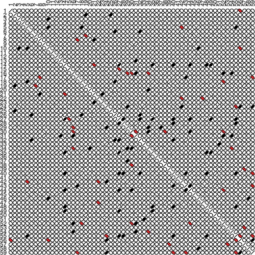
To visualise the correlation matrix of cancer ARC, we construct a correlation matrix using ellipse-shared glyphs for each entry in Figure 1. Overall, Figure 1 displays how the correlation matrix is dominated by low correlations between the cancer types. It is feasible that the population correlation matrix of ARC could be equal to the identity matrix and that the few moderate observed correlations are simply noisy estimates.

Figure 1. Visualisation of the standardised log-annual cancer mortality rate change correlation matrix of the 59 unique male cancer types. Ellipse-shared glyphs for each entry represent the level curve of a bivariate normal density with the matching correlation. Darker Ellipses denote a positive correlation greater than 0.4 and lighter ellipses denote a negative correlation of more than −0.4. Ellipses with no color denote correlation between −0.4 and 0.4. The cancer type can be matched to the number on the figure and in Table 4.

We begin our investigation of the correlation matrix of ARC by testing the null hypothesis versus the alternative . To test this hypothesis, we study the largest eigenvalue of which was estimated to be 7.12. After performing the correlation correction of the Tracy–Widom test described in Section 2.3, the estimated largest eigenvalue of the pseudo-covariance matrix is 268.90. Applying the Tracy–Widom test on this value, we calculate the test statistic T_np = 8.63 where and . Compared to the Tracy–Widom distribution of order 1, the test statistic results in a p value <0.0001. We reject the null hypothesis of complete independence in ARC between cancer types which suggests that at least one factor is sufficient to describe the observed correlation among the cancer types.

Next, we determine the number of factors to be used in the analysis using the sequential rescaling procedure described in Section 3.1 and present those results in Table 3. Table 3 suggests that three underlying factors are important in characterising the correlation matrix of cancer mortality ARC.

Table 3. Sequential-rescaling procedure: largest four estimated eigenvalues of the pseudo-covariance matrix () are denoted in the second column. The p value for the corresponding Tracy–Widom test and alpha spending function, α*(k), are in the third and fourth column, respectively. The last column denotes the decision to retain or not retain the factor.

Factor		p value	α*(k)	Decision
1	268.90	<0.0001	0.0250	Retain
2	234.42	<0.0001	0.0125	Retain
3	219.46	0.0003	0.0063	Retain
4	207.17	0.0033	0.0031	Do not retain

Next, for the three extracted factors we performed sparse principle components analysis described in Section 4 to regularise the factor loadings. Only cancer types with meaningful associations to each underlying factor will have a non-zero factor loading, and we consider these to be important for the interpretation of the factors. We set γ = 1.0 × 10⁴ in our SPCA analysis because the number of cancer types exceeded the number of data points available. To determine the degree of sparsity for each factor, we selected (γ_{1, 1}, γ_{1, 2}, γ_{1, 3}) to be the values that minimised the BIC criterion in Equation (8(8) ).

We present in Table 4, the 59 unique cancer types and their corresponding sparse factor loadings for the extracted factors. Of all the 59 cancers, 28 cancer types had zero loadings on all three factors. We note that lung and bronchus, prostate and colon cancer sites load heavily on the first factor but has exactly zero loadings for factors 2 and 3. Factor 1 might provide more support to the hypothesis that, as for colorectal cancer, early detection through screening and advances in treatment for prostate cancer are important factors that underlie the change in mortality rate. Factor 2 appears to contrast soft tissue cancers and leukemia, however, it is not clearly evident what is driving to their observed correlation. The interpretation of factor 3 appears to be highly related to miscellaneous cancer types (miscellaneous malignant cancer, other myeloid/monocytic leukemia, other digestive organs, etc.). Figure A1 provides additional information on each factor and their ARC change over time.

Table 4. Specific male cancer types and their corresponding sparse factor loadings. Sparse loadings are estimated by SPCA.

#	Cancer type	Factor 1	Factor 2	Factor 3
1	Lip
2	Tongue
3	Salivary gland			−0.10
4	Floor of mouth
5	Gum and other mouth
6	Nasopharynx
7	Tonsil
8	Oropharynx
9	Hypopharynx		0.01
10	Other oral cavity and pharynx			−0.04
11	Esophagus
12	Stomach
13	Small intestine
14	Colon excluding rectum	−0.14
15	Rectum and rectosigmoid junction	0.02
16	Anus, anal canal and anorectum		0.22
17	Liver			−0.11
18	Intrahepatic bile duct	−0.04
19	Gallbladder
20	Other biliary
21	Pancreas	0.04
22	Retroperitoneum
23	Peritoneum, omentum and mesentery
24	Other digestive organs			0.30
25	Nose, nasal cavity and middle ear
26	Larynx	−0.01
27	Lung and bronchus	−0.16
28	Pleura	−0.02
29	Trachea, mediastinum and other respiratory organs
30	Bones and joints		−0.24
31	Soft tissue including heart		0.18
32	Melanoma of the skin	−0.05		−0.05
33	Other non-epithelial skin			0.05
34	Breast		−0.14
35	Prostate	−0.12
36	Testis
37	Penis
38	Other male genital organs
39	Urinary bladder
40	Kidney and renal pelvis	−0.06		−0.08
41	Ureter
42	Other urinary organs			0.08
43	Eye and orbit			−0.13
44	Brain and other nervous system	−0.05	−0.05
45	Thyroid
46	Other endocrine including thymus
47	Hodgkin lymphoma
48	Non-hodgkin lymphoma	−0.08
49	Myeloma	−0.10
50	Acute lymphocytic leukemia		−0.03
51	Chronic lymphocytic leukemia
52	Other lymphocytic leukemia		0.14
53	Acute myeloid leukemia
54	Acute monocytic leukemia		0.10
55	Chronic myeloid leukemia	−0.05		−0.12
56	Other myeloid/monocytic leukemia			0.24
57	Other acute leukemia
58	Aleukemic, subleukemic and NOS
59	Miscellaneous malignant cancer			0.34

7. Discussion

We have described a methodology based on RMT that uses factor analysis to make inference on correlation matrices for settings where p > n. The methods described herein are applicable to a wide range of data, because it can be applied to cases where p > n as well as to traditional cases where n > p. We observed that current methods for selecting the number of factors (Guttman–Kaiser criterion and parallel analysis) do not perform well when p > n. Thus, we developed a sequential-rescaling procedure to determine the number of significant factors in a factor model using the Tracy–Widom test. This procedure is based on group sequential theory to control for the overall type I error. We described a practical approach to interpret the significant factor loadings using SPCA and a novel BIC-type criterion which regularises the noisy estimates of the factor loadings. Simulation studies demonstrate great performance for the proposed methodology in selecting the number of factors to be extracted and for identifying the important random variables that load on the underlying factors.

A number of open problems present themselves. The methods herein were constructed under the normality assumption. It is unclear how to determine complete randomness against any deviation from normality. For future work, it would be ideal to study the robustness of this methodology and the Tracy–Widom test against different distributional assumptions. Another limitation is that we have not explored any methods that test whether the change patterns of any two specific cancer types are correlated over time. Factor analysis identifies groups of cancers that are linearly dependent upon a few unobservable latent random variables, but cannot make specific statements about pairwise correlations. Identifying specific pairs of cancers that share similar change patterns could be extremely useful for cancer researchers. One avenue to explore related to the identification of significant pairwise change patterns would be to regularise the elements of the correlations themselves, which have been extensively studied for covariance matrices (Cai & Liu, 2011; Fan, Liao, & Liu, 2016; Rothman, Levina, & Zhu, 2009). Finally, although our focus was on the study of the correlation matrix when p > n, future studies should compare the performance of the Tracy–Widom test and sequential-rescaling procedure on covariance matrices to compare the performance and generalisability of these methods.

Acknowledgments

The authors thank Armin Schwartzman for his insightful comments and Amanda Delzer Hill for her editing work that greatly improved the manuscript.

Disclosure statement

The authors have no conflict of interests to declare.

Additional information

Funding

This work was supported by National Institutes of Health Grants [grant number RO1 CA95747], [grant number P01CA134294-01002].

Notes on contributors

Miguel Marino

Miguel Marino is an assistant professor of biostatistics in the Department of Family Medicine at Oregon Health & Science University, with a joint appointment in the School of Public Health.

Yi Li

Yi Li is professor of biostatistics and director of the Kidney Epidemiology and Cost Center at the University of Michigan.

Appendix

In this section, we show that the proposed alpha spending function to test the number of significant factors will not exceed α, by calculating three probabilities.

(1)	Probability that a model with one or more factors is chosen given a true zero-factor model. Let Lm be the event that the true model has m significant factors and the estimated number of factors. Then it follows that
(2)	Probability that a model is selected with k factors given a true zero-factor model for any k ≥ 1. Because it follows that where the last equality follows as the result of αk < α as α ∈ (0, 1). Finally, as , we get the result that
(3)	Probability that a model is selected with more than k factors given a true factor model with k factors.

Thus, the type I error does not exceed alpha in any of the settings.

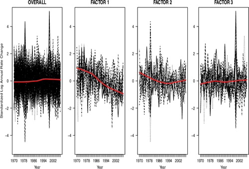
In Figure A1, we plot the cancer mortality standardised log ARC over time for for all 59 cancer types and also three separate plots for the cancer types that have non-zero loadings for each factor. To visualise the pattern over time, we fit a Lowess smoothing line across time. Overall, when we consider the change patterns of ARC for all 59 cancer types simultaneously, we do not observe much change in ARC over time. The factor analysis performed identifies three distinct cancer mortality patterns of ARC over time. Factor 1 is a collection of cancer types (primarily influenced by colon, prostate and lung cancers) that have exhibited a decrease in ARC cancer mortality across time. The cancer types in factor 2 have decreasing ARC that levels off after the year 1990. Finally, factor 3 (miscellaneous) cancer types show no change in ARC over time.

Figure A1. Line plots of standardised log annual cancer mortality rate change over time. Left panel includes all cancer types and the last three panels plot the standardised log ARC for the cancer types that have non-zero loadings on factors 1, 2 and 3, respectively. The solid thick gray line denotes Lowess smoothing curves.

References

- Anderson, T. (1963). Asymptotic theory for principal component analysis. The Annals of Mathematical Statistics, 34(1), 122–148.
- Bai, J. (2003). Inferential theory for factor models of large dimensions. Econometrica, 71(1), 135–171.
- Bai, J., & Ng, S. (2002). Determining the number of factors in approximate factor models. Econometrica, 70(1), 191–221.
- Baik, J., & Silverstein, J. (2006). Eigenvalues of large sample covariance matrices of spiked population models. Journal of Multivariate Analysis, 97(6), 1382–1408.
- Bickel, P., & Levina, E. (2008). Regularized estimation of large covariance matrices. The Annals of Statistics, 36(1), 199–227.
- Cai, T., & Liu, W. (2011). Adaptive thresholding for sparse covariance matrix estimation. Journal of the American Statistical Association, 106(494), 672–684.
- Carvalho, C., Chang, J., Lucas, J., Nevins, J., Wang, Q., & West, M. (2008). High-dimensional sparse factor modeling: Applications in gene expression genomics. Journal of the American Statistical Association, 103(484), 1438–1456.
- Fan, J., Fan, Y., & Lv, J. (2008). High dimensional covariance matrix estimation using a factor model. Journal of Econometrics, 147(1), 186–197.
- Fan, J., Liao, Y., & Liu, H. (2016). An overview of the estimation of large covariance and precision matrices. The Econometrics Journal, 19(1), C1–C32.
- Fan, J., Lv, J., & Qi, L. (2011). Sparse high-dimensional models in economics. Annual Review of Economics, 3, 291–317.
- Ghosh, J., & Dunson, D. B. (2009). Bayesian model selection in factor analytic models. In D. Dunson (Ed.), Random effect and latent variable model selection (pp. 151–163). Hoboken, NJ: Wiley.
- Guttman, L. (1954). Some necessary conditions for common-factor analysis. Psychometrika, 19(2), 149–161.
- Hayton, J., Allen, D., & Scarpello, V. (2004). Factor retention decisions in exploratory factor analysis: A tutorial on parallel analysis. Organizational Research Methods, 7(2), 191–205.
- Horn, J. (1965). A rationale and test for the number of factors in factor analysis. Psychometrika, 30(2), 179–185.
- Huang, J., Liu, N., Pourahmadi, M., & Liu, L. (2006). Covariance matrix selection and estimation via penalised normal likelihood. Biometrika, 93(1), 85–98.
- Johnson, R., & Wichern, D. (1998). Applied multivariate statistical analysis. Englewood Cliffs, NJ: Prentice Hall.
- Johnstone, I. (2001). On the distribution of the largest eigenvalue in principal components analysis. The Annals of Statistics, 29, 295–327.
- Kaiser, H. (1960). The application of electronic computers to factor analysis. Educational and Psychological Measurement, 20(1), 141–151.
- Kim, H., Fay, M., Feuer, E., & Midthune, D. (2000). Permutation tests for joinpoint regression with applications to cancer rates. Statistics in Medicine, 19(3), 335–351.
- Lan, G., & DeMets, D. (1983). Discrete sequential boundaries for clinical trials. Biometrika, 70(3), 659–663.
- Leek, J. (2011). Asymptotic conditional singular value decomposition for high-dimensional genomic data. Biometrics, 67(2), 344–352.
- Onatski, A. (2009). Testing hypotheses about the number of factors in large factor models. Econometrica, 77(5), 1447–1479.
- Patterson, N., Price, A., & Reich, D. (2006). Population structure and eigenanalysis. PLoS Genetics, 2(12), 2074–2093.
- Rothman, A., Levina, E., & Zhu, J. (2009). Generalized thresholding of large covariance matrices. Journal of the American Statistical Association, 104(485), 177–186.
- Shen, H., & Huang, J. (2008). Sparse principal component analysis via regularized low rank matrix approximation. Journal of Multivariate Analysis, 99(6), 1015–1034.
- Shimizu, H., Arimura, Y., Onodera, K., Takahashi, H., Okahara, S., Kodaira, J., … Hosokawa, M. (2016). Malignant potential of gastrointestinal cancers assessed by structural equation modeling. PloS One, 11(2), e0149327.
- Tracy, C., & Widom, H. (2000). The distribution of the largest eigenvalue in the Gaussian ensembles. Calogero-Moser-Sutherland Models, 4, 461–472.
- West, M. (2003). Bayesian factor regression models in the large p, small n paradigm. Bayesian Statistics, 7, 723–732.
- Wong, F., Carter, C., & Kohn, R. (2003). Efficient estimation of covariance selection models. Biometrika, 90(4), 809–830.
- Zhou, Y., Wang, P., Wang, X., Zhu, J., & Song, P. X. K. (2017). Sparse multivariate factor analysis regression models and its applications to integrative genomics analysis. Genetic Epidemiology, 41(1), 70–80.
- Zou, H., Hastie, T., & Tibshirani, R. (2006). Sparse principal component analysis. Journal of Computational and Graphical Statistics, 15(2), 265–286.
- Zou, H., Hastie, T., & Tibshirani, R. (2007). On the degrees of freedom of the lasso. The Annals of Statistics, 35(5), 2173–2192.
- Zwick, W., & Velicer, W. (1986). Comparison of five rules for determining the number of components to retain. Psychological Bulletin, 99(3), 432–442.