Deep advantage learning for optimal dynamic treatment regime

ABSTRACT

Recently deep learning has successfully achieved state-of-the-art performance on many difficult tasks. Deep neural networks allow for model flexibility and process features without the need of domain knowledge. Advantage learning (A-learning) is a popular method in dynamic treatment regime (DTR). It models the advantage function, which is of direct relevance to optimal treatment decision. No assumptions on baseline function are made. However, there is a paucity of literature on deep A-learning. In this paper, we present a deep A-learning approach to estimate optimal DTR. We use an inverse probability weighting method to estimate the difference between potential outcomes. Parameter sharing of convolutional neural networks (CNN) greatly reduces the amount of parameters in neural networks, which allows for high scalability. Convexified convolutional neural networks (CCNN) relax the constraints of CNN for optimisation purpose. Different architectures of CNN and CCNN are implemented for contrast function estimation. Both simulation results and application to the STAR*D (Sequenced Treatment Alternatives to Relieve Depression) trial indicate that the proposed methods outperform penalised least square estimator.

KEYWORDS:

• Advantage learning
• convexified convolutional neural networks
• convolutional neural networks
• dynamic treatment regime
• inverse probability weighting

1. Introduction

Optimal treatment regime aims to tailor medical treatment by taking into account patients' heterogeneity. Compared to the traditional ‘one-size-fits-all’ approach, optimal treatment regime can individualise treatment and get optimal outcome for each patient. Different treatments include differences in treatment type and dosage level variation. For some diseases, treatment adjustment is required through the entire treatment process and multiple treatment selections are needed. Dynamic treatment regime (DTR) aims to select a sequence of treatments at multiple time points for each patient based on patient's characteristics. By following these rules, the best (maximal) response over the entire population can be achieved. One difficulty in DTR estimation is for each patient at each decision point, we only observe the response of one treatment option. The potential outcomes of other treatments are missing. Many approaches have been proposed to solve this problem such as Q-learning (Watkins, 1989; Watkins & Dayan, 1992) and A-learning (Murphy, 2003). In this paper, we propose a new method to estimate optimal DTR using deep A-learning.

Deep learning has been widely used in many fields such as game playing (Mnih et al., 2013), finance (Ding, Zhang, Liu, & Duan, 2015), robotics (Lenz, Lee, & Saxena, 2015), control and operations research (Mnih et al., 2015), and language processing (Collobert & Weston, 2008). There are many successful examples of implementing DNN to solve challenging problems. Google Deepmind's AlphaGo, a program using deep neural networks to play the Go game, won 99.8% of the games against other computer programs and won all five games against the European champion (Silver et al., 2016). NVIDIA have implemented deep learning technique to achieve self-driving car (Bojarski et al., 2016). Using convolutional neural networks (CNN) and end-to-end learning, goals like simultaneous localisation and mapping and movement planning can be achieved. Besides implementations, theoretical results have been obtained. Pinkus (1999) and Hornik, Stinchcombe, and White (1989) discussed theoretical results of multilayer feedforward perceptron (MLP) approximation. Choromanska, Henaff, Mathieu, Arous, and LeCun (2015) have shown that as long as the size of neural network is large enough, the performances of any local minimum and global minimum are very similar on testing datasets.

CNN have its own advantages due to parameter sharing and local connectivity. The parameters of each filter are shared across patches. It greatly reduces the number of parameters. LeCun, Bottou, Bengio, and Haffner (1998) first successfully implemented CNN in handwritten digit recognition and lowercase words recognition. Since then many works have been done on CNN. In ImageNet LSVRC-2012 contest, Krizhevsky, Sutskever, and Hinton (2012) proposed a deep CNN with dropout and GPU implementation. It successfully classifies more than 1,000,000 images into more than 1000 categories (LeCun, Bengio, & Hinton, 2015). Its top-5 test error rate is 11% lower than second-place solution. Zhang, Liang, and Wainwright (2016) used low rank matrix to represent the filter of CNN in the reproducing kernel Hilbert space (RKHS). They further proposed convexified convolutional neural network (CCNN) by relaxing the rank constraint to nuclear norm constraint. The authors proved that under binary classification case, its generalisation error has oracle inequality. The author also compared several variants of CCNN on image classification.

In this paper, we combine deep CNN with A-learning. The value functions estimated by CCNN and CNN are compared with an A-learning based penalised least square (PLS) estimator. The rest of the paper is organised as follows. In Section 2, we briefly discuss popular DTR techniques in the literature. We formulate the A-learning based CCNN and CNN in Section 3. The detailed CCNN and CNN algorithms are included. Deep A-learning is extended to DTR estimation using backward induction. We apply the proposed methods to a data from the STAR*D (Sequenced Treatment Alternatives to Relieve Depression) clinical trial in Section 4. Network architecture and model training details are discussed. Section 5 gives conclusion and lists of avenues for future research.

2. Literature review

2.1. Notation and assumption

Denote the predictor vector available at the kth time point by , the treatment at the jth time point as , , the final observed outcome as Y . The bar notation represents a sequence of past information, e.g. . is null. Let denote treatment regime at kth time point and the asterisk notation represents optimal decision rules. There are several common assumptions needed in estimating optimal DTR, for example, see Basu (1980), Robins (1997) and Schulte, Tsiatis, Laber, and Davidian (2014). To be specific, we need

1. No unmeasured confounder assumption: Here denotes the potential outcome given treatment a is received. is all possible treatments given medical and treatment history. This assumes that contains sufficient information thus all predictors that interact with treatment have been observed. No unmeasured confounder assumption holds for sequentially randomised experiments.

2. Positivity assumption: The treatment sequences following DTR can occur. Positivity assumption can be summarised as

3. Stable unit treatment assumption (SUTVA): It assumes that the outcome of a patient is only influenced by the treatment(s) he or she receives. There is no interference between subjects. It also assumes that for each treatment there is one unique version. SUTVA can be summarised as

When the above assumptions hold, the optimal DTR can be estimated based on observed data. Next we will introduce two popular DTR estimation techniques.

2.2. Q-learning

Watkins (1989) proposed Q-learning. It uses incremental dynamic programming to learn optimal action. Q-function reflects the expected outcome if at the kth time point treatment is received and at any later time points the optimal treatments are received. Value function represents the expected outcome if at the kth and any later time points the optimal treatments are received. It can be estimated by solving estimating equations. The optimal decision rule can be estimated as follows: Multi-stage treatment regime estimation is based on backward induction proposed by Cowell, Dawid, Lauritzen, and Spiegelhalter (2006). One drawback of Q-learning is that it is not consistent if Q-function is misspecified. In the next section, we will review A-learning, which is less sensitive to model misspecification.

2.3. Advantage learning

Murphy (2003) proposed Advantage learning (A-learning). A-learning explicitly model the contrast function/regret function. Regret function is the difference in potential outcome between actually received and optimal treatment. Under the A-learning framework, optimal decision rule can be derived directly. From now on, we only consider the case where binary treatment choices are available. The two treatments are denoted as 0 and 1 respectively. Contract function C and optimal treatment are defined as follows: The contrast function can be estimated using g-estimation proposed by Moodie, Richardson, and Stephens (2007).

A-learning has the double-robustness property which makes it suffer less from model misspecification. A-learning makes it possible to build a complex model for baseline function and an easy-to-interpret model of contrast function. It reduces in the influence of model misspecification and generates a relative simple decision rule.

2.4. DTR estimation with variable selection

One way to improve decision accuracy of DTR is via variable selection. Qian and Murphy (2011) extended Q-learning using -pls. However, it still suffers problems that rise from Q-learning. The estimator derived from the two-step procedure may not be consistent if the conditional mean model is misspecified. Lu, Zhang, and Zeng (2013) considered model selection for estimating optimal treatment regime via PLS. Shi, Song, and Lu (2016) extended Lu's method to cases where the propensity score is unknown. They studied the theoretical properties of the proposed estimator given the number of covariates is of the non-polynomial (NP) order of the sample size. Shi, Fan, Song, and Lu (2017) studied penalising A-learning estimation equations for DTR. Besides Q- and A-learning frameworks, Zhao, Zeng, Rush, and Kosorok (2012) proposed outcome weighted learning (OWL). The optimal decision rule is derived by maximising the value function estimator. Song et al. (2015) proposed penalised outcome weighted learning (POWL) which adds a variable selection module to OWL. Penalty functions include lasso (Tibshirani, 1996) and SCAD (Fan & Li, 2001).

3. Method

3.1. Inverse probability weighted estimator

We start with one-stage optimal treatment regime estimation and extend it to multi-stage in later section. Zhang, Tsiatis, Davidian, Zhang, and Laber (2012) proposed the inverse probability weighted estimator (IPWE). The IPWE of is η is the parameter in decision function . is the known propensity score of patient i receives treatment 1. Optimal treatment regime is estimated by maximising IPWE, which is equivalent to estimating the contrast function: We now show that given , is an unbiased estimator of contrast function. Specifically, is the adjusted observed outcome based on propensity score. It does not posit any parametric assumptions on contrast function. A-learning requires model specification of baseline function. The IPWE does not make any assumptions on those nuisance parameters either. Therefore it suffers less from model misspecification issues. Next we propose a class of algorithms which integrate IPWE with CNN.

3.2. Deep CNN for A-learning

3.2.1. Convolutional neural network

LeCun et al. (1998) proposed CNN. A CNN usually consists of convolutional layers, pooling layers and fully connected layers:

1. Convolutional layer: The convolutional layer takes in multi-dimensional features. In the convolutional layer, weighted summation over each region is calculated and a non-linear transformation (activation function) is operated on top of the summation. Weight matrices (filters) are shared across regions so that the number of parameters is reduced. As a result, CNN is easier to train compared to fully connected neural network with similar number of neurons. Common activation functions include Rectified Linear Units (ReLUs): , polynomial functions and hyperbolic tangent function. Krizhevsky et al. (2012) showed that ReLU can reduce the training time than other common activation functions.

2. Pooling layer: Pooling layer is usually placed between convolutional layers. Local pooling can summarise information within a neighbourhood. It reduces the dimension of feature space and avoids overfitting. Two common pooling operations are maximum pooling and average pooling. The pooling operation is operated on non-overlapping or small-proportion-overlapping regions, which controls the correlation between hidden neurons. Smaller pooling size can keep enough information and it is observed that for maximum pooling, the best pooling stride are 2 and the best patch size are 2 or 3 (Karpathy, 2017).

3. Fully connected layer: The fully connected layer maps reshaped previous output to the final output of neural network. It guarantees that all neurons are connected to the output. Convolutional layer and fully connected layer are mutually convertible. For any convolutional layer, the corresponding fully connected layer has sparse weight matrices. Their non-zero blocks share similar patterns.

Recent research has shown that multilayer stack architecture enhances both the abilities of capturing discriminating and ignoring irrelevant aspects. Compared to its shallow counterpart, deep neural network is more capable of automatic feature representation and capturing complicated relationships. Parameters are estimated by minimising the empirical risk. Here we assume the loss function is convex and L-Lipschitz in the output given any value of the target. Backpropagation is used for parameter update. It uses relationship of gradient between parameters of consecutive layers to train a neural network.

3.2.2. A-learning based CNN

In this section, we proposed a new approach, which integrates CNN with IPWE of contrast function. The input is all available information of each patient and the output is an estimate of IPWE of contrast function . We use least square loss to measure the prediction performance of CNN. The details of CNN are covered in Algorithm 1.

3.3. Deep CCNN for A-learning

3.3.1. Convexified convolutional neural network

Zhang et al. (2016) proposed CCNN. If the activation function of CNN is smooth enough, the filter can be represented using RKHS. Some good choices of kernel functions include Gaussian kernel and inverse polynomial kernel. The parameter sharing properties of CNN result in low rank constraint, which can be relaxed to nuclear norm constraint. The network can be learned using convex optimisation techniques. Compared to regular CNN, CCNN is computationally efficient and has ideal theoretical properties.

Denote as input and as output of CNN, . are P functions that create patches of size from input, is the observation matrix with training sample as its ith row. are weight vectors where r is number of filters. is the filter-patch weight matrix. is the output of two-layer CNN: (1) Under proper choices of activation function, there exists ϕ s.t. holds where the RKHS induced by kernel function κ contains filters . The corresponding feature map ϕ satisfies . stands for inner product. is a countable-dimensional vector. Since the parameters are estimated using only the training dataset, without loss of generality, we assume . Denote the linear coefficients as . is the factorisation of kernel matrix K of pairwise patches from training dataset, i.e. . Here s is the dimension of random feature approximation, which is explained in details in the next session. is the submatrix of corresponding to . It can be shown that , where is the pseudo-inverse of , and is a vector with each position as . Denote We have Two-layer CNN can be summarised as (2) where is a monotonically increasing function that depends on the activation function, L represents the loss function. To relax the non-convex constraints in (2(2) ), Zhang et al. (2016) considered the following class with the nuclear norm constraint: Since the optimisation problem is transferred to a convex version, it is easier to compute and the resulting estimator has better theoretical properties.

3.3.2. A-learning based CCNN

We proposed a new approach which integrates CCNN with A-learning. The contrast function is estimated by CCNN. For multi-layer CCNN, each layer is estimated in the bottom-up order. The low rank output of previous layer is fed to the next layer as input. For the current layer, a two-layer network with output is trained. If the number of channel is greater than 1, the processed patches are concatenated into one vector. This multi-channel extension technique makes it possible for extending two-layer CCNN to multi-layer CCNN. Denote number of layers as m, nuclear norm regularisation parameters as R. The algorithm is summarised in Algorithm 2.¹

can be calculated using Random Fourier Transformation proposed by Rahimi and Recht (2007): We choose Gaussian kernel with parameter γ, then are i.i.d. samples from and are i.i.d. samples from . Before training all weights and biases are randomly initialised. During the training process, we use least-square loss function to measure the difference between IPWE and output of neural network. The optimisation with constraints in step 3 is achieved by projected gradient descent proposed by Duchi, Shalev-Shwartz, Singer, and Chandra (2008). Parameters are updated using stochastic gradient descent followed by a projection onto the nuclear norm ball.

3.4. Multi-stage CCNN and CNN

This algorithm can be extended to DTR using backward induction. The framework is identical for CNN and CCNN: when estimating the decision rule for one stage, the outcome is adjusted as if during any later stages the optimal treatments have been received. The potential outcome is shifted based on contrast function estimation at each stage. Algorithm 3 is the procedure of multi-stage optimal treatment regime estimation with K decision points. Note we use double subscripts here: the first subscript represents stage and the second one represents subject.

4. Simulation

We ran simulation studies to compare A-learning based CCNN with existing popular methods. Our comparison is based on two-stage situation. In training, validation and testing datasets, covariates and , randomised treatment and are generated using STAR*D data (Details of the dataset are covered in the next section). This guarantees we simulate data that is close to true distribution. The response variable Y is generated as follows: where random error ε is generated independently from normal distribution with mean zero and standard deviation 0.1. is obtained by stacking new information at each stage according to chronological order, i.e. . We considered four scenarios with fixed coefficients generated from different distribution combinations:

• cases 1: , ;

• cases 2: , ;

• cases 3: , ;

• cases 4: , .

Here and are dimensions of and , respectively, and each dimension follows independent and identical distribution. U stands for uniform distribution.

We compare the results of -pls . Lasso penalty is added to least square loss (4(4) ) to avoid overfitting. The objective function (5(5) ) is optimised using scikit-learn module in python (Pedregosa et al., 2011). For both methods, tuning parameters are selected by maximising the value function estimation on validation dataset. (4) (5) For both methods, we assume the propensity score is a constant and estimate it by sample mean. We ran simulation using 50 Monte Carlo datasets and reported the mean value function on testing dataset based on different estimated decision rules. Figure 1 summarised simulation results.

Figure 1. Value function given patients received estimated optimal treatments for both stages.

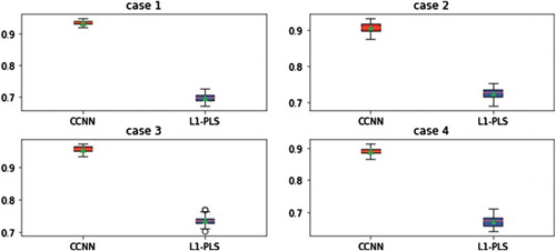
Compared to -pls, CCNN has better performance in terms of overall potential outcome. Value function based on CCNN is larger than that of -pls: in case 1, the value ratio for CCNN and -pls is 1.34. We also notice that the difference between two methods in stage 2 is less than that of stage 1. There are several reasons: the optimal decision rule at stage 1 is more intricate than that of stage 2. Therefore neural network outperforms -pls in approximation of this highly non-linear function. Optimal decision rule at stage 2 can be written as While optimal decision rule at stage 1 is more complicated. Another possible explanation may be optimal decision rule at stage 1 involves fewer covariates, resulting in less noise and more signal. Nevertheless, when the true decision function can be approximated well enough by linear regression, it is possible that -pls may achieve better results.

5. Application to STAR*D study

In this section, we demonstrate the performance of the proposed deep A-learning methods using the STAR*D clinical trial dataset. We compared mean population outcome following the estimated DTR using the deep A-learning and PLS estimator based on a linear decision rule.

5.1. Dataset

STAR*D is the largest and longest clinical trial to compare the effectiveness of treatments for major depressive disorder. It has four levels. Each level lasts for 12 weeks. The severity of depression is measured by Quick Inventory of Depressive Symptomatology (QIDS) score. Participants without adequate clinical response at the end of each level would continue to the next stage. For level 1, all participants received citalopram. For each level of 2–4, patients received one randomised treatment. Covariates are collected from enrolment, IVR call, ROA interviews, clinic visit and other events (such as suicide, non-serious adverse event and protocol deviation). See Fava et al. (2003) for design and measurement details of STAR*D study.

5.2. Processing

In general, there are two types of options: switch to a different medication or adding on to their existing medication. Since all patients received the same treatment at level 1 and the number of patients who entered level 4 is too small, we only focus on the 299 patients that has complete information at level 2 and level 3. Table 1 is the list of treatment switch and treatment augmentation options at the two levels. We take the negative level 3 16-item QIDS (QIDS-C16) as response variable Y. The propensity score is assumed to be constant and is estimated using sample mean. At each level, we remove a few covariates with small variance and reshape the covariate vector to a square matrix. The inputs of CNN/CCNN for level 2 are a matrix and a matrix for level 3 respectively. Local normalisation and zero-phase component analysis (ZCA-whitening) are incorporated for the input data. ZCA-whitening proposed by Krizhevsky and Hinton (2009) is a popular technique for pre-processing of CNN. It can preserve local properties. ZCA-whitening can produce sphered and less-correlated covariates while transforming the data as little as possible. ZCA is summarised in (6(6) ) where Σ is the covariance matrix, whose eigenvalues are and close to the original variable linearly independent eigenvectors are column vectors of matrix P. The regularisation parameter ε is added to avoid numerically unstable situations. (6)

Table 1. Lists of STAR*D treatment options at level 2 and level 3.

Type	Level	Treatment
Switch	2	Bupropion SR, Sertraline, Venlafaxine XR
Augmentation	2	Citalopram plus Bupropion SR, Citalopram plus Buspirone
Switch	3	Nortriptyline, Mirtazapine
Augmentation	3	Lithium augmentation, Triiodothyronine augmentation

5.3. Architecture

The architecture of two-layer CNN is as follows: the filter size of convolutional layer is for stage 2 and for stage 3 since number of covariates at level 3 is larger. The average pooling is implemented in the pooling layer with pooling patch size and pooling stride 2. We do not use any padding techniques in order to control overfitting. Then a fully connected layer maps all neurons to a scalar. For m-layer CNN, it has m−1 convolutional layers followed by one fully connected layer. The number of filters is tuned by IPW estimator of value function: The architecture of CCNN is very similar to CNN except that pooling is taken place before convolution operation. This can reduce the number of parameters in the neural network. The number of dimension of random feature approximation, the scale parameter of Gaussian kernel and the nuclear norm constraint are tuned. Both CNN and CCNN are trained using mini-batch gradient descent. The learning rate of CNN and CCNN are and , respectively. CNN is implemented using tensorflow (Abadi et al., 2015).

5.4. Results

We compare the results based on neural network with -pls. Shrinkage parameter λ is tuned based on BIC. To measure the performance of estimated DTR, we split the data into three parts: 60% of dataset to be training data, 20% as validation and 20% as testing. Since parameters are randomly initialised, the accuracy of DTR varies each time. We trained each architecture 100 times using the training dataset and choose the best network based on the maximum value function estimation on the validation dataset. We report the value function estimation on the testing dataset. Table 2 summarised the results of different architectures.

Table 2. Evaluation results for estimated values on STAR*D dataset.

Methods	Number of layers	Value function estimation
CCNN	2
CCNN	3
CNN	2
CNN	3
CNN	4
-pls	–

Based on the results, we have the following observations. Both CNN and CCNN can learn a DTR that outperforms -pls. They use intricate functions to learn a decision rule. It is more accurate than that of PLS estimator. For fixed number of layers, CCNN has better performance than CNN. We also notice that processing has a great influence on decision accuracy. For example, without zca-whitening, both CNN and CCNN would have smaller estimated value function.

6. Conclusion and future work

In this paper, we propose a deep A-learning framework which integrates CNN and CCNN with A-learning for optimal treatment regime estimation. This method can be applied to situations where medical images are available. Here our contrast function is estimated based on IPW estimator. The new methods have the following advantages. It uses intricate functions to learn decision rules, which allows for model flexibility. The parameter sharing mechanism makes it computational efficient and controls overfitting. Both simulation results and STAR*D application indicate that deep A-learning outperforms PLS estimator. Although deep neural network has shown its competency in intricate scenarios, linear approximation based Q-learning or A-learning may still lead to a more accurate and computational-efficient solution when the true optimal decision rule is simple.

Complicated architectures which consist of multiple subnetworks have demonstrated themselves to be very powerful. An extension for the near future is to study the performance of deep A-learning using these architectures. Adaptive methods for hyperparameter specification are also worth studying. Last but not least, the performance of neural network would improve if training sample size increases. In computer vision, techniques such as rotation and flipping are widely used for data augmentation. Another line of future work is to investigate whether incorporating those techniques can help further improve the performance of optimal DTR estimation.

Disclosure statement

No potential conflict of interest was reported by the authors.

Shuhan Liang is a Ph.D. student in the Department of Statistics at North Carolina State University. Her research interests focus on machine learning and optimal treatment regime estimation.

Wenbin Lu is a professor in the Department of Statistics at North Carolina State University. He received his Ph.D. in Statistics from Columbia University in 2003. His research interests focus on biostatistics, high-dimensional data analysis, and machine and reinforcement learning.

Rui Song is an associate professor in the Department of Statistics at North Carolina State University. She received her Ph.D. in Statistics from the University of Wisconsin at Madison in 2006. Her research interests focus on high-dimensional statistical learning, semiparametric inference and dynamic treatment regime.

Additional information

Funding

This work was supported by National Institutes of Health [5P01CA142538].

Notes

1 The codes used in our paper are adapted from the source codes of Zhang et al. (2016) for CCNN.

References

- Abadi, M., Agarwal, A., Barham, P., Brevdo, E., Chen, Z., Citro, C., … Zheng, X. (2015). TensorFlow: Large-scale machine learning on heterogeneous systems. Retrieved from https://protect-us.mimecast.com/s/fd_CCzpBnGHM4pWNviXNGA_?domain=tensorflow.org. Software available from tensorflow.org.
- Basu, D. (1980). Randomization analysis of experimental data: The fisher randomization test. Journal of the American Statistical Association, 75(371), 575–582. doi: 10.1080/01621459.1980.10477512
- Bojarski, M., Del Testa, D., Dworakowski, D., Firner, B., Flepp, B., Goyal, P., … Zieba, K. (2016). End to end learning for self-driving cars. arXiv preprint arXiv:1604.07316.
- Choromanska, A., Henaff, M., Mathieu, M., Arous, G. B., & LeCun, Y. (2015). The loss surfaces of multilayer networks. AISTATS, 38, 192–204.
- Collobert, R., & Weston, J. (2008). A unified architecture for natural language processing: Deep neural networks with multitask learning. In Proceedings of the 25th international conference on machine learning, Helsinki, Finland (pp. 160–167). ACM.
- Cowell, R. G., Dawid, P., Lauritzen, S. L., & Spiegelhalter, D. J. (2006). Probabilistic networks and expert systems: Exact computational methods for Bayesian networks. New York, NY: Springer Science & Business Media.
- Ding, X., Zhang, Y., Liu, T., & Duan, J. (2015). Deep learning for event-driven stock prediction. In IJCAI, Buenos Aires, Argentina (pp. 2327–2333).
- Duchi, J., Shalev-Shwartz, S., Singer, Y., & Chandra, T. (2008). Efficient projections onto the l 1-ball for learning in high dimensions. In Proceedings of the 25th international conference on machine learning, Helsinki, Finland (pp. 272–279). ACM.
- Fan, J., & Li, R. (2001). Variable selection via nonconcave penalized likelihood and its oracle properties. Journal of the American Statistical Association, 96(456), 1348–1360. doi: 10.1198/016214501753382273
- Fava, M., Rush, J., Trivedi, M. H., Nierenberg, A., Thase, M., Sackeim, F., … Kupfer, D. J. (2003). Background and rationale for the sequenced treatment alternatives to relieve depression (STAR*D) study. Psychiatric Clinics of North America, 26(2), 457–494. doi: 10.1016/S0193-953X(02)00107-7
- Hornik, K., Stinchcombe, M., & White, H. (1989). Multilayer feedforward networks are universal approximators. Neural Networks, 2(5), 359–366. doi: 10.1016/0893-6080(89)90020-8
- Karpathy, A. (2017). Lecture notes in cs231n: Convolutional neural networks for visual recognition. Spring.
- Krizhevsky, A., & Hinton, G. (2009). Learning multiple layers of features from tiny images (MSc thesis).
- Krizhevsky, A., Sutskever, I., & Hinton, G. E. (2012). Imagenet classification with deep convolutional neural networks. In Advances in neural information processing systems (pp. 1090–1098). Cambridge: The MIT Press.
- LeCun, Y., Bengio, Y., & Hinton, G. (2015). Deep learning. Nature, 521(7553), 436–444. doi: 10.1038/nature14539
- LeCun, Y., Bottou, L., Bengio, Y., & Haffner, P. (1998). Gradient-based learning applied to document recognition. Proceedings of the IEEE, 86(11), 2278–2324. doi: 10.1109/5.726791
- Lenz, I., Lee, H., & Saxena, A. (2015). Deep learning for detecting robotic grasps. The International Journal of Robotics Research, 34(4–5), 705–724. doi: 10.1177/0278364914549607
- Lu, W., Zhang, H., & Zeng, D. (2013). Variable selection for optimal treatment decision. Statistical Methods in Medical Research, 22(5), 493–504. doi: 10.1177/0962280211428383
- Mnih, V., Kavukcuoglu, K., Silver, D., Graves, A., Antonoglou, I., Wierstra, D., & Riedmiller, M. (2013). Playing atari with deep reinforcement learning. arXiv preprint arXiv:1312.5602.
- Mnih, V., Kavukcuoglu, K., Silver, D., Rusu, A. A., Veness, J., Bellemare, M. G., … Hassabis, D. (2015). Human-level control through deep reinforcement learning. Nature, 518(7540), 529–533. doi: 10.1038/nature14236
- Moodie, E. E., Richardson, T. S., & Stephens, D. A. (2007). Demystifying optimal dynamic treatment regimes. Biometrics, 63(2), 447–455. doi: 10.1111/j.1541-0420.2006.00686.x
- Murphy, S. A. (2003). Optimal dynamic treatment regimes. Journal of the Royal Statistical Society: Series B, 65(2), 331–355. doi: 10.1111/1467-9868.00389
- Pedregosa, F., Varoquaux, G., Gramfort, A., Michel, V., Thirion, B., Grisel, O., … Duchesnay, E. (2011). Scikit-learn: Machine learning in Python. Journal of Machine Learning Research, 12, 2825–2830.
- Pinkus, A. (1999). Approximation theory of the MLP model in neural networks. Acta Numerica, 8, 143–195. doi: 10.1017/S0962492900002919
- Qian, M., & Murphy, S. A. (2011). Performance guarantees for individualized treatment rules. Annals of Statistics, 39(2), 1180–1210. doi: 10.1214/10-AOS864
- Rahimi, A., & Recht, B. (2007). Random features for large-scale kernel machines. In Advances in neural information processing systems 20 (pp. 1–8). Vancouver: Curran Associates.
- Robins, J. (1997). Causal inference from complex longitudinal data. In Latent variable modeling and applications to causality. New York, NY: Springer.
- Schulte, P. J., Tsiatis, A. A., Laber, E. B., & Davidian, M. (2014). Q-and a-learning methods for estimating optimal dynamic treatment regimes. Statistical Science, 29(4), 640–661. doi: 10.1214/13-STS450
- Shi, C., Fan, A., Song, R., & Lu, W. (2017). High-dimensional a-learning for optimal dynamic treatment regimes. Annals of Statistics, 4(1), 59–68.
- Shi, C., Song, R., & Lu, W. (2016). Robust learning for optimal treatment decision with np-dimensionality. Electronic Journal of Statistics, 10(2), 2894–2921. doi: 10.1214/16-EJS1178
- Silver, D., Huang, A., Maddison, C. J., Guez, A., Sifre, L., Van Den Driessche, G., … Hassabis, D. (2016). Mastering the game of go with deep neural networks and tree search. Nature, 529(7587), 484–489. doi: 10.1038/nature16961
- Song, R., Kosorok, M., Zeng, D., Zhao, Y., Laber, E., & Yuan, M. (2015). On sparse representation for optimal individualized treatment selection with penalized outcome weighted learning. Stat, 4(1), 59–68. doi: 10.1002/sta4.78
- Tibshirani, R. (1996). Regression shrinkage and selection via the lasso. Journal of the Royal Statistical Society. Series B, 58(1), 267–288.
- Watkins, C. J. C. H. (1989). Learning from delayed rewards (PhD thesis). University of Cambridge, England.
- Watkins, C. J., & Dayan, P. (1992). Q-learning. Machine Learning, 8(3–4), 279–292. doi: 10.1007/BF00992698
- Zhang, Y., Liang, P., & Wainwright, M. J. (2016). Convexified convolutional neural networks. arXiv preprint arXiv:1609.01000.
- Zhang, B., Tsiatis, A. A., Davidian, M., Zhang, M., & Laber, E. (2012). Estimating optimal treatment regimes from a classification perspective. Stat, 1(1), 103–114. doi: 10.1002/sta.411
- Zhao, Y., Zeng, D., Rush, J., & Kosorok, M. (2012). Estimating individualized treatment rules using outcome weighted learning. Journal of the American Statistical Association, 107(499), 1106–1118. doi: 10.1080/01621459.2012.695674