
ABSTRACT
In this paper, a generalisation of the exponential distribution, namely, Weibull exponentiated-exponential (WEE) distribution, is proposed. The shapes of the density function possess great flexibility. It can accommodate various hazard shapes such as reversed-J, increasing, decreasing, constant and upside-down bathtub. Various properties of the WEE distribution are studied including shape properties, quantile function, expressions for the moments and incomplete moments, probability weighted moments and Shannon entropy. We obtain the asymptotic distributions for the sample minimum and maximum. The model parameters are estimated by maximum likelihood. The usefulness of the new model is illustrated by means of two real lifetime data sets.
1. Introduction
Gupta, Gupta, and Gupta (Citation1998) introduced the exponentiated-G (‘exp-G’ for short) class of distributions based on Lehmann's ( Citation1953) type I and II alternatives. Gupta and Kundu (Citation1999) studied the two-parameter exponentiated-exponential (EE) distribution as an extension of the exponential distribution based on Lehmann type I alternative. The EE distribution is also known as the generalised exponential (GE) distribution in the literature. Since it is the most attractive generalisation of the exponential distribution, the EE model has received increased attention and many authors have studied its various properties and also proposed comparisons with other distributions. Some significant references are Gupta and Kundu (Citation2001a, Citation2001b, Citation2002, Citation2003, Citation2004, Citation2006, Citation2007, Citation2008, Citation2011), Kundu, Gupta, and Manglick (Citation2005), Nadarajah and Kotz (Citation2006a), Dey and Kundu (Citation2009), Pakyari (Citation2010) and Nadarajah (Citation2011). In fact, the two-parameter EE model has been proven to be a good alternative to other two-parameter distributions such as the gamma, Weibull and log-normal. The EE distribution can be used quite effectively for analysing lifetime data which has monotonic (increasing or decreasing) hazard rate function (hrf) but unfortunately it cannot be used for upside-down bathtub shaped data. Interestingly, the proposed three-parameter distribution has constant, increasing, decreasing and upside-down bathtub shapes and, therefore, it can be used effectively for analysing lifetime data of various shapes. Also, few distributions in the literature can be used to model left-skewed data. However, the proposed distribution can be left-skewed, right-skewed and about symmetric. Section 7 provides illustrations of how the proposed model can be used to fit various shapes including left-skewed data.
Generalising distributions is always precious for applied statisticians and recent literature has suggested several ways of extending well-known distributions. Recently, Alzaatreh, Lee, and Famoye (Citation2013) defined the T-X family of distributions as follows: Let be the pdf of a continuous random variable
for
and let
be a link function which satisfies the two conditions:
(1) The cdf of the T-X family of distributions is given by
(2) where
satisfies the conditions described in Equation (Equation1
(1) ) and
is a cdf of any random variable X. The pdf corresponding to Equation (Equation2
(2) ) is given by
(3)
Now, let T be a continuous random variable defined on
and
. Then the link function,
, satisfies the two conditions in Equation (Equation1
(1) ). Therefore, the cdf of the T-X family reduces to
(4) The pdf corresponding to Equation (Equation4
(4) ) is given by
(5) Note that the pdf in Equation (Equation5
(5) ) can be written as
where
and
are the hazard and cumulative hazard functions associated with
. The family (Equation5
(5) ) allows us to extend well-known distributions and at the same time develop more realistic statistical models with a great flexibility in terms of applications.
The paper is unfolded as follows. In Section 2, we define the Weibull exponentiated-exponential (WEE) distribution. In Section 3, we study some properties of the WEE distribution. In Section 4, we derive explicit expressions for the ordinary and incomplete moments and mgf. The density of the order statistics as well as the asymptotic distributions of the minimum and maximum order statistics is studied in Section 5. In Section 6, the model parameters are estimated by maximum likelihood. Applications to real life data are presented in Section 7. Finally, Section 8 offers some concluding remarks.
2. Model definition
If T follows the Weibull random variable with shape parameter c>0 and scale parameter of 1, say Weibull(c), then its cdf and pdf are given by and
, respectively. From Equation (Equation2
(2) ), the cdf of the Weibull-X family is defined by
(6) The pdf corresponding to Equation (Equation6
(6) ) is given by
(7) Note again that the pdf in Equation (Equation7
(7) ) can be written as
The Weibull-X family has a closed-form cdf. Also, it produces larger skewness ranges (left and right) and its hrf has flexible shapes.
A random variable Z has the exponentiated-exponential (‘EE’ for short) distribution with two parameters α and λ, if its cumulative distribution function (cdf) is given by
(8) The probability density function (pdf) corresponding to Equation (Equation8
(8) ) reduces to
(9) where
and
are the shape and scale parameters, respectively.
Inserting Equation (Equation8(8) ) into Equation (Equation6
(6) ) gives the WEE cdf as
(10) The pdf
corresponding to Equation (Equation10
(10) ) is given by
(11) Henceforth, a random variable having pdf (Equation11
(11) ) is denoted by
.
The hrf of the WEE model is given by
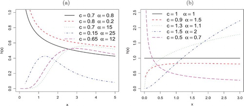
Figures and display some plots of the pdf and hrf of X for some parameter values. Figure reveals that the WEE pdf has various shapes such as symmetric, right-skewed, left-skewed and reversed-J. Also, Figure shows that the WEE hrf can produce failure rate shapes such as constant, increasing, decreasing, upside-down bathtub and reversed-J.
Figure 1. Density function plots of the WEE distribution.
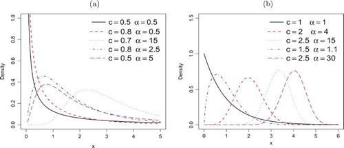
Figure 2. Hazard rate plots of the WEE distribution.
3. Some properties of the WEE distribution
In this section, we provide several properties of the WEE distribution. We omit the proof for some immediate results.
The limiting behaviour of the pdf and hrf of X are given in the following lemma.
Lemma 3.1
The limit of the pdf of X as is 0. Also, the limits of the pdf and hrf of X as
are given by
Further, the limit of the hrf of X as
is given by
Comment 1
The quantile function of the WEE distribution is
(12)
where
One can show immediately from Equation (14) that the mode of
Theorem 3.1
The WEE pdf is an infinite mixture of EE pdfs, namely:
(14) where
is defined below and
is the EE density function with parameters
and λ.
Proof.
Let ,
and
. Then, we can write
(15)
(16)
(17) Here, the constants
(for
and
) can be determined recursively by
where
and
(http://functions.wolfram.com/ElementaryFunctions/Log/06/01/04/03/).
Expression (Equation14(14) ) follows by substituting Equations (Equation15
(15) ) –(Equation17
(17) ) in Equation (Equation11
(11) ).
This expression is very useful to obtain several WEE properties using the properties of the EE model.
Comment 2
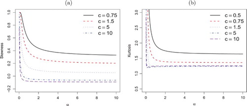
The analysis of the variability of the skewness and kurtosis on the shape parameters α and c can be investigated based on quantile measures. The shortcomings of the classical kurtosis measure are well known. The Bowley skewness (Kenney & Keeping, Citation1962) based on quartiles is given by
The Moors (Citation1998) kurtosis based on octiles is given by
These measures are less sensitive to outliers and they exist even for distributions without moments. In Figure , we plot the measures B and M of the WEE distribution. From the figure for fixed λ, the skewness is a decreasing function of c. The distribution can be left skewed, right skewed and nearly symmetric (B=0).
Figure 3. Skewness (a) and kurtosis (b) of X based on quantiles when .
The Shannon entropy is a measure of variation of uncertainty in a random variable and has wide applications in science, engineering and probability theory. The Shannon (Citation1948) entropy is defined as . The following theorem provides expression for Shannon's entropy for the WEE.
Theorem 3.2
If , then Shannon's entropy of X is given by
(18) where
.
To prove Theorem 3.2, we need the following result from Alzaatreh et al. (Citation2013).
Lemma 3.2
Shannon's entropy for the Weibull-X family in Equation (Equation7(7) ) can be expressed as
(19) where
and
are the cdf and pdf of the Transformer family, respectively, and T follows the Weibull model with shape parameter c and unity scale parameter and ξ is Euler's constant.
Proof.
From Equations (Equation9(9) ) and (Equation8
(8) ), we get
(20) where
Weibull
. Next, we consider
.
Using the power series for , we obtain
(21) Further,
(22) Equation (Equation18
(18) ) follows from Equations (Equation21
(21) ) and (Equation22
(22) ) by substituting Equation (Equation20
(20) ) into Equation (Equation19
(19) ).
The Shannon entropy in Equation (Equation18(18) ) can be used to discriminate between WEE distribution and any other member of Weibull-X family where X does not follow the EE distribution. To see this, let
and
be two random variables with CDFs, respectively, are
and
. One can use Shannon entropy to discriminate between Weibull-
and Weibull-
. The most appropriate model for a given data is the model with the largest Shannon entropy. Consider
, using Equation (Equation19
(19) ) we have
(23) where T follows the Weibull distribution with shape parameter c and scale of 1. The sample
is defined as
Where
, can be obtained from a given data set
Therefore, to test the hypotheses
vs
, reject
at level a if
, where
is the upper
point of the distribution of
under
. Of course, if the purpose is to discriminate between WEE and any other member of Weibull-X family,
and
will be the PDF and quantile function for the WEE and
and
are the PDF and quantile function of the Weibull-X distribution.
4. Moments
In this section, we derive the ordinary, incomplete moments and mgf of the WEE distribution. This task can be easily done using the fact that WEE is an infinite linear combination of EE distributions. Therefore, in order to obtain the moments of WEE, we first obtain the moments of EE distribution. Let Z follows EE distribution in Equation (Equation9
(9) ), then the rth moment of Z is given by
(24) where
The mean and variance of Z are
and
, respectively.
The moment generating function (mgf) of the EE distribution (for ) is given by
(25) where
is the beta function and
(for p>0) is the gamma function.
The rth incomplete moment of Y is given by
(26) where
and
(for p>0) is the incomplete gamma function.
Theorem 4.1
If , then
(i) the rth moment of X can be expressed as
(27) where
and
is defined in Theorem 3.1.
(ii) The mgf of X is
Proof.
For (i), Theorem 3.1 implies that
The result in (i) follows by using Equation (Equation24
(24) ). The proof of (ii) is similar to (i) from Equation (Equation25
(25) ). Hence the proof.
Remark
On setting r=1 in Equation (Equation27(27) ), we obtain the mean
. The central moments (
) and cumulants (
) of X are obtained from Equation (Equation27
(27) ) as
respectively, where
. Thus,
,
,
, etc. The skewness and kurtosis can be calculated from the third and fourth standardised cumulants as
and
. They are also important to derive Edgeworth expansions for the cdf and pdf of the standardised sum and mean of independent and identically distributed random variables having the WEE distribution.
Theorem 4.2
If , then the rth incomplete moment of X is given by
(28) where (for
)
Proof.
Similar to the proof of Theorem 4.1.
Remark
(i) The main application of the first incomplete moment refers to the Bonferroni and Lorenz curves. These curves are very useful in several fields. For a given probability π, they are defined by and
, respectively, where
comes from Equation (Equation28
(28) ) with r=1 and
is determined from Equation (Equation12
(12) ).
(ii) The amount of scatter in a population is measured to some extent by the totality of deviations from the mean and median defined by and
, respectively, where
is the mean and
is the median. These measures can be expressed as
and
, where
comes from Equation (Equation10
(10) ).
(iii) Other applications of the first incomplete moment are related to the mean residual life and mean waiting time given by and
, respectively, where
and
are obtained from Equation (Equation10
(10) ).
The th probability weighted moment (PWM) of X (for
) is formally defined by
(29) Some important features of PWM are that unlike conventional moments they do not require higher moments for consistency, their finite mean can be used for estimation consistency, they are less sensitive to outliers, uniquely determine a distribution and relatively good at capturing the middle of a distribution. For some specific distributions, the relations between the PWMs and the parameters are of a simpler analytical structure than those between the conventional moments and the parameters. The simpler analytical structure suggests that it may be possible to derive relations between the parameters and the PWMs even though it may not be possible to obtain relations between the parameters and the conventional moments.
Theorem 4.3
If , then the PWMs of X are given by
where
and
is defined in Theorem 4.2.
Proof.
Consider
Using the generalised binomial expansion, we obtain
(30) Inserting Equations (Equation11
(11) ) and (Equation30
(30) ) into Equation (Equation29
(29) ) and, after some expansion,
can be expressed as
The proof ends by using Equation (Equation27
(27) ).
5. Order statistics
In this section, we provide the density of the ith-order statistic ,
say, in a random sample of size n from the WEE distribution. By suppressing the parameters, we have (for
)
(31) On using Equations (Equation10
(10) ) and (Equation11
(11) ) in Equation (Equation31
(31) ), we obtain
(32) where
and
denotes the WEE density function with parameters
, α and λ. So, the density function of the WEE order statistics is a mixture of WEE densities. Based on Equation (Equation32
(32) ), we can obtain some structural properties of
from those WEE properties.
Let us consider the asymptotic distributions of the sample maximum and sample minimum
. In order to derive the asymptotic distribution of the sample minimum
, we consider Theorem 8.3.6 of Arnold, Balakrishnan, and Nagarajah (Citation2008). Note that, since
, the asymptotic distribution of
is the Weibull distribution with shape parameter
and unit scale parameter if
By using Equation (Equation11
(11) ), we have
Hence, we conclude that the asymptotic distribution of the sample minimum
is of the Weibull type with shape parameter
and unit scale parameter.
In order to obtain the large sample distribution of , we use the sufficient condition for weak convergence due to (von Mises, Citation1936), which is stated in the following theorem:
Theorem 5.1
Let G be an absolutely continuous cdf and suppose is a nonzero and differentiable function. If
then
, where
.
Proof.
In our case, and it is easy to prove that
Hence, the large sample distribution of
is of the extreme value type.
6. Estimation and simulation study
In this section, we consider the estimation of the unknown parameters of the WEE distribution by using the maximum likelihood method. Let be a sample of size n from the WEE distribution in Equation (Equation11
(11) ). The log-likelihood function for the vector of parameters
can be expressed as
where
The log-likelihood function can be maximised numerically to obtain the MLEs. The initial values for the parameters λ and α can be taken by fitting the data to the EE distribution in Equation (2). The initial value for the parameter c can be taken as 1. There are various routines available for numerical maximisation. The elements of the observed information matrix are given in Appendix. In this paper, we use the OPTIM routine in the R software. For interval estimation of the parameters, we require the observed information matrix
(for
). Under standard regularity conditions, the multivariate normal
distribution can be used to construct approximate confidence intervals for the model parameters. Here,
is the total observed information matrix evaluated at
. Then, the
confidence intervals for c, α and λ are given by
,
, and
, respectively, where the
's denote the diagonal elements of
corresponding to the model parameters, and
is the quantile (
) of the standard normal distribution.
The likelihood ratio (LR) statistic can be used to check if the WEE distribution is strictly ‘superior’ to the EE distribution for a given data set. Then, the test of vs
is not true is equivalent to compare the WEE and EE distributions and the LR statistic becomes
, where
,
and
are the MLEs under
and
and
are the estimates under
.
6.1. Simulation study
In this section, we evaluate the performance of the MLEs by using Monte Carlo simulation for different sample sizes and different parameter values. The simulation study is repeated N=5000 times each with sample sizes and parameter combinations I: c=0.5,
,
, II: c=0.5,
,
and III: c=1.5,
,
. The estimated bias(Bias), mean square error (MSE) and coverage probability (CP) can be obtained using the following equations:
Table presents the average bias(Bias), MSE, CP, average lower bound (LB) and average upper bound (UB) values of the parameters c, α and λ for different sample sizes. From the results, we can verify that the Bias and MSEs decreases as the sample size n increases. The CP of the confidence intervals are quite close to the nominal level of 95%. Therefore, the MLEs and their asymptotic results can be used for estimating and constructing confidence intervals even for reasonably small sample sizes.
Table 1. Monte Carlo simulation results: Bias, MSE, CP, LB and UB.
7. Applications
In this section, we fit the WEE model to two real data sets with different highly skewness values (right and left skewness). We compare its fits with two and three-parameter distributions, namely, the gamma-exponentiated exponential (GEE) (Ristić & Balakrishnan, Citation2012) and beta-exponential (BE) (Nadarajah & Kotz, Citation2006b). The density functions for the GEE and BE are, respectively, given by
The method of maximum likelihood is used to estimate the unknown parameters for the models. Tables and list the MLEs and their corresponding standard errors (in parentheses) for the model parameters.
Table 2. MLEs and their standard errors (in parentheses) for the guinea pigs data.
Table 3. MLEs and their standard errors (in parentheses) for the glass fibres data.
Data set 1: guinea pigs data
The first data set corresponds to the survival times (in days) of 72 guinea pigs infected with virulent tubercle bacilli reported by Bjerkedal (Citation1960). The data are: 12, 15, 22, 24, 24, 32, 32, 33, 34, 38, 38, 43, 44, 48, 52, 53, 54, 54, 55, 56, 57, 58, 58, 59, 60, 60, 60, 60, 61, 62, 63, 65, 65, 67, 68, 70, 70, 72, 73, 75, 76, 76, 81, 83, 84, 85, 87, 91, 95, 96, 98, 99, 109, 110, 121, 127, 129, 131, 143, 146, 146, 175, 175, 211, 233, 258, 258, 263, 297, 341, 341, 376. A summary of these data is:
s=81.1180,
Data set 2: glass fibres data
The third data set represents the strength of 1.5 cm glass fibres measured at National Physical laboratory, England (Smith & Naylor, Citation1987). The data are: 0.55, 0.93, 1.25, 1.36, 1.49, 1.52, 1.58, 1.61, 1.64, 1.68, 1.73, 1.81, 2.00, 0.74, 1.04, 1.27, 1.39, 1.49, 1.53, 1.59, 1.61, 1.66, 1.68, 1.76, 1.82, 2.01, 0.77, 1.11, 1.28, 1.42, 1.50, 1.54, 1.60, 1.62, 1.66, 1.69, 1.76, 1.84, 2.24, 0.81, 1.13, 1.29, 1.48, 1.50, 1.55, 1.61, 1.62, 1.66, 1.70, 1.77, 1.84, 0.84, 1.24, 1.30, 1.48, 1.51, 1.55, 1.61, 1.63, 1.67, 1.70, 1.78, 1.89. A summary of these data is:
s=0.3241,
In order to compare the models, we adopt the following statistics: Akaike information criterion (AIC), Bayesian information criterion (BIC), Anderson– Darling (), Cramér–von Mises (
) and
Kolmogorov–Smirnov (K–S) statistic (with p-values ). In general, the smaller the values of these statistics, the better the fit to the data. These results are presented in Tables and .
Table 4. The statistics AIC, BIC, , , K–S and K–S p-value for the guinea pigs data.
Table 5. The statistics AIC, BIC, , , K–S and K–S p-value for the glass fibres data.
From the figures in Tables and , we conclude that the WEE model provides the best fit with lowest values of the AIC, BIC, ,
and K–S statistics and largest p-value for the guinea pigs data. For the glass fibres data, GEE and BE do not provide an adequate fit. The summary statistics for both data sets reveal that the guinea pigs data is highly positively skewed data and the
glass fibres data is highly negatively skewed data. This indicates that the WEE distribution can be used to model data with right-skewness and left-skewness characteristic. The QQ plots for both data sets are displayed in Figures and . The plots support the results in Tables and . Furthermore, to identify the hazard shapes of data, we consider the graphical method based on total time on test (TTT) transformed pioneered by Barlow and Campo (Citation1975). The empirical illustration of the TTT transform is given by Aarset (Citation1987). This graph is obtained by plotting
versus
, where
(for
) are the order statistics of the sample. From Figure (a), the
TTT plot for the first data set shows that the hazard function is first concave and then convex giving an indication of upside-down bathtub shape, while the TTT plot in Figures (b) shows that the hazard function is concave giving an indication of increased hazard rate. Hence, the WEE distribution could be in principle an appropriate model for fitting these data sets.
Figure 4. QQ-plot of data set 1.
Figure 5. QQ-plot of data set 2.
Figure 6. TTT plots (a) and (b) data sets 1 and 2.
8. Concluding remarks
In this paper, a new generalisation of the exponential distribution is proposed. The density and hazard functions show a great flexibility. Some of the general properties for the proposed distribution are studied such as mixture representation for the density function, ordinary and incomplete moments, quantile function, probability weighed moments and order statistics. The maximum likelihood method is employed for estimating the model parameters. The proposed model is fitted to highly skewed data sets and the results indicate that the new model is a suitable model to fit data with right-skewed and left-skewed characteristics.
Acknowledgements
The authors would like to thank the Editor-in-Chief and the referee for constructive comments that helped in improving the earlier version of the article.
Disclosure statement
No potential conflict of interest was reported by the authors.
ORCID
M. H. Tahir http://orcid.org/0000-0002-2157-3997
Manat Mustafa http://orcid.org/0000-0002-2967-9008
Additional information
Notes on contributors
Muhammad Zubair
Muhammad Zubair is currently Lecturer in Statistics at Government S.E. College Bahawalpur, Pakistan. He received MSc and MPhil degrees in Statistics from the Islamia University of Bahawalpur (IUB) in 2004 and 2013. Mr. Zubair is PhD candidate in the subject of Statistics at IUB and working under the supervision of Dr. M.H. Tahir. He has 20 publications to his credit.
Ayman Alzaatreh
Dr. Ayman Alzaatreh is currently an Associate Professor at the American University of Sharjah, UAE. Previously, he held an Associate Professor position at the Department of Mathematics at Nazarbayev University. He also served as an Instructor of Mathematics at the University of Jordan and Assistant Professor in the Department of Mathematics and Statistics at Austin Peay State University in Tennessee, USA. His current research focuses on generalising statistical distributions arising from the hazard function. Other research areas include statistical inference of probability models, characterisation of distributions, bivariate and multivariate weighted distributions and Data Mining.
M. H. Tahir
M. H. Tahir is currently Professor of Statistics and Chair, Department of Statistics at the Islamia University of Bahawalpur (IUB), Pakistan. He received MSc and PhD in Statistics in 1990 and 2010, respectively, from IUB. He has been teaching in the Department of Statistics (IUB) since 1992. His current research interests include generalised classes of distributions and their special models, compounded and cure rate models. Dr. Tahir has produced 50 MPhil and 03 PhDs. He is currently supervising 07 PhD students and has more than 60 international publications to his credit.
Muhammad Mansoor
Dr. Muhammad Mansoor is currently Assistant Professor of Statistics at Government Degree College Liaquatpur, Pakistan. He received MSc and MPhil degrees in Statistics from the Islamia University of Bahawalpur (IUB) in 2005 and 2013. Mr. Mansoor has earned PhD in Statistics in 2017 from IUB under the supervision of Dr. M.H. Tahir and has 23 publications to his credit.
Manat Mustafa
Dr. Manat Mustafa received PhD in mathematics from Al-Farabi Kazakh National University in 2012 in Almaty. He is currently an assistant professor at the Department of Mathematics at Nazarbayev University. Prior to joining Nazarbayev University, he served in the School of Physics and Mathematics at Nanyang Technological University in Singapore as a research fellow in 2003--2009, he was a high school math teacher at Republican Specialised Physics-Mathematics Secondary Boarding School for Gifted Students named after O. Zhautykov in Almaty. His research interests include Mathematical logic, computability theory, set theory, and Algebra and operator theory.
References
- Aarset, M. V. (1987). How to identify bathtub hazard rate. IEEE Transactions on Reliability, 36, 106–108. doi: 10.1109/TR.1987.5222310
- Alzaatreh, A., Lee, C., & Famoye, F. (2013). A new method for generating families of continuous distributions. Metron, 71, 63–79. doi: 10.1007/s40300-013-0007-y
- Arnold, B. C., Balakrishnan, N., & Nagarajah, H. N. (2008). A first course in order statistics. New York: Wiley.
- Barlow, R. E., & Campo, R. A. (1975). Total time on test processes and applications to failure data analysis. In: R. E. Barlow, J. B. Fussel, & N. D. Singpurwalla (Eds.), Reliability and fault tree analysis (pp. 451–481). Philadelphia: Society for Industrial and Applied Mathematics.
- Bjerkedal, T. (1960). Acquisition of resistance in guinea pigs infected with different doses of virulent tubercle bacilli. American Journal of Hygiene, 72, 130–148.
- Dey, A. K., & Kundu, D. (2009). Discriminating among the log-normal, Weibull and generalized exponential distributions. IEEE Transactions on Reliability, 58, 416–424. doi: 10.1109/TR.2009.2019494
- Gupta, R. C., Gupta, P. I., & Gupta, R. D. (1998). Modeling failure time data by Lehmann alternatives. Communications in Statistics – Theory and Methods, 27, 887–904. doi: 10.1080/03610929808832134
- Gupta, R. D., & Kundu, D. (1999). Generalized exponential distribution. Australian & New Zealand Journal of Statistics, 41, 173–188. doi: 10.1111/1467-842X.00072
- Gupta, R. D., & Kundu, D. (2001a). Generalized exponential distribution: An alternative to Gamma and Weibull distributions. Biometrical Journal, 43, 117–130. doi: 10.1002/1521-4036(200102)43:1<117::AID-BIMJ117>3.0.CO;2-R
- Gupta, R. D., & Kundu, D. (2001b). Generalized exponential distribution: Different methods of estimations. Journal of Statistical Computation and Simulation, 69, 315–337. doi: 10.1080/00949650108812098
- Gupta, R. D., & Kundu, D. (2002). Discriminating between the Weibull and the GE distributions. Computational Statistics and Data Analysis, 43, 179–196. doi: 10.1016/S0167-9473(02)00206-2
- Gupta, R. D., & Kundu, D. (2003). Closeness of gamma and generalized exponential distributions. Communications in Statistics– Theory and Methods, 32, 705–721. doi: 10.1081/STA-120018824
- Gupta, R. D., & Kundu, D. (2004). Discriminating between the gamma and generalized exponential distributions. Journal of Statistical Computation and Simulation, 74, 107–121. doi: 10.1080/0094965031000114359
- Gupta, R. D., & Kundu, D. (2006). On comparison of the Fisher information of the Weibull and GE distributions. Journal of Statistical Planning and Inference, 136, 3130–3144. doi: 10.1016/j.jspi.2004.11.013
- Gupta, R. D., & Kundu, D. (2007). Generalized exponential distribution: Existing results and some recent developments. Journal of Statistical Planning and Inference, 137, 3537–3547. doi: 10.1016/j.jspi.2007.03.030
- Gupta, R. D., & Kundu, D. (2008). Generalized exponential distribution: Bayesian Inference. Computational Statistics and Data Analysis, 52, 1873–1883. doi: 10.1016/j.csda.2007.06.004
- Gupta, R. D., & Kundu, D. (2011). An extension of generalized exponential distribution. Statistical Methodology, 8, 485–496. doi: 10.1016/j.stamet.2011.06.003
- Kenney, J., & Keeping, E. (1962). Mathematics of statistics (Vol. 1, 3rd ed.). Princeton, NJ: Van Nostrand.
- Kundu, D., Gupta, R. D., & Manglick, A. (2005). Discriminating between the log-normal and the generalized exponential distributions. Journal of Statistical Planning and Inference, 127, 213–227. doi: 10.1016/j.jspi.2003.08.017
- Lehmann, E. L. (1953). The power of rank tests. Annals of Mathematical Statistics, 24, 23–43. doi: 10.1214/aoms/1177729080
- Moors, J. J. A. (1998). A quantile alternative for kurtosis. The Statistician, 37, 25–32. doi: 10.2307/2348376
- Nadarajah, S. (2011). The exponentiated exponential distribution: A survey. AStA Advances in Statistical Analysis, 95, 219–251. doi: 10.1007/s10182-011-0154-5
- Nadarajah, S., & Kotz, S. (2006a). The exponentiated-type distributions. Acta Applicandae Mathematica, 92, 97–111. doi: 10.1007/s10440-006-9055-0
- Nadarajah, S., & Kotz, S. (2006b). The beta exponential distribution. Reliability and Engineering System Safety, 91, 689–697. doi: 10.1016/j.ress.2005.05.008
- Pakyari, R. (2010). Discriminating between generalized exponential, geometric extreme exponential and Weibull distribution. Journal of Statistical Computation and Simulation, 80, 1403–1412. doi: 10.1080/00949650903173306
- Ristić, M. M., & Balakrishnan, N. (2012). The gamma-exponentiated exponential distribution. Journal of Statistical Computation and Simulation, 82, 1191–1206. doi: 10.1080/00949655.2011.574633
- Shannon, C. E. (1948). A mathematical theory of communication. Bell System Technical Journal, 27, 379–432. doi: 10.1002/j.1538-7305.1948.tb01338.x
- Smith, R. L., & Naylor, J. C. (1987). A comparison of maximum likelihood and Bayesian estimators for the three-parameter Weibull distribution. Applied Statistics, 36, 358–369. doi: 10.2307/2347795
- von Mises, R. (1936). La distribution de la plus grande de n valeurs. Revue Mathematique de lUnion Interbalcanique, 1, 141–160.
Appendix
The elements of the observed information matrix
(for
) are given by
where