Objective Bayesian hypothesis testing and estimation for the intraclass model

ABSTRACT

The intraclass correlation coefficient (ICC) plays an important role in various fields of study as a coefficient of reliability. In this paper, we consider objective Bayesian analysis for the ICC in the context of normal linear regression model. We first derive two objective priors for the unknown parameters and show that both result in proper posterior distributions. Within a Bayesian decision-theoretic framework, we then propose an objective Bayesian solution to the problems of hypothesis testing and point estimation of the ICC based on a combined use of the intrinsic discrepancy loss function and objective priors. The proposed solution has an appealing invariance property under one-to-one reparametrisation of the quantity of interest. Simulation studies are conducted to investigate the performance the proposed solution. Finally, a real data application is provided for illustrative purposes.

KEYWORDS:

• Intraclass correlation coefficient
• Bayesian reference criterion
• intrinsic discrepancy
• hypothesis testing
• intrinsic estimator
• reference priors

1. Introduction

Consider the intraclass model of the form (1) where is a vector of response variables, is a design matrix of regressors (assuming the first column is ones) and is a vector of unknown common regression coefficients. We assume that the random error , where stands for ‘independent and identically distributed', is a vector of zeros, and with being a identity matrix and being a matrix containing only ones. The parameter ρ is often referred as the intraclass correlation coefficient (ICC). Note that is the necessary and sufficient condition for positive-definiteness of . When ρ is equal to 0, the intraclass model becomes the classical linear normal model with independent errors.

The ICC has been widely applied in various fields of study as a coefficient of reliability, from epidemiologic research to genetic studies; see, for example Barkto (1966), Fleiss (1986), Lin, Hedayat, Sinha, Yang (2002), among others. The analysis of the ICC transitionally consists of two branches, hypothesis testing and point estimation, and it has received attentions from two main statistical streams of thought: frequentists and Bayesians. From a frequentist viewpoint, Paul (1990) considered the maximum likelihood estimate (MLE) of the ICC in a generalised model setting by solving iteratively a single estimating equation. Paul (1996) developed the score tests for testing the significance of the interclass correlation in familial data. For Bayesian methods, Jelenkowska (1998) studied Bayesian estimation of the ICC in the linear mixed model. Chung and Dey (1998) considered Bayesian analysis of the ICC using the reference prior under a balanced variance components model. Later on, Ghosh and Heo (2003) considered Bayesian credible intervals for ρ based on different objective priors and made comparisons among these priors in terms of matching the corresponding frequentist coverage probabilities.

It deserves mentioning that the problems of hypothesis testing and point estimation for ρ have not yet been studied within a decision-theoretical viewpoint. This motivates us to propose an objective Bayesian solution to these problems based on the Bayesian reference criterion (for short, BRC) (Bernardo & Rueda, 2002). The proposed solution allows the researchers to simultaneously study important inference summaries of the ICC, including point estimation, credible interval estimation and precise hypotheses. In addition, it enjoys various appealing properties: (i) it is invariant under one-to-one reparametrisation of the parameter of interest ρ; (ii) it depends only on the assumed model, appropriate objective priors and the observed data; (iii) it is appropriate to perform the hypothesis test: for any and (iv) it can be easily approximated numerically in most statistical software and can thus be implemented by the practitioners from different fields.

The remainder of the paper is organised as follows. In Section 2, we derive two objective priors of the unknown parameters and discuss the propriety of their corresponding posterior distributions. In Section 3, we propose an objective Bayesian solution to both hypothesis testing and estimation problems of ρ from a decision-theoretical viewpoint. Section 4 investigates the performance of the proposed solution through simulations and a real data application. Some concluding remarks are provided in Section 5, with additional proofs given in the Appendix.

2. Posterior distribution

For notational convenience, let and be vectors and is an design matrix, and they are given by respectively. The model in (1(1) ) can be expressed in a more compact way as (2) where follows an nk-dimensional normal distribution with mean vector and covariance matrix , where is an nk-dimensional matrix and ⊗ denotes the Kronecker product. The likelihood function of the intraclass model in (2(2) ) is given by where denotes the determinant of a matrix .

Bayesian analysis begins with prior specification for all the unknown parameters in the model. In the absence of relevant prior knowledge for in the above model, noninformative priors are often preferred. One of the most popular noninformative priors is the Jeffreys prior, which is proportional to the square root of the determinant of the Fisher information matrix. It can be shown that the Jeffreys prior is given by (3) Given that the parameter of interest is ρ, we integrate out and (i.e., ) and obtain the marginal posterior density for ρ, denoted by , where D represents the observable data. It follows that (4) where . Note that when , the prior in (4(4) ) can be simplified by replacing with , where and . The simplified version is just the Jeffreys prior derived by Ghosh and Heo (2003).

One may argue that, when we aim at a subset of the parameters with the rest treated as nuisance parameters, the direct use of the Jeffreys prior may sometimes be unsatisfactory. To overcome such a pitfall, Bernardo (1979) proposed an algorithm to derive objective priors by maximising some entropy distances. This was further explored by Berger and Bernardo (1992a, 1992b) and named by them the reference priors. We obtain that the one-at-a-time reference prior for the parameter ordering or is given by (5) which is exactly the same as the reference prior identified by Ghosh and Heo (2003), because their model is just a special case of model in (1(1) ) when we set . In addition, it can be shown that the prior in (5(5) ) is a second-order matching prior because it achieves approximate frequentist validity of the posterior quantiles of the interest parameter ρ with a margin of error of . We refer the interested readers to Datta and Ghosh (1995b), Datta and Ghosh (1995a) and Datta and Mukerjee (2004) about the second-order matching criterion in detail. The resulting marginal posterior density of ρ under this prior, denoted by , is given by (6) Given that neither in (3(3) ) nor in (5(5) ) is proper, it is important to study the propriety of their corresponding posterior distributions, which is summarised in the following theorem with proofs given in the Appendix.

Theorem 2.1

Consider the intraclass linear model in (1(1) ). Under either the Jeffreys prior in (3(3) ) or the reference prior in (5(5) ) for the unknown parameters, the joint posterior distribution of is proper when .

As commented by Bernardo (2010), the problems of hypothesis testing and point estimation can be viewed as a special decision problem from a Bayesian decision-theoretic point of view. The choice of the loss function plays a central role in the statistical decision theory. There are numerous loss functions, such as the squared error loss, the zero-one loss and the absolute error loss, whereas many of them often lack the invariance property required in practice. For example, the squared error loss is often overused in statistical inference as a measure of the discrepancy between two sampling distributions, heavily depending on the chosen parameterisations (Bernardo, 2005). In this paper, we consider the intrinsic discrepancy as a loss function due to its various appealing properties discussed in the next section.

3. Bayesian reference criterion

In this section, we propose an objective Bayesian solution based on the BRC proposed by Bernardo and Rueda (2002). In Section 3.1, we overview the BRC and derive the intrinsic discrepancy for the hypothesis testing of ρ. We then obtain Bayesian intrinsic statistic in Section 3.2 and Bayesian intrinsic estimator of ρ in Section 3.3.

3.1. Intrinsic discrepancy loss function

Without loss of generality, we assume that the probabilistic behaviour of observable data can be appropriately described by the probability model (7) where is the parameter of interest and is a nuisance parameter. We aim at deciding whether or not to treat the reduced model under as a proxy for the general model M. In other words, we decide whether the model under is compatible with the observable data. Since the Kullback–Leibler (KL) direct divergence is a good measure of discrepancy between two probability distributions (Robert, 1996), Bernardo (1999) developed the logarithmic discrepancy derived by minimising this divergence measure. Given that the logarithmic discrepancy is not symmetric and this feature may be unsuitable in some contexts, Bernardo and Rueda (2002) developed a symmetric version, often called the intrinsic discrepancy given by where and The unit of the intrinsic discrepancy is the nat of information, while it could be a bit of information if the logarithm was taken in base 2 instead of base e. The intrinsic discrepancy has an invariant property under one-to-one reparametrisation. For a thorough discussion of other properties, see Bernardo and Rueda (2002), Bernardo and Juárez (2003) and Bernardo (2010). In what follows, we provide the intrinsic discrepancy between two intraclass models with its derivations given in the Appendix.

Theorem 3.1

The intrinsic discrepancy for testing versus for under the intraclass model in (1(1) ) is given by (8) where (9)

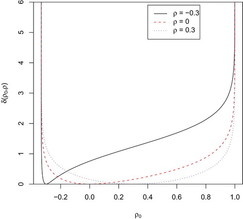
It can be easily verified that is a continuous convex function with a unique minimum at . Figure 1 depicts the curves for n=1, k=4 and . We observe that the corresponding curve of the intrinsic discrepancy always vanishes at .

Figure 1. The intrinsic discrepancy in (8(8) ) as a function of for n=1, k=4 and .

3.2. Bayesian intrinsic statistic

If we select the intrinsic discrepancy as the loss function, then the intrinsic statistic can be defined as the posterior expectation of the intrinsic discrepancy loss, namely, (10) where is the marginal posterior distribution for ρ under the δ-reference prior when the quantity of interest is in (8(8) ). Because is a one-to-one piecewise function of ρ, we follow Proposition 1 of Bernardo (1999) and show that the δ-reference prior corresponding to the parameter of interest is exactly the same as the reference prior for ρ corresponding to the parameter of interest ρ. In addition, the posterior distribution of ρ is invariant under this kind of transformations (Bernardo & Smith, 1994, p. 326). The intrinsic statistic in (10(10) ) can thus be rewritten as where is the marginal posterior distribution of ρ under either in (3(3) ) or in (5(5) ). We observe from Bernardo (2010) that the intrinsic statistic can be interpreted as the expected value of the log-likelihood ratio against the simplified model under . On the other hand, the BRC can be defined as for some given utility constant . In this paper, we advocate the conventional choices for scientific communication. The value of about indicates some evidence against ; the value of about provides rather strong evidence against , while the value of about can be safely used to reject . For further details about these values, we refer the interested readers to Bernardo and Rueda (2002), Bernardo and Juárez (2003), Bernardo and Pérez (2007) and Bernardo (2010).

3.3. Bayesian intrinsic estimator

We follow Bernardo and Juárez (2003) and define the intrinsic estimator of ρ as (11) which is the value minimising the posterior expectation of the intrinsic discrepancy loss function. The intrinsic estimator inherits the invariance property of the intrinsic statistic under one-to-one piecewise transformation, which means that if is a one-to-one reparametrisation of ρ, then the intrinsic estimator of ψ is simply .

4. Examples

We examine the performance of the proposed solution to both hypothesis testing and point estimation problems of ρ through simulation studies ( Section 4.1) and a real data application (Section 4.2).

4.1. Simulation study

We conduct simulation studies to investigate the behaviour of the proposed solution under different scenarios. There are n observations and 2 regressors (p=3) and the data are generated from the model in (1(1) ). Without loss of generality, we set , and , where is the prespecified true value of ICC. Each element of for is generated from a uniform density over the interval , . To check the variations of the proposed approach, is taken to be one of four different values: , 0, 0.3, 0.8 corresponding to the correlation being negative, zero, medium and large, respectively, while considering different sample sizes n=5 (small) and n=20 (medium). For each simulation setting, we consider N=10,000 replications. We analyse the averaged estimates along with the mean absolute errors (MAE) given by where represents the estimate of in jth replication.

The MAEs of the Bayesian estimations and the MLE (Paul, 1990) are reported in Tables 1 and 2. Several features can be drawn as follows. (i) The intrinsic estimator under outperforms the one under in most cases, especially when the sample size is small, and they behave similarly as n increases. (ii) The intrinsic estimator under each prior outperforms the posterior mode and is comparable with the posterior median. (iii) When the true value is near by 0, the MLE performs the best, whereas when is far from 0 (e.g., ), the intrinsic estimator performs the best among all the estimators under consideration. (iv) On average, the MAEs of all the estimators decrease significantly with an increasing sample size. In a marked contrast with other estimators, the intrinsic one is invariant under one-to-one transformation, which is not shared by others, such as the posterior mean. Simulations with other choices of ρ have also been conducted, and similar conclusions are achieved and thus not presented here for simplicity.

Table 1. The MAE of the Bayesian estimators for ρ based on 10,000 replications in the simulation study.

		n=5				n=20
	Prior	Intrinsic	Mean	Median	Mode	Intrinsic	Mean	Median	Mode
		0.148	0.155	0.149	0.162	0.058	0.060	0.058	0.059
		0.164	0.163	0.166	0.185	0.060	0.060	0.060	0.062
0		0.242	0.213	0.243	0.333	0.108	0.105	0.108	0.115
		0.294	0.263	0.296	0.379	0.114	0.111	0.114	0.121
0.3		0.268	0.230	0.268	0.377	0.119	0.115	0.119	0.129
		0.315	0.276	0.315	0.412	0.124	0.119	0.124	0.133
0.8		0.148	0.157	0.148	0.151	0.057	0.059	0.057	0.057
		0.142	0.141	0.141	0.153	0.056	0.056	0.056	0.058

Table 2. The MAE of the MLE for ρ based on 10,000 replications in the simulation study.

	n=5	n=20
	0.137	0.058
0	0.198	0.102
0.3	0.231	0.118
0.8	0.236	0.074

We further compare the frequentist coverage probability of the posterior distributions of ρ under and . Following Sun and Ye (1996), we let α be the left tail probability and be the corresponding quantile of the marginal posterior distribution under either or . Theoretically, it follows . Letting , we observe that should be very close to α if the chosen prior performs well with respect to the probability matching criterion. Table 3 shows the estimated tail probabilities of the posterior distributions between two priors under different scenarios. We observe that the tail probabilities of the posterior distribution of ρ under are closer to the frequentist coverage probabilities than the ones under . This observation is reasonable, because is a second-order matching prior if ρ is the parameter of interest.

Table 3. The estimated tail probabilities of posterior distributions based on 10,000 replications in the simulation study.

		n=5		n=20
	Prior
		0.0453	0.9127	0.0477	0.9010
		0.0497	0.9145	0.0425	0.9166
0		0.0460	0.9069	0.0535	0.8977
		0.0842	0.8598	0.0617	0.8879
0.3		0.0439	0.9119	0.0453	0.9054
		0.1021	0.8357	0.0614	0.8816
0.8		0.0441	0.9087	0.0484	0.9001
		0.1341	0.7825	0.0779	0.8587

In addition to the parameter estimation, the proposed solution can be used to test any value of since k=3 in our simulation study. For illustrative purposes, suppose that we are interested in evaluating whether the data are compatible with . We analyse the frequentist behaviour of the proposed solution under for the hypothesis testing of ρ based on two scenarios discussed below.

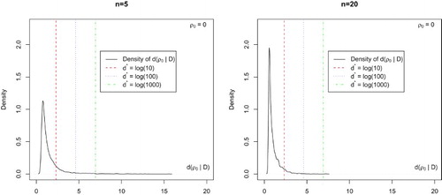
First, consider the scenario in which is true. We simulate 5000 random samples from the model in (1(1) ) with based on the simulation setup above. Figure 2 depicts the sampling distribution of from the 5000 simulations. For n=5, the significance level is around for (mild evidence); the significance level is around for (strong evidence) and the significance level is around for (safe to reject ). We observe that as n increases (n=20), the significance level approximately goes down to , and , respectively. As one would expect, the significance level significantly decreases as n increases from a frequentist viewpoint.

Figure 2. Sampling distribution of under obtained from the 5000 simulations with for different sample sizes when testing .

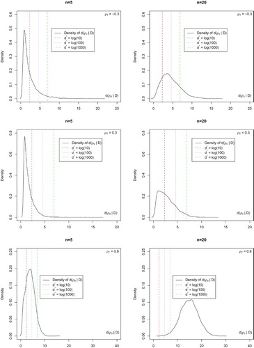
Second, consider the scenario in which is not true. We study the behaviour of the sampling distribution of the proposed solution and the relative frequency of the rejection of . We again simulate 5000 random samples from the model in (1(1) ) with . Figure 3 shows the sampling distribution of from the 5000 simulations. Note that the power of the proposed approach increases when is far from the testing value or n is larger. For instance, when while , for n=5, the relative frequency of rejecting is approximately equal to for , to for , and to for ; for n=20, this relative frequency significantly increases to , and , respectively. We may thus conclude that the power of the proposed solution increases with n and that the performance of the proposed solution is quite satisfactory for the problems of hypothesis testing and point estimation of ρ in the intraclass model in (1(1) ).

Figure 3. Sampling distribution of under obtained from 5000 simulations with for different sample sizes when testing .

Given that there are two objective priors: the reference prior () or the Jeffreys prior (), which of them is preferable for the proposed solution in practical applications? Numerical evidence from the above simulation studies showed that the Bayesian estimations under outperform the ones under . Additionally, is also a second-order matching prior if ρ is the parameter of interest. We thus have a preference to recommend the use of in the analysis of the ICC.

4.2. An illustrative example

We use a real data example to illustrate the practical application of the proposed solution. The orthodontic data set is present in Table 4 and obtained from Chapter 5.2 of Frees (2004): 27 individuals including 16 boys and 11 girls were measured for distances from the pituitary to the pteryomaxillary fissure in millimetres, at ages 8, 10, 12 and 14. We consider the intraclass model of the form where with being the distance for individual i measured at age j, is a vector of ages and represents the gender (1 for male and 0 for female), and with . We observe from Figure 4(a) that the marginal posterior densities for ρ under two objective priors are quite normal in shape. Table 5 provides the point estimators for ρ under different procedures. We here analyse the results under for simplicity. The intrinsic estimator is close to the posterior median equal to 0.620, whereas both are slightly different from the MLE equal to 0.597. According to the non-rejection regions with presented in Figure 4(b), we somehow doubt that the true value of ρ is outside ; we seriously doubt that ρ is outside , and we are almost sure that the true correlation value ρ is not outside .

Figure 4. The marginal posterior density for ρ based on two objective priors (left), and the intrinsic statistic with the non-rejection regions corresponding to the threshold values (right) for the orthodontic data in Frees (2004): (a) marginal posterior distribution and (b) intrinsic statistic.

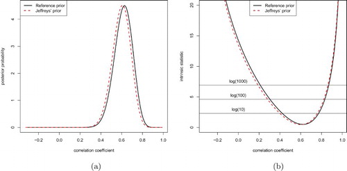
Table 4. The orthodontic data from Frees (2004).

	Age of girls				Age of boys
Number	8	10	12	14	8	10	12	14
1	21	20	21.5	23	26	25	29	31
2	21	21.5	24	25.5	21.5	22.5	23	26.5
3	20.5	24	24.5	26	23	22.5	24	27.5
4	23.5	24.5	25	26.5	25.5	27.5	26.5	27
5	21.5	23	22.5	23.5	20	23.5	22.5	26
6	20	21	21	22.5	24.5	25.5	27	28.5
7	21.5	22.5	23	25	22	22	24.5	26.5
8	23	23	23.5	24	24	21.5	24.5	25.5
9	20	21	22	21.5	23	20.5	31	26
10	16.5	19	19	19.5	27.5	28	31	31.5
11	24.5	25	28	28	23	23	23.5	25
12					21.5	23.5	24	28
13					17	24.5	26	29.5
14					22.5	25.5	25.5	26
15					23	24.5	26	30
16					22	21.5	23.5	25

Table 5. Estimations of ρ for the orthodontic data from Frees (2004).

Priors	Intrinsic	Mean	Median	Mode
	0.603	0.598	0.601	0.608
	0.622	0.616	0.620	0.627

On the other hand, the proposed solution can be used for the hypothesis testing of . If we are interested in testing , we can numerically verify that the intrinsic statistic under is which indicates that the expected value of the average of the log likelihood ratio against is about 14.2747, showing that the likelihood ratio is expected to be about 1,582,791. Thus we may conclude that the data provide very strong evidence against and that the null hypothesis is opposed to the observable data. Due to the invariance property of the proposed solution, if the parameter of interest is , then its intrinsic estimator is simply , and the corresponding non-rejection regions are simply given by , and , respectively.

5. Concluding remarks

In this paper, we first derived two objective priors for the unknown parameters in the intraclass model in (1(1) ) and proved that both result in proper posterior distributions. Within a Bayesian decision-theoretic framework, we then proposed an objective Bayesian solution to both hypothesis testing and point estimation problems of the ICC ρ. The proposed solution has an appealing invariance property under one-to-one reparametrisation of the quantity of interest, which is not shared by some commonly used estimators, such as the posterior mean.

It deserves mentioning that the proposed solution can be directly applied to the balanced one-way random effect ANOVA model, since it is a special case of the intraclass model in (1(1) ) if we let and , where and stand for the treatment and error variances, respectively. This observation motivates a possible extension of the proposed solution to the unbalanced model with different number of observations in each class, which is currently under investigation and will be reported elsewhere.

Acknowledgements

The authors thank the editor, an associate editor and one referee for their detailed and constructive comments, which have led to a significant improvement of the manuscript. This work was based on the first author's dissertation research which was supervised by the corresponding author. MW and DZ initiated and carried out the study. MW and DZ drafted the manuscript. DH, TL, and XS participated in the discussion and proofread the manuscript. All authors read and approved the final manuscript.

Disclosure statement

No potential conflict of interest was reported by the authors.

ORCID

Duo Zhang http://orcid.org/0000-0002-0249-1849

Min Wang http://orcid.org/0000-0002-9233-7844

Appendix

In the appendix, we prove that the posterior distribution is proper under in (5(5) ), since the case for is exactly the same and thus omitted for simplicity. We first provide a very useful lemma, which plays an important role in determining the tail behaviour of the key terms of the marginal posterior distribution .

Lemma .1

The marginal posterior distribution in (6(6) ) is a continuous function in and their terms are such that and as and such that and as

Proof.

Direct inspection shows that in (6(6) ) is a continuous function in . We consider the behaviour of its two key terms as (i) and (ii)

1. Let , which tends to infinity as . Given that , we have Then it follows that (A1) As , we have which show that , and thus In addition, as , we observe that each element of the inverse matrix in the right hand of Equation (A2(A2) ) becomes . With a little abuse of notation, as , we denote which shows that Note also that , where as . Also, Thus, as , it follows

2. Let , which tends to infinity as . Given that it follows that (A2) As , we have , and thus In addition, as , we observe that and that , where As , we have , and thus

Proof of Theorem 2.1.

Proof of Theorem 2.1

We now show that the posterior distribution under is proper. Recall that the corresponding marginal posterior of ρ is given by (A3) Then the reference prior leads to a proper posterior distribution if and only if By following Lemma A.1, we observe that , the tail behaviour of follows and that , the tail behaviour of follows Given that is a continuous function in , the posterior distribution under is proper, provided that . This completed the proof of Theorem 2.1.

Proof of Theorem 3.1.

Proof of Theorem 3.1

Define and . It can be easily verified that where represents the trace of the matrix .

Consider that the KL divergence measure of a normal linear model from another normal linear model is given by where . The minimum of the logarithmic divergence above for and is achieved when and substitution yields which is the same as in (9(9) ).

Similarly, the minimum of the logarithmic divergence measure of from is given by where . The minimum of the divergence measure above for and is achieved when and substitution yields Therefore, the intrinsic statistic is given by It can be easily shown that if and only if . This completed the proof of Theorem 3.1.

References

- Barkto, J. (1966). The intraclass correlation coefficient as a measure of reliability. Psychological Reports, 19, 2–11.
- Berger, J. O., & Bernardo, J. M. (1992a). On the development of reference priors. In J. M. Bernardo, J. O. Berger, A. P. Dawid, & A. F. M. Smith (Eds.), Bayesian statistics, 4 (Peñíscola, 1991) (pp. 35–60). New York: Oxford University Press.
- Berger, J. O., & Bernardo, J. M. (1992b). Reference priors in a variance components problem. In P. K. Goel & N. Sreenivas Iyengar (Eds.), Lecture notes in statistics: Vol. 75. Bayesian analysis in statistics and econometrics (Bangalore, 1988) (pp. 177–194). New York: Springer.
- Bernardo, J. (2010). Integrated objective Bayesian estimation and hypothesis testing. In J. M. Bernardo, M. J. Bayarri, J. O. Berger, A. P. Dawid, D. Heckerman, A. F. M. Smith, & M. West (Eds.), Bayesian statistics, 9. Proceedings of the ninth valencia international meeting (pp. 1–68). New York: Oxford University Press.
- Bernardo, J. M. (1979). Reference posterior distributions for Bayesian inference. Journal of the Royal Statistical Society. Series B (Methodological), 41, 113–147.
- Bernardo, J. M. (1999). Nested hypothesis testing: The Bayesian reference criterion. In J. M. Bernardo, J. O. Berger, A. P. Dawid, & A. F. M. Smith (Eds.), Bayesian statistics, 6 (Alcoceber, 1998) (pp. 101–130). New York: Oxford University Press.
- Bernardo, J. M. (2005). Reference analysis. In D. K. Dey & C. R. Rao (Eds.), Handbook of Statistics: Vol. 25. Bayesian thinking: Modeling and computation (pp. 17–90). Amsterdam: Elsevier/North-Holland.
- Bernardo, J. M., & Juárez, M. A. (2003). Intrinsic estimation. In J. M. Bernardo, M. J. Bayarri, J. O. Berger, A. P. Dawid, D. Heckerman, A. F. M. Smith, & M. West (Eds.), Bayesian statistics, 7 (Tenerife, 2002) (pp. 465–476). New York: Oxford University Press.
- Bernardo, J. M., & Pérez, S. (2007). Comparing normal means: New methods for an old problem. Bayesian Analysis, 2, 45–58. doi: 10.1214/07-BA202
- Bernardo, J. M., & Rueda, R. (2002). Bayesian hypothesis testing: A reference approach. International Statistical Review, 70, 351–372. doi: 10.1111/j.1751-5823.2002.tb00175.x
- Bernardo, J. M., & Smith, A. F. (1994). Bayesian theory. Chichester: Wiley.
- Box, G. E. P., & Tiao, G. C. (1973). Bayesian inference in statistical analysis. Reading, MA: Addison-Wesley.
- Chung, Y., & Dey, D. K. (1998). Bayesian approach to estimation of intraclass correlation using reference prior. Communications in Statistics: Theory and Methods, 27, 2241–2255. doi: 10.1080/03610929808832225
- Datta, G. S., & Ghosh, J. K. (1995a). Noninformative priors for maximal invariant parameter in group models. TEST, 4, 95–114. doi: 10.1007/BF02563105
- Datta, G. S., & Ghosh, J. K. (1995b). On priors providing frequentist validity for Bayesian inference. Biometrika, 82, 37–45. doi: 10.2307/2337625
- Datta, G. S., & Mukerjee, R. (2004). Probability matching priors: Higher order asymptotics. Lecture notes in statistics: Vol. 178. New York: Springer-Verlag.
- Fleiss, J. (1986). The design and analysis of clinical experiments. New York: Wiley.
- Frees, E. W. (2004). Longitudinal and panel data: Analysis and applications in the social sciences. New York: Cambridge University Press.
- Ghosh, M., & Heo, J. (2003). Noninformative priors, credible sets and Bayesian hypothesis testing for the intraclass model. Journal of Statistical Planning and Inference, 112, 133–146. doi: 10.1016/S0378-3758(02)00328-2
- Jelenkowska, T. H. (1998). Bayesian estimation of the intraclass correlation coefficients in the mixed linear model. Applications of Mathematics, 43, 103–110. doi: 10.1023/A:1023210900467
- Lin, L., Hedayat, A. S., Sinha, B., & Yang, M. (2002). Statistical methods in assessing agreement: Models, issues, and tools. Journal of the American Statistical Association, 97, 257–270. doi: 10.1198/016214502753479392
- Paul, S. R. (1990). Maximum likelihood estimation of intraclass correlation in the analysis of familial data: Estimating equation approach. Biometrika, 77, 549–555. doi: 10.1093/biomet/77.3.549
- Paul, S. R. (1996). Score tests for interclass correlation in familial data. Biometrics, 52, 955–963. doi: 10.2307/2533056
- Robert, C. P. (1996). Intrinsic losses. Theory and Decision, 40, 191–214. doi: 10.1007/BF00133173
- Sun, D., & Ye, K. (1996). Frequentist validity of posterior quantiles for a two-parameter exponential family. Biometrika, 83, 55–65. doi: 10.1093/biomet/83.1.55