
ABSTRACT
In this paper, we proposed a dynamic stress–strength model for coherent system. It is supposed that the system consists of n components with initial random strength and each component is subjected to random stresses. The stresses, applied repeatedly at random cycle times, will cause the degradation of strength. In addition, the number of cycles in an interval is assumed to follow a Poisson distribution. In the case of the strength and stress random variables following exponential distributions, the expression for the reliability of the proposed dynamic stress–strength model is derived based on survival signature. The reliability is estimated by using the best linear unbiased estimation (BLUE). Considering the Type-II censored failure times, the best linear unbiased predictors (BLUP) for the unobserved coherent system failure times are developed based on the observed failure times. Monte Carlo simulations are performed to compare the BLUE of parameters with different values and compute the BLUP. A real data set is also analysed for an illustration of the findings.
1. Introduction
Stress–strength model is of special importance in engineering applications. A technical system or component may be subjected to randomly occurring environmental stresses such as pressure, temperature, and humidity The survival of the system heavily depends on its resistance. In the simplest form of the stress–strength model, a failure occurs when the strength (or resistance) of the component drops below the stress. In this case the reliability R is defined as the probability that the component's strength is greater than the stress, that is, where X is the random strength of the component and Y is the random stress placed on it. The reliability has been widely studied under various distributional assumptions on X and Y (see, e.g. Johnson Citation1988; Kotz, Lumelskii, and Pensky Citation2003) Recently, Liu, Shi, and Bai (Citation2018) studied the estimation for the reliability of a N –M-cold-standby redundancy system based on progressive Type-II censoring sample. Chen and Cheng (Citation2017) discussed estimation of the system stress–strength reliability based on different point estimators and interval estimations when the underlying distribution was exponentiated Pareto distribution. Wang, Geng, and Zhou (Citation2018) developed inferential procedures for the generalised exponential stress–strength model based on generalised pivotal quantity. For more details on the SSR in recent years, see Khan and Jan (Citation2014), Kizilaslan and Nadar (Citation2015), Wang et al. (Citation2018), Rao, Rosaiah, and Babu (Citation2016), Mokhlis, Ibrahim, and Gharieb (Citation2017), Dey, Mazucheli, and Anis (Citation2017), Sales Filho, López Droguett, and Lins (Citation2017), and Baklizi (Citation2014).
In the aforementioned stress–strength model, stress and strength variables are considered to be static. Dynamic (time-dependent) stress–strength modelling may extend more realistic applications in real-life reliability studies than static modelling, which enables us to investigate the dynamic reliability properties of the system. In recent years, much attention has been paid to dynamic stress–strength modelling. Eryilmaz (Citation2013) studied the stress–strength reliability for the case in which the strength of the system is modelled as a stochastic process and the stress is considered to be a usual random variable. Bhuyan and Dewanji (Citation2017a), Bhuyan and Dewanji (Citation2017b), and Bhuyan, Mitra, and Dewanji (Citation2016) presented computation and estimation of reliability as well as identifiability issues under dynamic stress–strength modelling with deterministic strength degradation and cumulative damage due to shocks arriving according to a Poisson process. Cha and Finkelstein (Citation2015) considered a dynamic stress–strength modelling with decreasing strength with time and external shock (stress) process, such as Poisson process. A time-dependent stress–strength model with random strength and constant stresses which are repeatedly applied at random cycle times was researched by Siju and Kumar (Citation2016). However, there is little research about dynamic stress–strength modelling for multicomponent system among these literature.
In practice, it is meaningful to predict the unobserved failure times from current available observations for testing system. As mentioned in AL-Hussaini, Abdel-Hamid, and Hashem (Citation2015), to know about plausible warranty limits of products, the experimenters, manufacturers and customers would like to get the bounds of the products life. AL-Hussaini et al. (Citation2015) obtained Bayesian prediction intervals of unobserved progressively Type-II censored data in the presence of competing risks from half-logistic distribution. Basak, Basak, and Balakrishnan (Citation2006) predicted times to failure of censored units in progressively censored samples, including the best linear unbiased predictors (BLUP), the maximum likelihood predictors (MLP), and the conditional median predictors (CMP). Based on the good property of normal distribution, Basak and Balakrishnan (Citation2009) gave the BLUP, modified MLP, approximate MLP and CMP of normal failure times. Balakrishnan, Ng, and Navarro (Citation2011) discussed the BLUP of the Type-II censored (unobserved) system failure times based on the observed failures times. Basak (Citation2014) discussed the problem of predicting failure times for a simple step-stress model under regular and progressive Type-II censoring by computing the MLP and CMP. Asgharzadeh, Valiollahi, and Kundu (Citation2015) considered the classical point predictors and Bayesian predictors of Weibull failure times based on hybrid censored data.
The system signature has been found to be useful for comparisons the performance and quantification of the reliability of coherent system. A lucid review of the theory about signature and its application were presented by Samaniego (Citation2007). For a system with n components and lifetime the system signature is the vector
with component
where
stands for the ith smallest failure time among n components,
represents the probability that the system fails upon the failure of the ith component and
Hence, the well-known mixture representation for the survival function (SF) of the systems failure time is
(1) Referred to Eryilmaz (Citation2014) and Coolen Coolen-Maturi (Citation2013), Equation (Equation1
(1) ) can also be expressed as
(2) where
denotes the number of path sets of size k for the system,
denotes the number of components in the system that function at time t and
The vector
is called system survival signature. Compared to Samaniego's classical signature, the survival signature has the important advantage that it is applicable to system with multiple types of components. Coolen, Coolen-Maturi, and Al-nefaiee (Citation2013), Aslett, Coolen, and Wilson (Citation2015), and Coolen and Coolen-Maturi (Citation2016) dealt with reliability of systems and networks with multiple types of components based on the survival signature. Pakdaman, Ahmadi, and Doostparast (Citation2017) studied the stress–strength reliability based on survival signature. Except for that, there is little literature on the survival signature for stress–strength reliability of multicomponent systems, especially the dynamic stress–strength reliability (DSSR) of multicomponent systems.
This paper discusses the best linear unbiased estimation (BLUE) for coherent system DSSR with survival signature and the BLUP for unobserved coherent system failure times based on the observed failure times. We study the coherent system with n identical components. Each of these components with initial random strength X is subjected to random stress
which is repeatedly applied at random cycle times to cause the degradation of strength. Let the strength
on the ith cycle is given by
where c is a known constant and
The aforesaid coherent system has been widely applied in practical engineering fields. For example, a crane is assembled by many identical chains to lift heavier objects repeatedly of various sizes and weights (see Siju & Kumar, Citation2016).
The random strength of the chain is the bearing capacity and the repeated stresses are the weights of objects. The rest of this paper is organised as follows: In Section 2, the expression of the coherent system DSSR with survival signature is derived. Section 3 presents the exact expressions for the BLUE of the parameters, as well as their variances and covariances. The BLUP of unobserved coherent system failure times of the coherent systems are discussed in Section 4. In Section 5, a simulation study is performed to compare the estimations of parameters with different values, as well as compute the BLUP of the unobserved coherent system failure times by using Monte Carlo simulations and findings are illustrated by tables and figures. Furthermore, a real data set analysis is presented in Section 6. Finally, we conclude the paper in Section 7.
2. DSSR of the coherent system with survival signature
The goal of this section is to derive the expression of the coherent system DSSR with survival signature. In the following two subsections, the expressions of DSSR of the coherent system and its constituent component are obtained, respectively.
2.1. DSSR of the coherent system component
Let X and Y be independent random variables and distributed exponential distributions with different scale parameters and
respectively. The probability density functions (PDF), cumulative distribution functions (CDF) and SFs of X and Y can be expressed as
The scale parameters α and β can be readily estimated by the obtained samples of strength X and stress Y. Therefore, it is reasonable to suppose that α and β are known in this paper.
Suppose the stress Y =y is known and let be the event that no failure occurs on the ith cycle. The component reliability of success of the first i cycles can be given by
(3) If the stress Y is unknown, the component reliability of success of the first i cycles can be rewritten as
(4) Let
denote the number of cycles occurring in the time interval
Therefore,
is the point process and
denotes the probability that exact i cycles occur in time interval
Suppose that
is the Poisson process, then
(5) that is, the random variable
follows a Poisson distribution with parameter
This parameter is equal to the expected number of cycles in time interval
The Poisson process
with
has independent increments. Consequently, the component DSSR of the coherent system when
is given by
(6) where the random variable
implies the lifetime of the component with random initial strength X impacted by the random stress Y, and
implies the component static stress–strength reliability at t=0.
2.2. DSSR of the coherent system
Consider the coherent system with n identical components, which are mentioned in Section 2.1, acted upon by the stress
applied repeatedly at random times. Suppose the stress Y =y is known and the coherent system reliability of success of first i cycles by the use of survival signature
and Equation (Equation3
(3) ) is derived as
(7) where
and
denotes the number of path sets of size j for the coherent system. Define
can be rewritten as
(8) The vector
is called the minimal signature of the system (Balakrishnan et al., Citation2011). If the stress Y is unknown, the coherent system reliability of success of first i cycles can be rewritten as
(9) Let the random variable T be the lifetime of the coherent system. When
from Equation (Equation5
(5) ), the coherent system DSSR is expressed as
(10) Define
and
DSSR of the coherent system can be rewritten as
(11) Consequently, the CDF and PDF of T can be given by
(12)
(13) When
implies the static stress–strength reliability of coherent system.
3. Best linear unbiased estimation
Suppose m independent coherent systems with the same survival signature are placed on a life test. The test is terminated when the
(where
is pre-fixed) system fails. Additionally, the Type-II censored samples
of T are observed.
Denote the moments, the product moments, and the variance–covariance matrix of by
and
where
and
Define
and
The CDF and PDF of
can be expressed as
(14)
(15) Denote the moments, the product moments, and the variance–covariance matrix of
by
and
where
and
As a result, the moments and the variance–covariance matrix can be expressed as
(16)
(17) Define the generalised variance as
(18) According to Balakrishnan et al. (Citation2011), by minimising Q with respect to λ, the BLUE
of λ and its variance can be obtained as
(19)
(20) where
is the coefficient vector of the censored samples
To compute
the expressions of the moments
and variance–covariance matrix
will be given in the following two subsections.
3.1. Moments  of
of
On the basis of Equations (Equation14(14) )–(Equation15
(15) ), the PDF of
is derived as
(21) As a consequence, the expectation of
can be given by
(22) In addition, the values of
can be obtained by the use of triangle rule (see Theorem 5.3.1 in Arnold, Balakrishnan, & Nagaraja, Citation2008),
(23) where
Based on Equation (Equation23(23) ), it is readily to obtain that
where
Similarly, the values of
can be derived.
3.2. Variance–covariance matrix of
In order to obtain , we firstly compute the product moments
Since the symmetry of the variance–matrix
, we just need to compute
Case I: i=j,
Based on Equation (Equation21(21) ), the second moment of
can be obtained by
(24) Also, the values of
can be obtained by the use of triangle rule
where
Case II:
and
Consider the joint density of for
given by
(25) In the light of Equations (Equation14
(14) )–(Equation15
(15) ), the joint density function of
can be rewritten as
Define
and
then
(26) Moreover, define
Therefore, the product moment of
can be expressed as
(27) Based on Equation (Equation27
(27) ), the values of
can be readily obtained. And then, all other product moments can be computed by the use of rectangle rule (see Theorem 5.3.9 in Arnold et al., Citation2008)
(28) where
Hence, according to
the variance–covariance matrix
can be readily calculated.
4. Best linear unbiased predictors
According to Balakrishnan et al. (Citation2011), the BLUP of the Type-II censored (unobserved) coherent system failure times based on the observed failure times are discussed in this section.
From Equation (Equation19(19) ), the BLUE of the parameter λ based on the first r observed failure times can be rewritten as
(29) Then, from the results of Doganaksoy and Balakrishnan (Citation1997), by equating
the BLUP of
can be obtained as
(30) where
The predictor of
can be obtained in a similar manner by regarding the BLUP of
as observed failure times in the BLUE. Finally, the BLUP of
and its variance based on the first r failure times can be computed as
(31)
(32) where
can be calculated by equating
5. Numerical simulation
To study the performance of the BLUE of λ and BLUP of the Type-II censored (unobserved) coherent system failure times based on the observed failures times mentioned in the preceding sections, an extensive Monte Carlo simulation study is carried out in this section.
Six different coherent systems with different system signatures and structure, listed in Table , are considered. It is supposed that these systems are made up of the same components, which are mentioned in Section 2 with known parameters which are fixed by
and
The coefficients and
for these different coherent systems with different censored schemes are computed and the results are presented in Tables .
Table 1. The description of six different coherent systems.
Table 2. Coefficients of and corresponding for System 1.
Table 3. Coefficients of and corresponding for System 2.
Table 4. Coefficients of and corresponding for System 3.
Table 5. Coefficients of and corresponding for System 4.
Table 6. Coefficients of and corresponding for System 5.
Table 7. Coefficients of and corresponding for System 6.
Set the parameter respectively. For each value of the parameter, the Type-II censored samples of different censored schemes are generated. The BLUE
and standard error
are computed based on the coefficients in Tables . Repeat this process 10,000 times. The results are presented in Tables .
Table 8. BLUE and standard errors for 6 different coherent systems ().
Table 9. BLUE and standard errors for 6 different coherent systems ().
Table 10. BLUE and standard errors for six different coherent systems ().
Table 11. BLUE and standard errors for six different coherent systems ().
Additionally, for each coherent system, we generate the complete samples of the system by fixing and
Let
The predictors and corresponding variances
(
) for the Type-II censored (unobserved) coherent systems failure times based on the observed failures times are computed by using the first r samples. The results are presented in Table and the comparison of the predictors and the last m−r samples, as well as the variation of V are shown in Figure .
Figure 1. Comparison of the BLUP and samples and variation of variances.
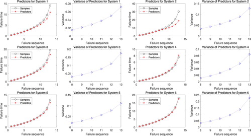
Table 12. BLUP and variances for six different coherent systems ().
From Tables , for each coherent system, it is readily seen that SE decreases as r increases, when m is fixed. SE decreases as m increases, when r is fixed. The deviation between the BLUE and fixed value of parameter λ reaches minimum when
where
is the top integral function. Additionally, the larger the fixed value of parameter λ, the greater the variance.
From Table and Figure , for each coherent system, it is observed that the predictors are closed to the real value of samples and V increases as i increases.
6. Real data analysis
In this section, a real data set in Lawless (Citation2011) is analysed by using the proposed methods. The data set represents failure times, in minutes, for two types of electrical insulation in an experiment in which the insulation is subjected to a continuously increasing voltage stress. 12 electrical insulations of each type are tested and recorded. The failure times of the first type are 12.3, 21.8, 24.4, 28.6, 43.2, 46.9, 70.7, 75.3, 95.5, 98.1, 138.6 and 151.9, while the failure times of the second type
are 18.5, 21.7, 35.1, 40.5, 42.3, 48.7, 79.4, 86.0, 121.9, 147.1, 150.2 and 219.3.
Let and
denote the failure times of two different coherent systems. It is assumed that the failure data
and
are from System 1 and System 3, respectively. Fix
and
Based on Equation (Equation12
(12) ), the CDFs of
and
can be expressed as
and
where
and
Using the proposed method in Section 3 and fixing
the BLUE of
for
and
for
can be computed, respectively. The Kolmogorov–Smirnov (K–S) test statistic and corresponding p-values are computed by using
and
The BLUEs of
and
K–S distances between the empirical distribution functions and the fitted distribution functions and corresponding p-values are presented in Table . Then, based on the K–S distances and p-values, one cannot reject the hypothesis that the data are coming from the above distributions.
Table 13. BLUE, K–S distance, and p-values of and based on data set.
For illustrative purpose, let and
It is supposed that
are the observed failure times for System 1 and
are the observed failure times for System 3. According to the proposed method in Section 4, the predictors
and
of the Type-II censored (unobserved) system failure times for System 1 and System 3 can be computed, respectively. For each coherent system, the predictors and corresponding variance V are presented in Table , as well as the comparisons of the predictors and the last m−r samples are shown in Figure .
Figure 2. Comparison of the BLUP and real data samples.
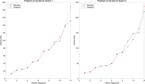
Table 14. BLUP and variances for real data analysis().
7. Conclusion
In this paper, we study the BLUE for dynamic stress–strength reliability of coherent systems, which consist of multiple identical components with random strength and are subjected to repeated random stresses at random cycle times, with survival signature. In addition, the BLUP for the Type-II censored coherent (unobserved) system failure times based on the observed failure times are discussed. According to the results of numerical simulation, it is readily seen that the larger the sample size, the more accurate the estimation. The failure number may minimise the deviation between the BLUE and parameter λ. In addition, the BLUP has a good performance.
Disclosure statement
No potential conflict of interest was reported by the authors.
Additional information
Funding
Notes on contributors
Yiming Liu
Yiming Liu is a PhD Candidate in the Department of Applied Mathematics, Northwestern Polytechnical University (P.R.China), and Yiming Liu’s supervisor is Prof. Yimin Shi. Yiming Liu is mainly engaged in system stress–strength reliability research.
Yimin Shi
Yimin Shi is a professor in the Department of Applied Mathematics, Northwestern Polytechnical University.
Xuchao Bai
Xuchao Bai is a Ph.D. Candidate in the Department of Applied Mathematics, Northwestern Polytechnical University (P.R.China), and his supervisor is Prof. Yimin Shi. He is working on life reliability and stress–strength reliability.
Bin Liu
Bin Liu is an associate professor in the Department of Applied Mathematics, Taiyuan University of Science and Science and Technology. Bin Liu is working on life reliability and stress–strength reliability.
References
- AL-Hussaini, E. K., Abdel-Hamid, A. H., & Hashem, A. F. (2015). Bayesian prediction intervals of order statistics based on progressively type-II censored competing risks data from the half-logistic distribution. Journal of the Egyptian Mathematical Society, 23(1), 190–196. doi: 10.1016/j.joems.2014.01.008
- Arnold, B. C., Balakrishnan, N., & Nagaraja, H. N. (2008). A first course in order statistics. Siam: Society for Industrial and Applied Mathematics.
- Asgharzadeh, A., Valiollahi, R., & Kundu, D. (2015). Prediction for future failures in Weibull distribution under hybrid censoring. Journal of Statistical Computation and Simulation, 85(4), 824–838. doi: 10.1080/00949655.2013.848451
- Aslett, L. J. M., Coolen, F., & Wilson, S. P. (2015). Bayesian inference for reliability of systems and networks using the survival signature. Risk Analysis, 35(9), 1640–1651. doi: 10.1111/risa.12228
- Baklizi, A. (2014). Interval estimation of the stress–strength reliability in the two-parameter exponential distribution based on records. Journal of Statistical Computation and Simulation, 84(12), 2670–2679. doi: 10.1080/00949655.2013.816307
- Balakrishnan, N., Ng, H. K. T., & Navarro, J. (2011). Linear inference for type-II censored lifetime data of reliability systems with known signatures. IEEE Transactions on Reliability, 60(2), 426–440. doi: 10.1109/TR.2011.2134371
- Basak, I. (2014). Prediction of times to failure of censored items for a simple step-stress model with regular and progressive type I censoring from the exponential distribution. Communications in Statistics – Theory and Methods, 43(10–12), 2322–2341. doi: 10.1080/03610926.2013.861489
- Basak, I., & Balakrishnan, N. (2009). Predictors of failure times of censored units in progressively censored samples from normal distribution. Sankhyā: The Indian Journal of Statistics, Series B (2008-), 71(2), 222–247.
- Basak, I., Basak, P., & Balakrishnan, N. (2006). On some predictors of times to failure of censored items in progressively censored samples. Computational Statistics & Data Analysis, 50(5), 1313–1337. doi: 10.1016/j.csda.2005.01.011
- Bhuyan, P., & Dewanji, A. (2017a). Reliability computation under dynamic stress–strength modeling with cumulative stress and strength degradation. Communications in Statistics-Simulation and Computation, 46(4), 2701–2713. doi: 10.1080/03610918.2015.1057288
- Bhuyan, P., & Dewanji, A. (2017b). Estimation of reliability with cumulative stress and strength degradation. Statistics, 51(4), 766–781. doi: 10.1080/02331888.2016.1277224
- Bhuyan, P., Mitra, M., & Dewanji, A. (2016). Identifiability issues in dynamic stress–strength modeling. Annals of the Institute of Statistical Mathematics, 70(1), 63–81. doi: 10.1007/s10463-016-0579-4
- Cha, J. H., & Finkelstein, M. (2015). A dynamic stress–strength model with stochastically decreasing strength. Metrika, 78(7), 807–827. doi: 10.1007/s00184-015-0528-x
- Chen, J., & Cheng, C. (2017). Reliability of stress–strength model for exponentiated Pareto distributions. Journal of Statistical Computation and Simulation, 87(4), 791–805. doi: 10.1080/00949655.2016.1226309
- Coolen, F. P. A., & Coolen-Maturi, T. (2013). Generalizing the signature to systems with multiple types of components. Complex Systems and Dependability, 170, 115–130. doi: 10.1007/978-3-642-30662-4_8
- Coolen, F. P. A., & Coolen-Maturi, T. (2016). On the structure function and survival signature for system reliability. Safety and Reliability, 36(2), 77–87. doi: 10.1080/09617353.2016.1219936
- Coolen, F. P. A., Coolen-Maturi, T., & Al-nefaiee, A. H. (2013). Recent advances in system reliability using the survival signature. Proceedings advances in risk and reliability technology symposium (pp. 205–217). Loughborough.
- Dey, S., Mazucheli, J., & Anis, M. Z. (2017). Estimation of reliability of multicomponent stress–strength for a Kumaraswamy distribution. Communications in Statistics – Theory and Methods, 46(4), 1560–1572. doi: 10.1080/03610926.2015.1022457
- Doganaksoy, N., & Balakrishnan, N. (1997). A useful property of best linear unbiased predictors with applications to life-testing. The American Statistician, 51(1), 22–28.
- Eryilmaz, S. (2013). On stress–strength reliability with a time-dependent strength. Journal of Quality and Reliability Engineering, 2013, 1–6. doi: 10.1155/2013/417818
- Eryilmaz, S. (2014). Computing reliability indices of repairable systems via signature. Journal of Computational and Applied Mathematics, 260, 229–235. doi: 10.1016/j.cam.2013.09.023
- Johnson, R. A. (1988). Stress–strength models for reliability. Handbook of Statistics, 7(88), 27–54. doi: 10.1016/S0169-7161(88)07005-1
- Khan, A. H., & Jan, T. R. (2014). Estimation of multi component systems reliability in stress–strength models. Journal of Modern Applied Statistical Methods, 13(2), 389–398. doi: 10.22237/jmasm/1414815600
- Kizilaslan, F., & Nadar, M. (2015). Classical and Bayesian estimation of reliability in multicomponent stress–strength model based on Weibull distribution. Revista Colombiana de Estadística, 38(2), 467–484. doi: 10.15446/rce.v38n2.51674
- Kotz, S., Lumelskii, Y., & Pensky, M. (2003). The stress–strength model and its generalizations: Theory and applications. Singapore: World Scientific.
- Lawless, J. F. (2011). Statistical models and methods for lifetime data. Hoboken: John Wiley & Sons.
- Liu, Y., Shi, Y., & Bai, X. (2018). Reliability estimation of a N-M-cold-standby redundancy system in a multicomponent stress–strength model with generalized half-logistic distribution. Physica A: Statistical Mechanics and its Applications, 490, 231–249. doi: 10.1016/j.physa.2017.08.028
- Mokhlis, N. A., Ibrahim, E. J., & Gharieb, D. M. (2017). Stress–strength reliability with general form distributions. Communications in Statistics – Theory and Methods, 46(3), 1230–1246. doi: 10.1080/03610926.2015.1014110
- Pakdaman, Z., Ahmadi, J., & Doostparast, M. (2017). Signature-based approach for stress–strength systems. Statistical Papers, 1–17. doi: 10.1007/s00362-017-0889-5
- Rao, G. S., Rosaiah, K., & Babu, M. S. (2016). Estimation of stress–strength reliability from exponentiated Fréchet distribution. The International Journal of Advanced Manufacturing Technology, 86(9–12), 3041–3049. doi: 10.1007/s00170-016-8404-z
- Sales Filho, R. L. M., López Droguett, E., & Lins, I. D. (2017). Stress–strength reliability analysis with extreme values based on q-exponential distribution. Quality and Reliability Engineering International, 33(3), 457–477. doi: 10.1002/qre.2020
- Samaniego, F. J. (2007). System signatures and their applications in engineering reliability. Davis: Springer Science & Business Media.
- Siju, K. C., & Kumar, M. (2016). Reliability analysis of time dependent stress–strength model with random cycle times. Perspectives in Science, 8, 654–657. doi: 10.1016/j.pisc.2016.06.049
- Wang, B. X., Geng, Y., & Zhou, J. X. (2018). Inference for the generalized exponential stress–strength model. Applied Mathematical Modelling, 53, 267–275. doi: 10.1016/j.apm.2017.09.012