Shape-constrained semiparametric additive stochastic volatility models

ABSTRACT

Nonparametric stochastic volatility models, although providing great flexibility for modelling the volatility equation, often fail to account for useful shape information. For example, a model may not use the knowledge that the autoregressive component of the volatility equation is monotonically increasing as the lagged volatility increases. We propose a class of additive stochastic volatility models that allow for different shape constraints and can incorporate the leverage effect – asymmetric impact of positive and negative return shocks on volatilities. We develop a Bayesian fitting algorithm and demonstrate model performance on simulated and empirical datasets. Unlike general nonparametric models, our model sacrifices little when the true volatility equation is linear. In nonlinear situations we improve the model fit and the ability to estimate volatilities over general, unconstrained, nonparametric models.

KEYWORDS:

• Bayesian isotonic regression
• leverage effect
• Markov chain Monte Carlo
• nonlinear time series
• particle filter
• state space model

1. Introduction

In financial econometrics, volatility is usually defined as the conditional standard deviation of a discrete-time return series $\{r_t,t\in \mathbb{Z}\}$; namely, ${\sigma }_t=\sqrt{\mathrm{Var}\left(r_t|{\mathcal{F}}_{t-1}\right)}$ where ${\mathcal{F}}_{t-1}$ is the filtration up to time t−1. Since Engle (1982)'s pioneering autoregressive conditional heteroscedastic (ARCH) model, a plethora of parametric models have been proposed to model financial volatilities. A popular approach is the stochastic volatility (SV) model that originated from Hull and White (1987)'s stochastic differential equation for option pricing. In volatility modelling, two functional relationships are of particular interest – the dependence of volatilities on lagged volatilities, i.e., the autoregressive component, as well as the relationship between volatilities and lagged return shocks, which is also known as the news impact curve in the ARCH literature (see, e.g., Engle & Gonzalez-Rivera, 1991; Engle & Ng, 1993). The basic discrete-time SV model (Taylor, 1994) is essentially a nonlinear state space model with the state variables, the log volatilities, following an autoregressive (AR) process. To capture the asymmetric impact of positive and negative return shocks on volatilities in SV models, researchers have introduced the ‘leverage effect’. A leverage effect is defined as a (usually negative) correlation between the innovations of the volatility process and the lagged innovations of the return process (see Harvey & Shephard, 1996; Yu, 2005). When the error distributions in the SV models (see Section 2) are normal, the leverage effect can be equivalently expressed as a linear function of the lagged return innovations in the volatility equation (see, e.g., Omori, Chib, Shephard, & Nakajima, 2007; Yu, 2005, 2012).

Although parametric assumptions in traditional SV models, such as the linearity of the autoregressive and leverage components, provide reasonable approximations in some settings, they can also deviate considerably from the truth. Comte (2004) showed the nonlinearity of the autoregressive component in SV models for large cap indices of several major equity markets. Yu (2012) found empirical evidence that the leverage effect for many U.S. large cap equity returns is significantly smaller than zero when the lagged return innovation is negative but not when it is positive, which implies that a linear leverage function is insufficient to capture the news impact curve.

Nonparametric or semiparametric SV models can be used to relax the linearity assumptions in traditional SV models. Such models offer great flexibility for modelling the nonlinear functional relationships in the volatility equation. However, due to the latent structure of the state space model, they can also lead to a very large estimation variance for the volatilities. In this article, we propose to incorporate our knowledge about the shapes (such as monotonicity or piecewise monotonicity) of the functional components in the volatility equation as additional constraints in semiparametric SV models. In particular, we implement the shape constraints in the prior distributions of our Bayesian semiparametric additive model and show that the resulting model is more flexible than the linear parametric model and that the shape-constrained model can achieve lower estimation errors of the log volatilities and higher predictive log likelihood compared to the semiparametric model without shape constraints.

The idea of imposing shape constraints in a semiparametric SV model is warranted by the availability of our knowledge about the functional shapes as well as the proven benefits of imposing shape constraints in linear and generalised linear models. The past two decades have witnessed the accumulation of significant empirical knowledge about the shapes of the autoregressive and leverage components in SV models. For example, the phenomenon of volatility clustering (e.g., Rydberg, 2000) suggests that the autoregressive component of the volatility equation should be monotonically increasing as the lagged volatility increases. Additionally, Yu (2012)'s findings show that the leverage function should at least be monotonically decreasing on the negative real line. Additionally, it has long been established that imposing correct shape constraints in function estimation problems has the potential of greatly improving model fit without incurring much additional cost (Ramsay, 1988). As a result, shape-constrained function estimation has been widely applied in regression and generalised linear models (for Bayesian implementations, see Brezger & Steiner, 2008; Cai & Dunson, 2007; Meyer, Hackstadt, & Hoeting, 2011; Neelon & Dunson, 2004). In state-space models such as SV models, there has been, to the best of our knowledge, no demonstration of the benefits of shape-constrained state smoothing. It is our belief that the aforementioned functional shapes shall be exploited to provide additional regularisation in the semiparametric SV models to ensure better model fit and prediction accuracy.

The remainder of the article is organised as follows. In Section 2, we introduce our shape-constrained semiparametric additive SV model. In Section 3, we develop the Markov chain Monte Carlo procedures for sampling from the posterior distribution and a particle-filter-based procedure for evaluating the predictive log likelihood. We apply our methods to simulated and real-world financial returns in Sections 4 and 5 and demonstrate their advantages over both the linear SV model and the semiparametric model without shape constraints. We close with conclusions and discussions in Section 6.

2. Model specification

2.1. Additive stochastic volatility models

The basic parametric (Gaussian) SV model is (1) $\begin{array}{rl}{r}_t& =\omega +\exp \left(h_t/2\right){\epsilon }_t,{\epsilon }_t\stackrel{\mathrm{iid}}{\sim }N(0,1);\\ h_t& =\mu +\phi h_{t-1}+{\eta }_{t-1},{\eta }_t\stackrel{\mathrm{iid}}{\sim }N(0,{\sigma }_1^2),\end{array}$(1) where $\{{\epsilon }_t{\}}_{t\in \mathbb{Z}}$ and $\{{\eta }_t{\}}_{t\in \mathbb{Z}}$ are two mutually independent innovation processes. To induce a leverage effect, we assume that $\mathrm{corr}({\epsilon }_{t-1},{\eta }_t)=\rho$. Since the error distributions are normal, the state equation of the leveraged SV model can be equivalently expressed as (2) $h_t=\mu +\phi h_{t-1}+\psi {\epsilon }_{t-1}+{\xi }_t,{\xi }_t\stackrel{\mathrm{iid}}{\sim }N(0,{\sigma }_2^2),$(2) where $\psi =\rho {\sigma }_1$, ${\sigma }_2={\sigma }_1\sqrt{1-{\rho }^2}$ and $\{{\epsilon }_t{\}}_{t\in \mathbb{Z}}$ is independent from $\{{\xi }_t{\}}_{t\in \mathbb{Z}}$. This alternative form of the leverage effect (2(2) $h_t=\mu +\phi h_{t-1}+\psi {\epsilon }_{t-1}+{\xi }_t,{\xi }_t\stackrel{\mathrm{iid}}{\sim }N(0,{\sigma }_2^2),$(2) ) has been exploited in several papers including (Omori et al., 2007; Yu, 2005, 2012).

In this article, we consider the following semiparametric stochastic volatility model: (3) $\begin{array}{rl}{r}_t& =\omega +\exp \left(h_t/2\right){\epsilon }_t,{\epsilon }_t\stackrel{\mathrm{iid}}{\sim }N(0,1);\\ h_t& =\mu +f\left(h_{t-1}\right)+g\left({\epsilon }_{t-1}\right)+{\xi }_t,{\xi }_t\stackrel{\mathrm{iid}}{\sim }N(0,{\sigma }^2),\end{array}$(3) where the innovations $\{{\epsilon }_t{\}}_{t\in \mathbb{Z}}$ and $\{{\xi }_t{\}}_{t\in \mathbb{Z}}$ are mutually independent. We assume that the autoregressive component, f, and the leverage function, g, are additive. The leveraged SV model (2(2) $h_t=\mu +\phi h_{t-1}+\psi {\epsilon }_{t-1}+{\xi }_t,{\xi }_t\stackrel{\mathrm{iid}}{\sim }N(0,{\sigma }_2^2),$(2) ) is a special case of (3(3) $\begin{array}{rl}{r}_t& =\omega +\exp \left(h_t/2\right){\epsilon }_t,{\epsilon }_t\stackrel{\mathrm{iid}}{\sim }N(0,1);\\ h_t& =\mu +f\left(h_{t-1}\right)+g\left({\epsilon }_{t-1}\right)+{\xi }_t,{\xi }_t\stackrel{\mathrm{iid}}{\sim }N(0,{\sigma }^2),\end{array}$(3) ) when both f and g are linear functions. Model (3(3) $\begin{array}{rl}{r}_t& =\omega +\exp \left(h_t/2\right){\epsilon }_t,{\epsilon }_t\stackrel{\mathrm{iid}}{\sim }N(0,1);\\ h_t& =\mu +f\left(h_{t-1}\right)+g\left({\epsilon }_{t-1}\right)+{\xi }_t,{\xi }_t\stackrel{\mathrm{iid}}{\sim }N(0,{\sigma }^2),\end{array}$(3) ) includes the models of Comte (2004) and Yu (2012) as special cases: when $g\left({\epsilon }_{t-1}\right)=0$, (3(3) $\begin{array}{rl}{r}_t& =\omega +\exp \left(h_t/2\right){\epsilon }_t,{\epsilon }_t\stackrel{\mathrm{iid}}{\sim }N(0,1);\\ h_t& =\mu +f\left(h_{t-1}\right)+g\left({\epsilon }_{t-1}\right)+{\xi }_t,{\xi }_t\stackrel{\mathrm{iid}}{\sim }N(0,{\sigma }^2),\end{array}$(3) ) reduces to Comte (2004)'s nonparametric unleveraged SV model; when f is linear and g is piecewise linear, (3(3) $\begin{array}{rl}{r}_t& =\omega +\exp \left(h_t/2\right){\epsilon }_t,{\epsilon }_t\stackrel{\mathrm{iid}}{\sim }N(0,1);\\ h_t& =\mu +f\left(h_{t-1}\right)+g\left({\epsilon }_{t-1}\right)+{\xi }_t,{\xi }_t\stackrel{\mathrm{iid}}{\sim }N(0,{\sigma }^2),\end{array}$(3) ) becomes Yu (2012)'s semiparametric leverage effect model. Additionally, when ${\xi }_t=0$ for all t, model (3(3) $\begin{array}{rl}{r}_t& =\omega +\exp \left(h_t/2\right){\epsilon }_t,{\epsilon }_t\stackrel{\mathrm{iid}}{\sim }N(0,1);\\ h_t& =\mu +f\left(h_{t-1}\right)+g\left({\epsilon }_{t-1}\right)+{\xi }_t,{\xi }_t\stackrel{\mathrm{iid}}{\sim }N(0,{\sigma }^2),\end{array}$(3) ) contains the exponential ARCH (EGARCH) model of Nelson (1991).

Additional constraints on the functions f and g are needed for (3(3) $\begin{array}{rl}{r}_t& =\omega +\exp \left(h_t/2\right){\epsilon }_t,{\epsilon }_t\stackrel{\mathrm{iid}}{\sim }N(0,1);\\ h_t& =\mu +f\left(h_{t-1}\right)+g\left({\epsilon }_{t-1}\right)+{\xi }_t,{\xi }_t\stackrel{\mathrm{iid}}{\sim }N(0,{\sigma }^2),\end{array}$(3) ) to be identifiable. We assume that $f\left(h_m\right)=0$ and $g\left({\epsilon }_m\right)=0$, where $h_m$ and ${\epsilon }_m$ are two fixed numbers within the respective ranges of the processes $\{h_t{\}}_{t\in \mathbb{Z}}$ and $\{{\epsilon }_t{\}}_{t\in \mathbb{Z}}$. Under these conditions, the parameter μ in (3(3) $\begin{array}{rl}{r}_t& =\omega +\exp \left(h_t/2\right){\epsilon }_t,{\epsilon }_t\stackrel{\mathrm{iid}}{\sim }N(0,1);\\ h_t& =\mu +f\left(h_{t-1}\right)+g\left({\epsilon }_{t-1}\right)+{\xi }_t,{\xi }_t\stackrel{\mathrm{iid}}{\sim }N(0,{\sigma }^2),\end{array}$(3) ) represents the expected conditional log volatility when $h_{t-1}=h_m$ and ${\epsilon }_{t-1}={\epsilon }_m$. The choice of $h_m$ and ${\epsilon }_m$ is discussed in Section 2.2. For the remainder of the article, we will assume that the data have already been de-trended, so $\omega =0$.

2.2. Shape-constrained additive stochastic volatility models

We call model (3(3) $\begin{array}{rl}{r}_t& =\omega +\exp \left(h_t/2\right){\epsilon }_t,{\epsilon }_t\stackrel{\mathrm{iid}}{\sim }N(0,1);\\ h_t& =\mu +f\left(h_{t-1}\right)+g\left({\epsilon }_{t-1}\right)+{\xi }_t,{\xi }_t\stackrel{\mathrm{iid}}{\sim }N(0,{\sigma }^2),\end{array}$(3) ) the shape-constrained semiparametric additive SV model if f and g are restricted to be of certain shapes. As discussed in Section 1, for equity returns, the autoregressive function f is typically monotonically increasing on the entire real line, while the leverage function g is monotonically decreasing (at least) on the negative real line. The findings in Yu (2012) indicate that $g\left({\epsilon }_{t-1}\right)$ might have some change-point behaviour about zero, but generally, our knowledge of $g\left({\epsilon }_{t-1}\right)$ for positive ${\epsilon }_{t-1}$ is mixed.

To construct a monotone function $q\left(x\right)$, we consider the following basis expansion: (4) $q\left(x\right)={\beta }_0+{\beta }_1{w}_1\left(x\right)+\cdots +{\beta }_J{w}_J\left(x\right).$(4) If $w_j\left(x\right)$'s are monotonically increasing in x, then $q\left(x\right)$ is monotonically increasing (decreasing) in x if ${\beta }_j\ge (\le )$ 0 for all $j\ge 1$. In particular, given pre-specified knots ${\gamma }_0\le \cdots \le {\gamma }_J$, we propose the following basis functions (5) $\begin{array}{r}{w}_j\left(x\right)=\left\{\begin{array}{l}I(x>{\gamma }_{j-1})[min(x,{\gamma }_j)-{\gamma }_{j-1}]-({\gamma }_j-{\gamma }_{j-1})\\ \text{if }1\le j<M;\\ I(x>{\gamma }_{j-1})[min(x,{\gamma }_j)-{\gamma }_{j-1}]\\ \text{if }M\le j\le J,\end{array}\right.\end{array}$(5) where ${\gamma }_M$ denotes the ‘center’ of the range of x. As for the choice of M, when the argument of the function, x, represents the previous log volatility, $h_{t-1}$, we let $M=\lceil (J+1)/2\rceil$. When x represents the lagged return innovation, ${\epsilon }_{t-1}$, we can always include 0 as the knot ${\gamma }_{M-1}$.

The basis functions (5(5) $\begin{array}{r}{w}_j\left(x\right)=\left\{\begin{array}{l}I(x>{\gamma }_{j-1})[min(x,{\gamma }_j)-{\gamma }_{j-1}]-({\gamma }_j-{\gamma }_{j-1})\\ \text{if }1\le j<M;\\ I(x>{\gamma }_{j-1})[min(x,{\gamma }_j)-{\gamma }_{j-1}]\\ \text{if }M\le j\le J,\end{array}\right.\end{array}$(5) ) are a shifted version of the basis functions used in Neelon and Dunson (2004), but they considerably improve the computational efficiency for the class of state space models entertained in this article. Note that under (5(5) $\begin{array}{r}{w}_j\left(x\right)=\left\{\begin{array}{l}I(x>{\gamma }_{j-1})[min(x,{\gamma }_j)-{\gamma }_{j-1}]-({\gamma }_j-{\gamma }_{j-1})\\ \text{if }1\le j<M;\\ I(x>{\gamma }_{j-1})[min(x,{\gamma }_j)-{\gamma }_{j-1}]\\ \text{if }M\le j\le J,\end{array}\right.\end{array}$(5) ), the parameter ${\beta }_0$ in (4(4) $q\left(x\right)={\beta }_0+{\beta }_1{w}_1\left(x\right)+\cdots +{\beta }_J{w}_J\left(x\right).$(4) ) represents the ‘center’ of the function through the equation ${\beta }_0=q\left({\gamma }_{M-1}\right)$, while ${\beta }_0=q\left({\gamma }_0\right)$ under the original basis functions of Neelon and Dunson (2004). This makes a difference computationally since the basis functions are nonorthogonal (hence the coefficients are mutually dependent by design) and the estimation variance of $q\left({\gamma }_{M-1}\right)$ tends to be much smaller than that of $q\left({\gamma }_0\right)$ because of the abundance of information contributed by the data from both sides of ${\gamma }_{M-1}$. For SV models or other state space models, the benefits of the basis functions (5(5) $\begin{array}{r}{w}_j\left(x\right)=\left\{\begin{array}{l}I(x>{\gamma }_{j-1})[min(x,{\gamma }_j)-{\gamma }_{j-1}]-({\gamma }_j-{\gamma }_{j-1})\\ \text{if }1\le j<M;\\ I(x>{\gamma }_{j-1})[min(x,{\gamma }_j)-{\gamma }_{j-1}]\\ \text{if }M\le j\le J,\end{array}\right.\end{array}$(5) ) are even bigger due the necessity of specifying the knots with a wide enough range to cover all possible values of the latent variables and the resulting scarcity (or lack) of data for estimating $q\left({\gamma }_0\right)$.

Letting $w\left(h_{t-1}\right)$ and $v\left({\epsilon }_{t-1}\right)$ denote the basis functions for f and g respectively, we can rewrite (3(3) $\begin{array}{rl}{r}_t& =\omega +\exp \left(h_t/2\right){\epsilon }_t,{\epsilon }_t\stackrel{\mathrm{iid}}{\sim }N(0,1);\\ h_t& =\mu +f\left(h_{t-1}\right)+g\left({\epsilon }_{t-1}\right)+{\xi }_t,{\xi }_t\stackrel{\mathrm{iid}}{\sim }N(0,{\sigma }^2),\end{array}$(3) ) as (6) $\begin{array}{rl}{r}_t& =\exp \left(h_t/2\right){\epsilon }_t,{\epsilon }_t\stackrel{\mathrm{iid}}{\sim }N(0,1);\\ h_t& =\mu +\sum _{k=1}^K{\beta }_k{w}_k\left(h_{t-1}\right)+\sum _{l=1}^L{\alpha }_l{v}_l\left({\epsilon }_{t-1}\right)+{\xi }_t,\\ & {\xi }_t\stackrel{\mathrm{iid}}{\sim }N(0,{\sigma }^2).\end{array}$(6) It is easy to see that model (6(6) $\begin{array}{rl}{r}_t& =\exp \left(h_t/2\right){\epsilon }_t,{\epsilon }_t\stackrel{\mathrm{iid}}{\sim }N(0,1);\\ h_t& =\mu +\sum _{k=1}^K{\beta }_k{w}_k\left(h_{t-1}\right)+\sum _{l=1}^L{\alpha }_l{v}_l\left({\epsilon }_{t-1}\right)+{\xi }_t,\\ & {\xi }_t\stackrel{\mathrm{iid}}{\sim }N(0,{\sigma }^2).\end{array}$(6) ) satisfies $f\left({\gamma }_{M-1}^h\right)=\sum _{k=1}^K{\beta }_k{w}_k\left({\gamma }_{M-1}^h\right)=0$ and $g\left({\gamma }_{M-1}^{\epsilon }\right)=\sum _{l=1}^L{\alpha }_l{v}_l\left({\gamma }_{M-1}^{\epsilon }\right)=0$, which are the additional constraints needed for it to be identifiable. We use the following priors from Neelon and Dunson (2004) on $\{{\beta }_k{\}}_{k=1}^K$ to ensure their non-negativity: (7) $\begin{array}{rl}{\beta }_1^{\ast }& \sim \pi \left({\beta }_1^{\ast }\right);\\ {\beta }_k^{\ast }& \sim N({\beta }_{k-1}^{\ast },{\tau }^2),k\ge 2;\\ {\beta }_k& =I({\beta }_k^{\ast }>0){\beta }_k^{\ast },k\in \{1,\dots ,K\}.\end{array}$(7) The prior for ${\beta }_1^{\ast }$ can be based on prior knowledge of the steepness of the function toward the left tail. However, if such knowledge is not readily available, the flat prior $\pi \left({\beta }_1^{\ast }\right)\propto 1$ can be a convenient alternative, which also has a nice property that the posterior distribution does not depend on the starting point, nor on the direction of the latent random walk process $\{{\beta }_k^{\ast }{\}}_{k=1}^K$. In other words, the posterior will be exactly the same as by assuming the random walk starts at ${\beta }_{\kappa }^{\ast }$ with $\pi \left({\beta }_{\kappa }^{\ast }\right)\propto 1$, for any integer κ from 1 to K.

As for the function $g\left({\epsilon }_{t-1}\right)=\sum _l{\alpha }_l{v}_l\left({\epsilon }_{t-1}\right)$, we have empirical evidence showing that it is monotonically decreasing on the negative real line but do not have consistent information about its shape on the positive real line. Accordingly, our priors for $\{{\alpha }_l{\}}_{l=1}^L$ are specified as follows. (8) $\begin{array}{rl}{\alpha }_1^{\ast }& \sim \pi \left({\alpha }_1^{\ast }\right);\\ {\alpha }_l^{\ast }& \sim N({\alpha }_{l-1}^{\ast },{\gamma }^2),l\ge 2;\\ {\alpha }_l& =I({\alpha }_l^{\ast }<0){\alpha }_l^{\ast },l\le M-1;\end{array}$(8) (9) $\begin{array}{rl}{\alpha }_l& =\iota \left({\alpha }_l^{\ast }\right){\alpha }_l^{\ast },l\ge M.\end{array}$(9) In the equation above, $\pi \left({\alpha }_1^{\ast }\right)$ can be specified in the same way as $\pi \left({\beta }_1^{\ast }\right)$ and ι is an indicator function that depends on the assumption of the shape of g on the positive real line – if $g\left({\epsilon }_{t-1}\right)$ is monotonically decreasing in positive ${\epsilon }_{t-1}$, then $\iota \left({\alpha }_l^{\ast }\right)=I({\alpha }_l^{\ast }<0)$; if $g\left({\epsilon }_{t-1}\right)$ is monotonically increasing in positive ${\epsilon }_{t-1}$, then $\iota \left({\alpha }_l^{\ast }\right)=I({\alpha }_l^{\ast }>0)$; finally, if we lack such information or that $g\left({\epsilon }_{t-1}\right)$ is not monotone for positive ${\epsilon }_{t-1}$, we can simply set $\iota \left({\alpha }_l^{\ast }\right)=1$ to remove the shape constraint on that part of the leverage function altogether.

The remaining parameters are assumed to be mutually independent. For the priors of the variance parameters ${\sigma }^2,{\tau }^2$ and ${\gamma }^2$, we use the conjugate inverse gamma distribution. We assume a $N(0,d_{\mu }^2)$ prior for μ and a $N(0,d_0^2)$ prior for the initial state $h_1$.

3. Model fitting and comparison

3.1. MCMC procedure

We use the Gibbs sampler to simulate from the joint posterior distribution of model (6(6) $\begin{array}{rl}{r}_t& =\exp \left(h_t/2\right){\epsilon }_t,{\epsilon }_t\stackrel{\mathrm{iid}}{\sim }N(0,1);\\ h_t& =\mu +\sum _{k=1}^K{\beta }_k{w}_k\left(h_{t-1}\right)+\sum _{l=1}^L{\alpha }_l{v}_l\left({\epsilon }_{t-1}\right)+{\xi }_t,\\ & {\xi }_t\stackrel{\mathrm{iid}}{\sim }N(0,{\sigma }^2).\end{array}$(6) ). The algorithm for a single iteration is described below.

1. Update $\{{\beta }_k^{\ast }{\}}_{k=1}^K$ and $\{{\alpha }_l^{\ast }{\}}_{l=1}^L$ sequentially from their full conditional distributions, which are mixtures of two truncated normal distributions for the shape-constrained semiparametric model and normal for the corresponding semiparametric model without shape constraints. See the appendix for more details. For the shape-constrained model, compute $\{{\beta }_k{\}}_{k=1}^K$ and $\{{\alpha }_l{\}}_{l=1}^L$ deterministically using (7(7) $\begin{array}{rl}{\beta }_1^{\ast }& \sim \pi \left({\beta }_1^{\ast }\right);\\ {\beta }_k^{\ast }& \sim N({\beta }_{k-1}^{\ast },{\tau }^2),k\ge 2;\\ {\beta }_k& =I({\beta }_k^{\ast }>0){\beta }_k^{\ast },k\in \{1,\dots ,K\}.\end{array}$(7) )–(9(9) $\begin{array}{rl}{\alpha }_l& =\iota \left({\alpha }_l^{\ast }\right){\alpha }_l^{\ast },l\ge M.\end{array}$(9) ).

2. Update the variance parameters ${\tau }^2,{\gamma }^2$ and ${\sigma }^2$ from their inverse gamma full conditional distributions.

3. Update μ from its normal full conditional distribution.

4. Update $\{h_t,t=1,\dots ,T\}$ sequentially from their full conditional distributions using the random-walk Metropolis-Hastings algorithm.

One challenge of this MCMC algorithm is that both the ‘dependent variable’, $h_t$, and the ‘independent variables’, $h_{t-1}$ and ${\epsilon }_{t-1}$, of the state equation change from iteration to iteration. Therefore, in order to update the coefficients $\{{\beta }_k{\}}_{k=1}^K$ and $\{{\alpha }_l{\}}_{l=1}^L$, we need to ensure that their respective knot grids cover large enough ranges so that the values of $\{h_t{\}}_{t\in \mathbb{Z}}$ and $\{{\epsilon }_t{\}}_{t\in \mathbb{Z}}$ are always within the boundary knots. See the appendix for more details.

Updating the high-dimensional state vector $\{h_t,t=1,\dots ,T\}$ remains a bottleneck for many applications of Bayesian state space models. For the linear unleveraged SV model, (Kim, Shephard, & Chib, 1998) developed a popular algorithm by using a mixture of normal distributions to approximate the log chi-squared distribution in the linearised observation equation and then applying the augmented Kalman Filter and simulation smoother to improve the efficiency of the MCMC. This method was later extended to the linear leveraged SV model in Omori et al. (2007) and Nakajima and Omori (2009). However, this approach hinges entirely on the linearity of the state equation, which does not apply in our case. We will briefly discuss other ways to improve our MCMC algorithm in Section 6, but it is not the objective of this article to develop the most efficient algorithm for updating the state vector.

3.2. Model comparison criteria

For simulation studies where the true values of the latent log volatility, $h_t$, are known, model comparison can be easily accomplished by comparing the estimated and simulated $h_t$ under the Mean Absolute Error (MAE) or the Mean Squared Error (MSE). Under these two loss functions, it is also desirable that we make comparisons on the log volatility scale rather than the variance or standard deviation scale since the distribution of the former is more symmetric.

For empirical data, a likelihood-based criterion such as the Bayes Factor is a natural choice for model comparison. In this article, we use the predictive log likelihood as our performance measure. Let $r_{t_1:t_2}$ be an abbreviation for $\{r_{t_1},\dots ,r_{t_2}\}$ and let θ denote all model parameters. Then the predictive log likelihood over the test period $\{T+1,\dots ,T+S\}$ can be expressed as (10) $\log p\left(r_{(T+1):(T+S)}|r_{1:T}\right)=\sum _{s=0}^{S-1}\log p\left(r_{T+s+1}|r_{1:(T+s)}\right),$(10) where (11) $\begin{array}{rl}& p\left(r_{T+s+1}|r_{1:(T+s)}\right)\\ & =\int p\left(r_{T+s+1}|h_{T+s+1}\right)p(h_{T+s+1}|h_{T+s},\theta ,r_{1:(T+s)})\\ & \times p(h_{T+s},\theta |r_{1:(T+s)})d{h}_{T+s+1}d{h}_{T+s}\mathrm{d}\theta .\end{array}$(11) To compute the predictive log likelihood, we propose to use the ‘Forward Filtering’ stage of the nonlinear Forward-Filtering-Backward-Sampling algorithm of Godsill, Doucet, and West (2004), which allows us to carry out multiple-step-ahead prediction very efficiently. A key step in the multiple-step-ahead prediction approach is to generate samples of $h_{T+s},\theta |r_{1:(T+s)}$ for s>0 (when s=0, the samples of $h_T,\theta |r_{1:T}$ can be directly obtained from the output of the MCMC algorithm). Given that (12) $\begin{array}{rl}& p(h_{T+s},\theta |r_{1:(T+s)})\\ & =\frac{p(r_{T+s}|h_{T+s},\theta ,r_{1:(T+s-1)})p(h_{T+s},\theta |r_{1:(T+s-1)})}{p\left(r_{T+s}|r_{1:(T+s-1)}\right)}\\ & =\frac{p\left(r_{T+s}|h_{T+s}\right)}{p\left(r_{T+s}|r_{1:(T+s-1)}\right)}p(h_{T+s},\theta |r_{1:(T+s-1)}),\end{array}$(12) we can apply Gordon, Salmond, and Smith (1993)'s bootstrap filter to get weighted samples from the posterior distribution $p(h_{T+s},\theta |r_{1:(T+s)})$ without having to re-run the MCMC for each s. When applying the bootstrap filter, we follow the suggestion of Liu and Chen (1998) and resample using the residual resampling scheme only when the effective sample size (ESS) falls below a threshold (see the filtering step iii in the algorithm below). Although the resampling approach alleviates the so-called sample impoverishment problem of particle filters, it is still desirable to re-run the MCMC regularly to obtain new samples. In other words, we need to pick a moderate step size for our multiple-step-ahead prediction in order to limit the impact of the sample impoverishment problem while still allowing fast computation.

In summary, our algorithm is as follows. Let D be the number of the posterior draws after thinning and $S_0$ be the step size of the multiple-step-ahead prediction (i.e., the length of the test data to be evaluated before we re-run the MCMC to refresh the samples). For $s=0,\dots ,S-1$, we iterate the following two steps.

1. The Prediction Step

   1. If $s\equiv 0\left(\mathrm{mod}{S}_0\right)$, run the MCMC to obtain new samples from the posterior distribution $p(h_s,\theta |r_{1:(T+s)})$. Initialize the particles as $\{h_{T+s}^{\left(d\right)},{\theta }^{\left(d\right)};{\tilde{w}}_s^{\left(d\right)}{\}}_{d=1}^D$ where $h_{T+s}^{\left(d\right)}$ and ${\theta }^{\left(d\right)}$ are obtained from the MCMC and ${\tilde{w}}_s^{\left(d\right)}=1/D$.

   2. For $d=1,\dots ,D$, draw $h_{T+s+1}^{\left(d\right)}$ from the univariate normal distribution $p(h_{T+s+1}|h_{T+s}^{\left(d\right)},{\theta }^{\left(d\right)},r_{1:(T+s)})$.

   3. Estimate the predictive likelihood for the observation $r_{T+s+1}$ using $\tilde{p}\left(r_{T+s+1}|r_{1:(T+s)}\right)\approx \sum _{d=1}^D{\tilde{w}}_s^{\left(d\right)}\phi (r_{T+s+1}|0,{\mathrm{e}}^{h_{T+s+1}^{\left(d\right)}/2})$, where $\phi (\cdot |{\mu }_0,{\sigma }_0)$ is the p.d.f. of a $N({\mu }_0,{\sigma }_0^2)$ distribution.

2. The Filtering Step

   1. For $d=1,\dots ,D$, given the particles $(h_{T+s+1}^{\left(d\right)},{\theta }^{\left(d\right)})$ obtained in the prediction step, update the weights using $w_{s+1}^{\left(d\right)}\propto {\tilde{w}}_s^{\left(d\right)}p\left(r_{T+s+1}|h_{T+s+1}^{\left(d\right)}\right)$ which follows from Equation (12(12) $\begin{array}{rl}& p(h_{T+s},\theta |r_{1:(T+s)})\\ & =\frac{p(r_{T+s}|h_{T+s},\theta ,r_{1:(T+s-1)})p(h_{T+s},\theta |r_{1:(T+s-1)})}{p\left(r_{T+s}|r_{1:(T+s-1)}\right)}\\ & =\frac{p\left(r_{T+s}|h_{T+s}\right)}{p\left(r_{T+s}|r_{1:(T+s-1)}\right)}p(h_{T+s},\theta |r_{1:(T+s-1)}),\end{array}$(12) ).

   2. Normalize the weights, ${\tilde{w}}_{s+1}^{\left(d\right)}=w_{s+1}^{\left(d\right)}/\sum _{d=1}^D{w}_{s+1}^{\left(d\right)}$, and calculate the effective sample size, $\text{ESS}=1/\sum _{d=1}^D[{\tilde{w}}_{s+1}^{\left(d\right)}{]}^2$.

   3. If ESS $<0.5D$, resample D particles with probabilities $\{{\tilde{w}}_{s+1}^{\left(d\right)}{\}}_{d=1}^D$ and reset the weights of the new particles to be ${\tilde{w}}_{s+1}^{\left(d\right)}=1/D$. Otherwise, use the particles and weights obtained previously, $\{h_{T+s+1}^{\left(d\right)},{\theta }^{\left(d\right)};{\tilde{w}}_{s+1}^{\left(d\right)}{\}}_{d=1}^D$.

At the end, after all test data have been evaluated, we calculate the log predictive likelihood using (10(10) $\log p\left(r_{(T+1):(T+S)}|r_{1:T}\right)=\sum _{s=0}^{S-1}\log p\left(r_{T+s+1}|r_{1:(T+s)}\right),$(10) ); that is, $\sum _{s=0}^{S-1}\log \tilde{p}\left(r_{T+s+1}|r_{1:(T+s)}\right)$.

4. Simulations

The main objective of our simulation studies is to understand the role of shape constraints in the estimation of log volatilities. We investigate both the unleveraged and the more realistic leveraged SV models with various forms of the volatility function, and compare the fit of our shape-constrained semiparametric additive SV model (denoted by SC-SV) with the fit of two other models: the parametric SV model (AR-SV) as defined by (1(1) $\begin{array}{rl}{r}_t& =\omega +\exp \left(h_t/2\right){\epsilon }_t,{\epsilon }_t\stackrel{\mathrm{iid}}{\sim }N(0,1);\\ h_t& =\mu +\phi h_{t-1}+{\eta }_{t-1},{\eta }_t\stackrel{\mathrm{iid}}{\sim }N(0,{\sigma }_1^2),\end{array}$(1) ) and (2(2) $h_t=\mu +\phi h_{t-1}+\psi {\epsilon }_{t-1}+{\xi }_t,{\xi }_t\stackrel{\mathrm{iid}}{\sim }N(0,{\sigma }_2^2),$(2) ), and the semiparametric additive SV model without shape constraints (SP-SV). To allow for different degrees of smoothness, we consider semiparametric models with K=L=10 and 20 knot intervals.

Our simulation results are based on 200 replicate time series of length N=2048 for each experimental condition. We use MAE and MSE to measure our ability to accurately estimate the log volatilities. We assume flat priors for ${\beta }_1^{\ast }$ and ${\alpha }_1^{\ast }$, and conjugate multivariate normal priors for $(\mu ,\phi )$ or $(\mu ,\phi ,\psi )$ in the parametric AR-SV models. The MCMC algorithm for fitting the semiparametric SV models was presented in Section 3.1. The same algorithm also applies to the parametric models (1(1) $\begin{array}{rl}{r}_t& =\omega +\exp \left(h_t/2\right){\epsilon }_t,{\epsilon }_t\stackrel{\mathrm{iid}}{\sim }N(0,1);\\ h_t& =\mu +\phi h_{t-1}+{\eta }_{t-1},{\eta }_t\stackrel{\mathrm{iid}}{\sim }N(0,{\sigma }_1^2),\end{array}$(1) ) and (2(2) $h_t=\mu +\phi h_{t-1}+\psi {\epsilon }_{t-1}+{\xi }_t,{\xi }_t\stackrel{\mathrm{iid}}{\sim }N(0,{\sigma }_2^2),$(2) ), except that the full conditional for the coefficients $(\mu ,\phi )$ or $(\mu ,\phi ,\psi )$ is now multivariate normal given conjugate priors. We used R (R Core Team, 2013) for all computations but accelerated the updating of the log volatilities, $\{h_t{\}}_{t=1}^N$, using C++ through the R package RcppArmadillo (Eddelbuettel & Sanderson, 2014). We use the log squared returns as the initial states for $\{h_t{\}}_{t=1}^N$. For the AR-SV and SC-SV models, we sample from the posterior distribution using 21,000 iterations of the MCMC algorithm. To ensure convergence of the Markov chain, we used 31,000 iterations of the MCMC algorithm for the SP-SV model. In both cases, the first 1000 iterations were discarded as burn-in samples and the remaining samples were thinned every 10 iterations.

4.1. Unleveraged SV models

We consider three different forms of the autoregressive component f in the SV model (3(3) $\begin{array}{rl}{r}_t& =\omega +\exp \left(h_t/2\right){\epsilon }_t,{\epsilon }_t\stackrel{\mathrm{iid}}{\sim }N(0,1);\\ h_t& =\mu +f\left(h_{t-1}\right)+g\left({\epsilon }_{t-1}\right)+{\xi }_t,{\xi }_t\stackrel{\mathrm{iid}}{\sim }N(0,{\sigma }^2),\end{array}$(3) ) without a leverage effect. (Plots of the three f functions are shown as the dashed lines in Figure 1.) The variance of the error term ${\xi }_t$ of the volatility process is set to be 0.15 for all simulations. Although the scales of the returns and volatilities have no bearing on model performance, we adjust the value of μ in each volatility equation so that the simulated log volatilities are centred around $-8$, which is a typical value for real-world equity returns such as the S&P500 daily returns. The true volatility equations for the three unleveraged SV models are as follows.

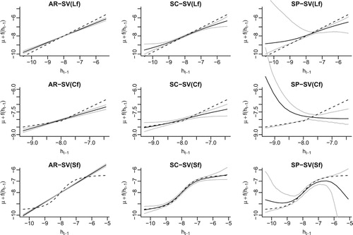
Figure 1. Estimated autoregressive function f for the unleveraged SV models based on a single simulated dataset. The dashed line in each graph shows the true functional form of f and the solid lines represent the posterior average of f as well as the 95% credible bands. For the semiparametric models SC-SV and SP-SV, the 20-knot-interval version is presented.

1. (Lf) Linear f: $h_t=-0.8+0.9h_{t-1}+{\xi }_t$. This is the basic SV model.

2. (Cf) Change-point f: $h_t=-8.1+0.9h_{t-1}^{\ast }I(h_{t-1}^{\ast }>0)+0.3h_{t-1}^{\ast }I(h_{t-1}^{\ast }\le 0)+{\xi }_t,$ where $h_{t-1}^{\ast }=h_{t-1}+8$. The slope of this autoregressive function is steeper when the lagged log volatility $h_{t-1}$ is greater than the change point, $-8$, which reflects the belief that the signal in the volatility process is stronger when the market is more volatile.

3. (Sf) Sigmoid f: $h_t=-8+1.6h_{t-1}^{\ast }/\sqrt{1+h_{t-1}^{\ast 2}}+{\xi }_t,$ where $h_{t-1}^{\ast }=h_{t-1}+8$. This particular sigmoid function produces a volatility series with a quasi-Markov-switching behaviour. The two states (volatile and stable) are generated by the two tails of the sigmoid function and the steepness of the curve in the middle controls the transition between the two states.

Table 1 summarises the estimated MSE and MAE of the posterior means of the log volatilities compared to their simulated values. When the autoregressive function is linear, i.e., when AR-SV is the correct model, the shape-constrained semiparametric model underperforms the AR-SV model by a small margin, while the SP-SV model, without proper shape constraints, is too flexible to pick up the linear form reliably. When the true autoregressive function is nonlinear, the impact of imposing the correct shape constraints on the estimation of the log volatilities becomes evident. For example, with the change-point autoregressive SV model, imposing shape constraints (i.e., the SC-SV model) reduces the MSE over the SP-SV model by 28% (10 knot intervals) and 30% (20 knot intervals) and the reduction in MSE for the sigmoid autoregressive SV model is 26% and 30% respectively. This evidences the gain from including shape constraints in a semiparametric SV model when they are warranted.

Table 1. For the three true unleveraged SV models (Lf , Cf and Sf ), a summary of the MSE and MAE of the log volatilities, $\{h_t{\}}_{t=1}^N$, obtained from fitting five different SV models. The averages and standard errors are multiplied by 100, and are based on 200 replicate series.

True Model		Fitted Models
		AR-SV	SC-SV(10)	SP-SV(10)	SC-SV(20)	SP-SV(20)
Lf
Average (s.e.)	MSE	36.3(0.2)	36.7(0.2)	40.2(0.4)	36.9(0.2)	43.2(0.6)
	MAE	47.9(0.1)	48.2(0.1)	50.4(0.3)	48.3(0.1)	52.2(0.3)
Rel. to AR-SV	MSE	100.0%	101.2%	110.7%	101.5%	119.0%
	MAE	100.0%	100.6%	105.1%	100.8%	108.9%
Cf		AR-SV	SC-SV(10)	SP-SV(10)	SC-SV(20)	SP-SV(20)
Average (s.e.)	MSE	24.7(0.1)	23.1(0.1)	31.9(0.3)	23.1(0.1)	33.2(0.3)
	MAE	39.4(0.1)	38.1(0.1)	44.7(0.2)	38.1(0.1)	46.0(0.2)
Rel. to AR-SV	MSE	100.0%	93.6%	129.3%	93.5%	134.7%
	MAE	100.0%	96.9%	113.6%	96.8%	116.8%
Sf		AR-SV	SC-SV(10)	SP-SV(10)	SC-SV(20)	SP-SV(20)
Average (s.e.)	MSE	38.2(0.2)	34.2(0.2)	46.5(0.6)	34.0(0.2)	48.5(0.7)
	MAE	49.1(0.1)	46.2(0.2)	55.7(0.4)	45.9(0.2)	57.1(0.4)
Rel. to AR-SV	MSE	100.0%	89.6%	121.8%	88.9%	126.9%
	MAE	100.0%	94.1%	113.5%	93.6%	116.3%

Our findings from Table 1 can be further confirmed by the fitted autoregressive functions shown in Figure 1. To simplify our presentation, we only display the 20-knot-interval version of the fitted semiparametric SV models (the 10-knot-interval version was less smooth, but exhibited similar patterns). The true autoregressive functions (denoted by the dark solid lines in each panel of the figure) are estimated by the posterior means of $f\left({\tilde{h}}_{t-1}\right)$ where ${\tilde{h}}_{t-1}$ is a grid of pre-specified values of $h_t$. It is clearly seen in Figure 1 that the estimated autoregressive functions for the semiparametric model without shape constraints (SP-SV) have very large posterior variance, especially toward the tails where the volatility data are scarce. Additionally, the posterior distribution of $f\left({\tilde{h}}_{t-1}\right)$ can be highly skewed and the posterior averages can deviate substantially from the truth (see the fitted f function for the change-point autoregressive model). Imposing proper shape constraints in the semiparametric model considerably reduces the posterior variance and skewness of the estimated autoregressive function across all values of the past volatilities, and the resulting SC-SV model is still flexible enough to capture the shapes of the different true autoregression functions.

4.2. Leveraged SV models

For the leveraged models, we consider the following three different volatility equations. (Plots of the true autoregressive and leverage functions are shown as the dashed lines in Figure 2.)

1. (Lf-Lg) Linear f & Linear g: $h_t=-0.9+0.9h_{t-1}-0.6{\epsilon }_{t-1}+{\xi }_t$ where ${\epsilon }_{t-1}=r_{t-1}\exp (-h_{t-1}/2)$. This is the AR-SV model with leverage effect.

2. (Lf-NLg) Linear f & Nonlinear g: $h_t=-1.1+0.9h_{t-1}-0.6{\epsilon }_{t-1}I({\epsilon }_{t-1}<0)+0.1{\epsilon }_{t-1}I({\epsilon }_{t-1}\ge 0)+{\xi }_t,$ where ${\epsilon }_{t-1}=r_{t-1}\exp (-h_{t-1}/2)$. If the variance of the error term ${\xi }_t$ is 0, this becomes the EGARCH model whose news impact curve is asymmetric and piecewise linear.

3. (NLf-NLg) Nonlinear f & Nonlinear g: $h_t=-8.5+0.9h_{t-1}^{\ast }I(h_{t-1}^{\ast }>0)+0.3h_{t-1}^{\ast }I(h_{t-1}^{\ast }\le 0)-0.6{\epsilon }_{t-1}I({\epsilon }_{t-1}<0)+0.1{\epsilon }_{t-1}I({\epsilon }_{t-1}\ge 0)+{\xi }_t,$ where $h_{t-1}^{\ast }=h_{t-1}+8$ and ${\epsilon }_{t-1}=r_{t-1}\exp (-h_{t-1}/2)$.

Figure 2. For the three true leveraged SV models (Lf-Lg, Lf-NLg and NLf-NLg), the estimated autoregressive function f (odd rows) and leverage function g (even rows) in different fitted models (columns). The legends are the same as in Figure 1.

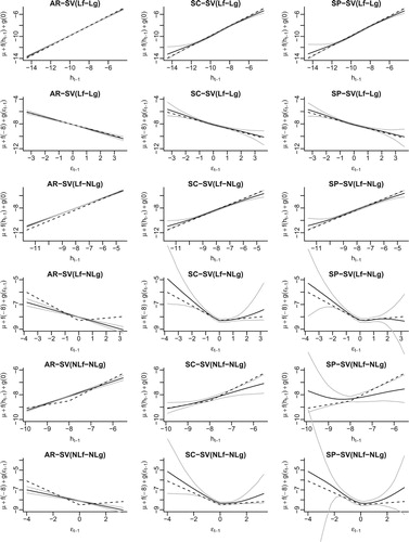
The variances of the ${\xi }_t$ terms in the above equations are set to be 0.15. We implement the correct shape constraints in the SC-SV models, which means that for the Lf-Lg case, the leverage function g is assumed to be monotonically decreasing on the entire real line while in the other two cases, it is assumed to be monotonically decreasing on the negative real line and monotonically increasing on the positive real line. The MSE and MAE of the estimated log volatilities compared to the simulated values are shown in Table 2.

Table 2. For the three true leveraged SV models (Lf-Lg, Lf-NLg and NLf-NLg), a summary of the MSE and MAE of the log volatilities, $\{h_t{\}}_{t=1}^N$, obtained from fitting five different SV models. The averages and standard errors are multiplied by 100, and are based on 200 replicate series.

True model		Fitted models
		AR-SV	SC-SV(10)	SP-SV(10)	SC-SV(20)	SP-SV(20)
Lf-Lg
Average (s.e.)	MSE	38.0(0.2)	39.5(0.2)	39.6(0.2)	39.7(0.2)	40.3(0.3)
	MAE	48.5(0.1)	49.6(0.1)	49.6(0.1)	49.7(0.1)	50.0(0.2)
Rel. to AR-SV	MSE	100.0%	104.2%	104.3%	104.7%	106.1%
	MAE	100.0%	102.3%	102.3%	102.5%	103.1%
Lf-NLg		AR-SV	SC-SV(10)	SP-SV(10)	SC-SV(20)	SP-SV(20)
Average (s.e.)	MSE	35.3(0.2)	30.9(0.1)	31.2(0.1)	31.0(0.1)	31.7(0.3)
	MAE	47.2(0.1)	44.3(0.1)	44.6(0.1)	44.4(0.1)	44.8(0.1)
Rel. to AR-SV	MSE	100.0%	87.5%	88.5%	87.9%	89.6%
	MAE	100.0%	93.9%	94.4%	94.2%	94.9%
NLf-NLg		AR-SV	SC-SV(10)	SP-SV(10)	SC-SV(20)	SP-SV(20)
Average (s.e.)	MSE	25.5(0.1)	21.8(0.1)	26.3(0.3)	22.0(0.1)	27.0(0.3)
	MAE	40.2(0.1)	37.4(0.1)	41.2(0.3)	37.6(0.1)	41.9(0.3)
Rel. to AR-SV	MSE	100.0%	85.5%	103.2%	86.4%	105.9%
	MAE	100.0%	93.0%	102.4%	93.6%	104.2%

When the autoregressive component f and the leverage function g are both linear, AR-SV is the true model and as expected, it outperforms both semiparametric models. When either f or g is nonlinear, however, the AR-SV model is not flexible enough to pick up the true functional forms, resulting in the larger MSE and MAE as compared to the shape-constrained semiparametric model. For all three forms of the volatility function, the advantage of incorporating shape constraints in the semiparametric models is reflected in the consistently smaller MSE and MAE for the SC-SV model over the SP-SV model. As in Section 4.1, the greatest gain in the MSE and MAE was obtained when the autoregressive function f deviates the most from linearity (the NLf-NLg case).

Figure 2 shows the estimated autoregressive function f (odd rows) and leverage function g (even rows). Whenever the true autoregressive or leverage function is nonlinear, the fitted f or g functions in the semiparametric SV model without shape constraints (SP-SV) can have extremely large posterior variance toward the tails where the data are scarce. Restricting the parameter space through proper shape constraints proves to be essential for more efficient estimation in SV models.

5. Empirical studies

We now assess the advantage of our proposed shape-constrained semiparametric additive SV models for the prediction of volatilities in four real-world equity returns: the S&P500 index, Equity Residential (EQR; a real estate investment trust), Microsoft (MSFT), and Johnson & Johnson (JnJ). The returns are calculated as the change in the logarithm of the daily adjusted closing prices obtained from Yahoo! Finance. For each series, we use the returns from November 1, 2001 to October 29th, 2010 as our training set and the following three years of returns from November 1, 2010 to October 31, 2013 as the test set. For both the training and test return series, we subtract the sample mean from the data so that the returns have zero mean.

As in our simulation studies, we consider the parametric model (AR-SV), the semiparametric additive SV model with shape constraints (SC-SV) and without shape constraints (SP-SV). We fit both a leveraged and an unleveraged version of each model and compare their predictive log likelihoods over the test period. We run the MCMC for 1,02,500 iterations with the first 2500 draws discarded as burn-in samples and the remaining draws thinned every 25 iterations. In terms of the shape constraints in the SC-SV model, exploratory analyses indicated that it is reasonable to assume the autoregressive function f to be monotonically increasing and the leverage function g monotonically decreasing. These assumptions will be assessed later. We use K=20 basis functions for f and L=20 basis functions for g. The predictive log likelihood that we use to compare the models is calculated according to Section 3.2 with the step size $S_0$ for the multiple-step prediction set to be 110.

Table 3 displays the estimated predictive log likelihoods for all six SV models. For each of the four return series, the value in bold denotes the model with the largest predictive log likelihood. The predictive log likelihood of the semiparametric model without shape constraints always lags behind the corresponding shape-constrained model, suggesting that it is desirable to incorporate shape constraints in our semiparametric additive model when the knowledge of the true functional shapes is available. Compared to the AR-SV model, the semiparametric model without shape constraints only outperforms the corresponding AR-SV model in three out of the eight pairs. However, imposing shape constraints increases this ratio to seven out of eight. For Equity Residential, the outperformance of the shape-constrained model compared to AR-SV is substantial. In one case, Johnson & Johnson, the linear parametric AR-SV model seems to be the most suitable model, indicating that a more parsimonious model is preferred for explaining the volatility in this return series.

Table 3. Predictive log likelihood of daily returns from November 1, 2010 to October 31, 2013 using six different SV models. (u) – unleveraged; (l) – leveraged. The results of the best performing model (those with the largest predictive log likelihood) are in bold face.

	AR-SV(u)	SC-SV (u)	SP-SV (u)	AR-SV(l)	SC-SV (l)	SP-SV (l)
S&P500	−3798.8	−3796.5	−3799.3	−3784.5	−3784.2	−3786.0
EQR	−4080.5	−4068.8	−4072.0	−4080.4	−4070.6	−4079.5
MSFT	−4103.6	−4100.7	−4100.8	−4102.6	−4099.4	−4103.1
JnJ	−3681.7	−3682.9	−3684.2	−3680.9	−3680.7	−3681.7

To assess the appropriateness of our shape assumptions for the four equity returns, we estimate the autoregressive function f and leverage function g in the same way as in the simulation studies. Figure 3 shows the fitted functions (posterior mean) and the associated pointwise 95% credible bands for the leveraged semiparametric SV models (with and without the shape constraints) for each return series.

Figure 3. Fitted autoregressive function f and leverage function g for the daily returns of the S&P500, EQR, MSFT and JnJ. The solid lines show the posterior means and 95% credible bands of the fitted functions in the leveraged semiparametric models with shape constraints while the dashed lines represent the posterior means and 95% credible bands in the leveraged semiparametric models without shape constraints.

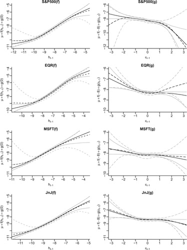
For the S&500 index, both fitted functions are clearly nonlinear, which means that the volatility process and consequently the return series are nonstationary. When the lagged log volatility $h_{t-1}$ is small, the lag one autocorrelation for fixed ${\epsilon }_{t-1}$ is diminished as compared to when $h_{t-1}$ is moderate; when $h_{t-1}$ is large, the lag one autocorrelation is also attenuated, but to a lesser degree. In addition, the shapes of the autoregressive and leverage functions estimated from the two semiparametric models (SC-SV and SP-SV) agree with each other for the most part: the function f is monotonically increasing and g monotonically decreasing. This means that our assumptions of the shape constraints are appropriate. Even though the leftmost section of the g function is found to be increasing in the SP-SV model, we find this counterintuitive and also unreliable since our simulation studies showed that the estimated functions towards the boundaries can deviate considerably from the truth if no shape constraints are implemented.

As for the other three return series, it can be seen that our monotonicity assumptions for the autoregressive and leverage functions in the shape-constrained models hold for all except the Equity Residential series (EQR). For EQR, the SP-SV model finds that the posterior mean of the leverage function g is increasing on the positive real line but with a very large degree of uncertainty. As a further investigation, we fit two additional shape-constrained models with the same priors on f and on $g\left({\epsilon }_{t-1}\right)$ for ${\epsilon }_{t-1}<0$. In the first model, we assumed the leverage function g to be monotonically increasing on the positive real line, but we imposed no shape constraints on $g\left({\epsilon }_{t-1}\right)$ for ${\epsilon }_{t-1}>0$ in the second one. Their predictive log likelihoods are $-4074.3$ and $-4074.5$ respectively, both larger than the predictive log likelihoods for the corresponding leveraged AR-SV and SP-SV models. However, neither of these two additional models outperforms the original leveraged SC-SV model with the monotonicity constraint on g. This may be due to the fact that the lagged return innovation ${\epsilon }_{t-1}$ follows the standard normal distribution a priori, which means that it would be rare to observe an extreme ${\epsilon }_{t-1}$ out in the tails. Nevertheless, a monotonically decreasing leverage function seems a reasonable assumption for fitting the shape-constrained semiparametric additive SV models on most equity returns.

6. Conclusion

In this article, we have proposed a class of shape-constrained semiparametric additive stochastic volatility models. We have introduced a parameterisation that allows for more efficient sampling from the posterior distribution, and developed a particle-filter-based model comparison approach. Through simulations and empirical studies, we demonstrated that the shape-constrained semiparametric SV model has the flexibility to capture unknown functional shapes, while not losing too much efficiency compared to a parametric SV model when the true underlying model is best explained by the latter.

We demonstrated the use of specific forms of shape constraints on the autoregressive and leverage function, but we note that within this framework, researchers and practitioners can easily incorporate other shape constraints that they deem appropriate. Furthermore, our methodology of modelling the shape constraints in SV models can also be applied to other nonlinear state space models, such as the stochastic conditional duration (SCD) model (Bauwens & Veredas, 2004), to efficiently capture nonlinear features of the state equation. In this article we have fixed the number of basis functions for the nonlinear functions f and g (as denoted by K and L respectively) to be 10 or 20 – more generally we can use the Bayes Factor to select between different numbers of basis functions.

Our shape-constrained SV model can be extended in a number of directions, beyond simply including additional lagged terms. First, the additivity between the autoregressive and leverage function can be relaxed. One option would be to assume that the log volatility satisfies $h_t=\zeta (h_{t-1},{\epsilon }_{t-1})+{\xi }_t$ where the function ζ is subject to a two-dimensional shape constraint. The challenge lies in the fact that this function ζ does not have a rectangular support because of the dependence between $h_{t-1}$ and ${\epsilon }_{t-1}$. Alternatively, we can assume that the additivity holds on a different scale, $\varsigma \left({\sigma }_t\right)$, where ς can be a known function other than $\exp \left(h_t/2\right)$ – the $\exp \left(h_t/{\lambda }_0\right)$ scale considered by Comte (2004) would be an example. Second, the idea of incorporating shape constraints in semiparametric SV models can also be applied to additive GARCH-type models for more efficient estimation of the news impact curve. Third, our framework can be adapted to include convexity constraints on the functional components. Under the basis expansion (4(4) $q\left(x\right)={\beta }_0+{\beta }_1{w}_1\left(x\right)+\cdots +{\beta }_J{w}_J\left(x\right).$(4) ) and with the same basis functions (5(5) $\begin{array}{r}{w}_j\left(x\right)=\left\{\begin{array}{l}I(x>{\gamma }_{j-1})[min(x,{\gamma }_j)-{\gamma }_{j-1}]-({\gamma }_j-{\gamma }_{j-1})\\ \text{if }1\le j<M;\\ I(x>{\gamma }_{j-1})[min(x,{\gamma }_j)-{\gamma }_{j-1}]\\ \text{if }M\le j\le J,\end{array}\right.\end{array}$(5) ), convexity constraints can be translated to the ordering of the slope coefficients $\{{\beta }_k{\}}_{k=1}^K$. To constrain the function to be convex and monotonically increasing at the same time, the slope coefficients need to satisfy $0\le {\beta }_1\le {\beta }_2\le \cdots \le {\beta }_K$ and the model fitting is straightforward.

There are also several ways to improve our MCMC algorithm, especially the updating of the high-dimensional state vector. First, since the state variables are highly correlated with each other, updating more than one state variable at a time, i.e., using block updating (e.g., Chib & Greenberg, 1994, 1995), would be more efficient than the one-at-a-time updating. Second, we can improve the proposal distributions for updating the state variables by exploiting the shape of the full-conditional distribution, such as using the Metropolis-adjusted Langevin algorithm (Grenander & Miller, 1994; Roberts & Tweedie, 1996) and its variations. Finally, particle-filter-based methods, such as the Particle Markov chain Monte Carlo (PMCMC) method (e.g., Andrieu, Doucet, & Holenstein, 2010), can be applied as well.

Disclosure statement

No potential conflict of interest was reported by the authors.

Additional information

Funding

Peter Craigmile and Jiangyong Yin were supported in part by the National Science Foundation (NSF) under grant DMS-0906864. Xinyi Xu, Jiangyong Yin and Steven MacEachern were supported in part by the NSF under grant DMS-1209194. Peter Craigmile is additionally supported in part by the NSF under grants SES-1024709, DMS-1407604 and SES-1424481, and the National Cancer Institute of the National Institutes of Health under Award Number 1R21CA212308-01, and the project title is ‘Evaluating how licensing-law strategies will change neighborhood disparities in tobacco retailer density’. Xinyi Xu and Steven MacEachern are supported under grant DMS-1613110.

Notes on contributors

Jiangyong Yin

Jiangyong Yin was a Ph.D. student at The Ohio State University, and is currently working at CapitalG, San Francisco, California.

Peter F. Craigmile

Peter F. Craigmile is Professor at Department of Statistics, The Ohio State University.

Xinyi Xu

Xinyi Xu is an Associate Professor at Department of Statistics, The Ohio State University.

Steven MacEachern

Steven MacEachern is Professor at Department of Statistics, The Ohio State University.

Appendix

 

Updating ${\beta }_k$ and ${\beta }_k^{\ast }$ in the semiparametric SV model (6): Without sign constraints on ${\beta }_k$ (i.e., no shape constraints on the autoregressive function f), we draw ${\beta }_k={\beta }_k^{\ast }$ from its normal full conditional distribution whose mean and variance are given as $\begin{array}{rl}{\tilde{\mu }}_k& =\frac{{\tau }_k^{2^{\ast }}}{{\sigma }_k^{2^w}+{\tau }_k^{2^{\ast }}}{\mu }_k^w+\frac{{\sigma }_k^{2^w}}{{\sigma }_k^{2^w}+{\tau }_k^{2^{\ast }}}{\mu }_k^{\ast }\text{and}\\ & {\tilde{\tau }}_k^2=\frac{{\sigma }_k^{2^w}{\tau }_k^{2^{\ast }}}{{\sigma }_k^{2^w}+{\tau }_k^{2^{\ast }}}.\end{array}$ In the above equations, ${\mu }_k^{\ast }$ and ${\tau }_k^{2^{\ast }}$ are the conditional prior mean and variance of ${\beta }_k^{\ast }$, whereas ${\mu }_k^w$ and ${\tau }_k^{2^w}$ reflect the new information about ${\beta }_k^{\ast }$ in the data. If we use a flat prior for the initial state of the random walk prior of $\{{\beta }_k^{\ast }{\}}_{k=1}^K$, we have $\begin{array}{rl}{\mu }_k^{\ast }& =\left\{\begin{array}{ll}{\beta }_{k+1}^{\ast }& \text{if }k=1\\ {\beta }_{k-1}^{\ast }& \text{if }k=K\\ ({\beta }_{k-1}^{\ast }+{\beta }_{k+1}^{\ast })/2& \text{otherwise};\end{array}\right.\text{and}\\ {\tau }_k^{2^{\ast }}& =\left\{\begin{array}{ll}{\tau }^2& \text{if }k=1\text{ or }K\\ {\tau }^2/2& \text{otherwise}.\end{array}\right.\end{array}$ From the likelihood, we can obtain that ${\mu }_k^w=\sum _{t=2}^T{w}_k\left(h_{t-1}\right)e_k\left(t\right)/\sum _{t=2}^T{w}_k^2\left(h_{t-1}\right)$ and ${\sigma }_k^{2^w}={\sigma }^2/\sum _{t=2}^T{w}_k^2\left(h_{t-1}\right),$ where $e_k\left(t\right)=h_t-\mu -\sum _{l=1}^L{v}_l\left({\epsilon }_{t-1}\right){\alpha }_l-\sum _{j=1,j\ne k}^K{w}_j\left(h_{t-1}\right){\beta }_j$. We can see that for ${\mu }_k^w$ and ${\sigma }_k^{2^w}$ to exist, the corresponding basis function evaluated at $h_{t-1}$, $w_k\left(h_{t-1}\right)$, needs to be non-zero for at least some $t\ge 2$. However, this is not always guaranteed since by the definition of the basis functions (5(5) $\begin{array}{r}{w}_j\left(x\right)=\left\{\begin{array}{l}I(x>{\gamma }_{j-1})[min(x,{\gamma }_j)-{\gamma }_{j-1}]-({\gamma }_j-{\gamma }_{j-1})\\ \text{if }1\le j<M;\\ I(x>{\gamma }_{j-1})[min(x,{\gamma }_j)-{\gamma }_{j-1}]\\ \text{if }M\le j\le J,\end{array}\right.\end{array}$(5) ), when $k\ge M$, $w_k\left(h_{t-1}\right)=0$ for $h_{t-1}<{\gamma }_{k-1}$ and when k<M, $w_k\left(h_{t-1}\right)=0$ for $h_{t-1}>{\gamma }_k$. In other words, $w_k\left(h_{t-1}\right)$ would be zero for all $t\ge 2$ if all values of $\{h_{t-1}{\}}_{t=2}^T$ simulated in one MCMC iteration are below ${\gamma }_{k-1}$ for $k\ge M$ or above ${\gamma }_k$ for k<M. When this happens, we draw ${\beta }_k^{\ast }$ from its conditional prior distribution $N({\mu }_k^{\ast },{\tau }_k^{2^{\ast }})$.

If ${\beta }_k$ is constrained to be positive a priori, i.e., ${\beta }_k=I({\beta }_k^{\ast }>0){\beta }_k^{\ast }$, Neelon and Dunson (2004) shows that the full conditional of ${\beta }_k^{\ast }$ can be expressed as a mixture of two truncated normal distributions. Let $\mathrm{\Phi }(\cdot ;m,v)$ be the cumulative distribution function of a N(m, v) random variable, $\phi (\cdot ;m,v)$ be the corresponding density function and tN$({\mu }_0,{\sigma }_0^2$; $[a,b])$ denote the truncated Normal distribution with support $[a,b]$. Then a MCMC draw for ${\beta }_k^{\ast }$ is simply a draw from a tN$({\mu }_k^{\ast }$, ${\tau }_k^{2^{\ast }}$; $(-\mathrm{\infty },0])$ distribution with probability proportional to $\mathrm{\Phi }(0;{\mu }_k^{\ast },{\tau }_k^{2^{\ast }})/\phi (0;{\mu }_k^{\ast },{\tau }_k^{2^{\ast }})$ and from a tN$({\tilde{\mu }}_k$, ${\tilde{\tau }}_k^2$; $[0,\mathrm{\infty }))$ distribution with probability proportional to $[1-\mathrm{\Phi }(0;{\tilde{\mu }}_k,{\tilde{\tau }}_k^2\left)\right]/\phi (0;{\tilde{\mu }}_k,{\tilde{\tau }}_k^2)$.

 

Updating ${\alpha }_l$ and ${\alpha }_l^{\ast }$ in the semiparametric SV model (6): The difference between updating ${\alpha }_l$ and ${\beta }_k$ lies in the fact that both positive and negative sign constraints for ${\alpha }_l$ are considered in (8(8) $\begin{array}{rl}{\alpha }_1^{\ast }& \sim \pi \left({\alpha }_1^{\ast }\right);\\ {\alpha }_l^{\ast }& \sim N({\alpha }_{l-1}^{\ast },{\gamma }^2),l\ge 2;\\ {\alpha }_l& =I({\alpha }_l^{\ast }<0){\alpha }_l^{\ast },l\le M-1;\end{array}$(8) ) and (9(9) $\begin{array}{rl}{\alpha }_l& =\iota \left({\alpha }_l^{\ast }\right){\alpha }_l^{\ast },l\ge M.\end{array}$(9) ). Without sign constraints on ${\alpha }_l$ (i.e., without shape constraints on the leverage function g), the full conditional distribution of ${\alpha }_l^{\ast }$ is similar to that of ${\beta }_k^{\ast }$. When ${\alpha }_l$ is constrained to be positive, the full conditional distribution of ${\alpha }_l^{\ast }$ is again similar to that of ${\beta }_k^{\ast }$ for positive ${\beta }_k$. However, when ${\alpha }_l$ is constrained to be negative, the full conditional distribution of ${\alpha }_l^{\ast }$ is a mixture of two truncated normal distributions whose positive part now depends on the conditional prior mean and variance and the negative part on the data.

References

- Andrieu, C., Doucet, A., & Holenstein, R. (2010). Particle Markov chain Monte Carlo methods. Journal of the Royal Statistical Society: Series B (Statistical Methodology), 72, 269–342. doi: 10.1111/j.1467-9868.2009.00736.x
- Bauwens, L., & Veredas, D. (2004). The stochastic conditional duration model: A latent variable model for the analysis of financial durations. Journal of Econometrics, 119, 381–412. doi: 10.1016/S0304-4076(03)00201-X
- Brezger, A., & Steiner, W. J. (2008). Monotonic regression based on Bayesian P–splines. Journal of Business & Economic Statistics, 26, 90–104. doi: 10.1198/073500107000000223
- Cai, B., & Dunson, D. (2007). Bayesian multivariate isotonic regression splines. Journal of the American Statistical Association, 102, 1158–1171. doi: 10.1198/016214506000000942
- Chib, S., & Greenberg, E. (1994). Bayes inference in regression models with ARMA(p,q) errors. Journal of Econometrics, 64, 183–206. doi: 10.1016/0304-4076(94)90063-9
- Chib, S., & Greenberg, E. (1995). Understanding the Metropolis-Hastings algorithm. The American Statistician, 49, 327–335.
- Comte, F. (2004). Kernel deconvolution of stochastic volatility models. Journal of Time Series Analysis, 25, 563–582. doi: 10.1111/j.1467-9892.2004.01825.x
- Eddelbuettel, D., & Sanderson, C. (2014). RcppArmadillo: Accelerating R with high-performance C++ linear algebra. Computational Statistics & Data Analysis, 71, 1054–1063. doi: 10.1016/j.csda.2013.02.005
- Engle, R. (1982). Autoregressive conditional heteroscedasticity with estimates of the variance of United Kingdom inflation. Econometrica, 50, 987–1007. doi: 10.2307/1912773
- Engle, R., & Gonzalez-Rivera, G. (1991). Semiparametric ARCH models. Journal of Business & Economic Statistics, 9, 345–359.
- Engle, R., & Ng, V. (1993). Measuring and testing the impact of news on volatility. The Journal of Finance, 48, 1749–1778. doi: 10.1111/j.1540-6261.1993.tb05127.x
- Godsill, S. J., Doucet, A., & West, M. (2004). Monte Carlo smoothing for nonlinear time series. Journal of the American Statistical Association, 99, 156–168. doi: 10.1198/016214504000000151
- Gordon, N. J., Salmond, D. J., & Smith, A. F. (1993). Novel approach to nonlinear/non-Gaussian Bayesian state estimation. IEEE Proceedings F (Radar and Signal Processing), 140, 107–113. doi: 10.1049/ip-f-2.1993.0015
- Grenander, U., & Miller, M. I. (1994). Representations of knowledge in complex systems. Journal of the Royal Statistical Society. Series B (Methodological), 56, 549–603. doi: 10.1111/j.2517-6161.1994.tb02000.x
- Harvey, A. C., & Shephard, N. (1996). Estimation of an asymmetric stochastic volatility model for asset returns. Journal of Business & Economic Statistics, 14, 429–434.
- Hull, J., & White, A. (1987). The pricing of options on assets with stochastic volatilities. The Journal of Finance, 42, 281–300. doi: 10.1111/j.1540-6261.1987.tb02568.x
- Kim, S., Shephard, N., & Chib, S. (1998). Stochastic volatility: Likelihood inference and comparison with ARCH models. The Review of Economic Studies, 65, 361–393. doi: 10.1111/1467-937X.00050
- Liu, J. S., & Chen, R. (1998). Sequential Monte Carlo methods for dynamic systems. Journal of the American Statistical Association, 93, 1032–1044. doi: 10.1080/01621459.1998.10473765
- Meyer, M. C., Hackstadt, A. J., & Hoeting, J. A. (2011). Bayesian estimation and inference for generalised partial linear models using shape-restricted splines. Journal of Nonparametric Statistics, 23, 867–884. doi: 10.1080/10485252.2011.597852
- Nakajima, J., & Omori, Y. (2009). Leverage, heavy-tails and correlated jumps in stochastic volatility models. Computational Statistics & Data Analysis, 53, 2335–2353. doi: 10.1016/j.csda.2008.03.015
- Neelon, B., & Dunson, D. (2004). Bayesian isotonic regression and trend analysis. Biometrics, 60, 398–406. doi: 10.1111/j.0006-341X.2004.00184.x
- Nelson, D. (1991). Conditional heteroskedasticity in asset returns: A new approach. Econometrica, 59, 347–370. doi: 10.2307/2938260
- Omori, Y., Chib, S., Shephard, N., & Nakajima, J. (2007). Stochastic volatility with leverage: Fast and efficient likelihood inference. Journal of Econometrics, 140, 425–449. doi: 10.1016/j.jeconom.2006.07.008
- R Core Team (2013). R: A Language and Environment for Statistical Computing. R Foundation for Statistical Computing, Vienna, Austria. URL http://www.R-project.org/.
- Ramsay, J. (1988). Monotone regression splines in action. Statistical Science, 3, 425–441. doi: 10.1214/ss/1177012761
- Roberts, G. O., & Tweedie, R. L. (1996). Exponential convergence of Langevin distributions and their discrete approximations. Bernoulli, 2, 341–363. doi: 10.2307/3318418
- Rydberg, T. (2000). Realistic statistical modelling of financial data. International Statistical Review, 68, 233–258. doi: 10.1111/j.1751-5823.2000.tb00329.x
- Taylor, S. (1994). Modeling stochastic volatility: A review and comparative study. Mathematical Finance, 4, 183–204. doi: 10.1111/j.1467-9965.1994.tb00057.x
- Yu, J. (2005). On leverage in a stochastic volatility model. Journal of Econometrics, 127, 165–178. doi: 10.1016/j.jeconom.2004.08.002
- Yu, J. (2012). A semiparametric stochastic volatility model. Journal of Econometrics, 167, 473–482. doi: 10.1016/j.jeconom.2011.09.029
Appendix
Updating and
in the semiparametric SV model (6): Without sign constraints on
(i.e., no shape constraints on the autoregressive function f), we draw
from its normal full conditional distribution whose mean and variance are given as
In the above equations,
and
are the conditional prior mean and variance of
, whereas
reflect the new information about
in the data. If we use a flat prior for the initial state of the random walk prior of
, we have
From the likelihood, we can obtain that
where
. We can see that for
to exist, the corresponding basis function evaluated at
,
, needs to be non-zero for at least some
. However, this is not always guaranteed since by the definition of the basis functions (Equation5
(5)
(5) ), when
for
and when k<M,
. In other words,
would be zero for all
if all values of
simulated in one MCMC iteration are below
or above
for k<M. When this happens, we draw
from its conditional prior distribution
.
If is constrained to be positive a priori, i.e.,
, Neelon and Dunson (Citation2004) shows that the full conditional of
can be expressed as a mixture of two truncated normal distributions. Let
be the cumulative distribution function of a N(m, v) random variable,
be the corresponding density function and tN
;
denote the truncated Normal distribution with support
. Then a MCMC draw for
is simply a draw from a tN
distribution with probability proportional to
and from a tN
in the semiparametric SV model (6): The difference between updating
lies in the fact that both positive and negative sign constraints for
are considered in (Equation8
(8)
(8) ) and (Equation9
(9)
(9) ). Without sign constraints on
(i.e., without shape constraints on the leverage function g), the full conditional distribution of
is similar to that of
. When
is constrained to be positive, the full conditional distribution of
is again similar to that of
for positive
. However, when
is constrained to be negative, the full conditional distribution of
is a mixture of two truncated normal distributions whose positive part now depends on the conditional prior mean and variance and the negative part on the data.