A discussion of ‘prior-based Bayesian information criterion (PBIC)’

Professors Bayarri, Berger, Jang, Ray, Pericchi, and Visser deserve a special congratulation for their great work on Bayesian model and variable selection and a pioneering idea of prior-based Bayesian information criterion (PBIC). This work opens the door for contemporary advances in the difficult problem of model and variable selection.

There exist three types of commonly used Bayesian approaches. The first type works on information criterion, such as the well-known BIC. The newly proposed PBIC belongs to this category. The second type includes the indicator model selection (see, e.g., Brown, Vannucci, & Fearn, 1998; Dellaportas, Forster, & Ntzoufras, 1997; George & McCulloch, 1993; Kuo & Mallick, 1998; Yuan & Lin, 2005), the stochastic search method (e.g., O'Hara & Sillanpää, 2009), and the model space method by Green (1995). The third type, which is considered in this discussion, is to apply priors on the regression coefficients that promotes the shrinkage of coefficients towards 0. This last type of approaches is intrinsically connected with frequentist methods in the sense that, first of all, such priors play the same role as the assumption that the coefficients are sparse for the frequentist approach and secondly, in some sense, the Bayesian solution is equivalent to the corresponding frequentist counterpart with a certain penalty parameter. Typical research papers for this type include Griffin and Brown (2009), Park and Casella (2008), and Kyung, Gilly, Ghosh, and Casella (2010).

The shrinkage prior approach may not provide sparse estimates of regression coefficients in general, which could not only complicate the interpretation but also inflate statistical error in analysis. Even without a well-defined variable selection approach, a Bayesian analysis based on a subset of covariates with size considerably less than the original dimensionality, which is referred to as sparse Bayesian analysis, could produce better results than the Bayesian analysis based on all covariates. Several attempts have been made to obtain sparse Bayesian estimates based on shrinkage priors. For instance, Hoti and Sillanpää (2006) proposed a method based on thresholding; however, the method is based on certain approximations, and the choice of the threshold is ad hoc. Another example is the sparse Bayesian learning by Tipping (2001), but it involves complicated nonconvex optimisation and assumes that the variance of the error term is known.

Under the framework of shrinkage priors, we consider a Bayesian variable selection method via a benchmark variable. The benchmark variable serves as a standard to measure the importance of each variable based on the posterior distribution of the corresponding coefficient.

As the first attempt, we focus on linear regression models with normally distributed errors. Let $\mathit{y}$ be an n-dimensional vector of response and, without loss of generality, let ${\mathit{x}}_1,\dots ,{\mathit{x}}_p$ be p centralised n-dimensional vectors of predictors or covariates. Conditional on $\mathit{X}=({\mathit{x}}_1,\dots ,{\mathit{x}}_p)$, $\mathit{y}$ is assumed to be multivariate normally distributed as $N({\beta }_0\mathbf{\text{1}}+\mathit{X}\mathit{\beta },{\sigma }^2\mathit{I})$, where $\mathit{\beta }$ is a p-dimensional column vector whose jth component is ${\beta }_j$, ${\beta }_0,{\beta }_1,\dots ,{\beta }_p$ are p+1 unknown parameters, σ is an unknown positive parameter, $\mathbf{\text{1}}$ is a $n-$dimensional vector with all components 1 and $\mathit{I}$ is the identity matrix of order n.

Consider the following prior density on $\mathit{\beta }$ conditioned on ${\sigma }^2$, (1) $p\left(\mathit{\beta }|{\sigma }^2\right)=\prod _{i=1}^p\frac{{\lambda }^{1/\delta }}{2^{1/\delta }\mathrm{\Gamma }\left(1/\delta \right)\sigma }\exp \left(-2\lambda {\left|\frac{{\beta }_i}{2\sigma }\right|}^{\delta }\right)$(1) where $\lambda >0$ and $1\le \delta \le 2$ are hyper-parameters. When $\delta =1$, this is the Laplace prior which was considered by Park and Casella (2008) for their Bayesian Lasso. When $\delta =2$, the prior in (1(1) $p\left(\mathit{\beta }|{\sigma }^2\right)=\prod _{i=1}^p\frac{{\lambda }^{1/\delta }}{2^{1/\delta }\mathrm{\Gamma }\left(1/\delta \right)\sigma }\exp \left(-2\lambda {\left|\frac{{\beta }_i}{2\sigma }\right|}^{\delta }\right)$(1) ) is a multivariate normal density and produces the posterior mode of $\mathit{\beta }$ equivalent to the ridge regression estimate. As the Laplace prior is ‘sharper’ than the Gaussian one, it is expected to yield more sparse predictive models with the potentiality of easier interpretation, which is especially desirable for high-dimensional data with a considerably large amount of noisy variables. However, the posterior inferences associated with Laplace prior involves relatively intensive computation.

For ${\beta }_0$ and ${\sigma }^2$ that are not involved with variable selection, we consider noninformative priors so that the overall prior for all parameters is $p({\beta }_0,\mathit{\beta },{\sigma }^2)\propto \frac{1}{{\sigma }^2}p\left(\mathit{\beta }|{\sigma }^2\right)$ If the posterior distribution of ${\beta }_i$ is nearly the same as that from a noise variable centred at 0, then it is natural to eliminate ${\mathit{x}}_i$ as an unimportant covariate. However, the question is how to quantify whether a posterior distribution to be close to that of a noise.

To illustrate our idea, let us first consider an artificial case where a covariate $\mathit{z}$ exists and is known to have no effect on $\mathit{y}$. For example, $\mathit{y}$ is distributed as $N(\mathit{z}{\beta }_z+\mathbf{1}{\beta }_0+\mathit{X}\mathit{\beta },{\sigma }^2\mathit{I})$ with ${\beta }_z=0$. Although we know $\mathit{z}$ is redundant, we still put a prior on ${\beta }_z$ such that ${\beta }_z$ and ${\beta }_i$ are independently identically distributed conditioning on ${\sigma }^2$. Under this setting, ${\mathit{x}}_i$ could be treated as an unimportant variable if the posterior of ${\beta }_i$ is similar to the posterior of ${\beta }_z$. In other words, the variable $\mathit{z}$ serves as a benchmark in measuring the importance of ${\mathit{x}}_i$'s.

A benchmark variable should have a posterior distribution centred at 0 and should not affect the Bayesian analysis concerning $\mathit{\beta }$. The question is, how do we find a benchmark variable when we do not have a redundant variable at hand?

We now show that there is a universal solution. Since $\mathit{X}$ is column-wisely centralised, the density of $\mathit{y}$ given $(\mathit{X},\mathit{z},{\beta }_0,\mathit{\beta },{\beta }_z,{\sigma }^2)$ is $\begin{array}{rl}& p(\mathit{y}|\mathit{X},\mathit{z},{\beta }_0,\mathit{\beta },{\beta }_z,{\sigma }^2)\\ & \propto \frac{1}{{\sigma }^n}\exp \left(-\frac{{\left|\left|\mathit{y}-\mathit{z}{\beta }_z-\mathbf{1}{\beta }_0-\mathit{X}\mathit{\beta }\right|\right|}^2}{2{\sigma }^2}\right)\\ & =\frac{1}{{\sigma }^n}\exp \\ & \times \left(-\frac{\begin{array}{c}{\left|\left|\tilde{\mathit{y}}-\mathit{X}\mathit{\beta }\right|\right|}^2+{\left|\left|\mathit{z}-\overline{z}\mathbf{\text{1}}\right|\right|}^2{\beta }_z^2-2{\beta }_z{\mathit{z}}^{\prime }\\ (\tilde{\mathit{y}}-\mathit{X}\mathit{\beta })+n({\beta }_0-\overline{y}+{\beta }_z\overline{\mathit{z}}{)}^2\end{array}}{2{\sigma }^2}\right)\end{array}$ where $\overline{y}$ is the average of components of $\mathit{y}$, $\overline{z}$ is the average of components of $\mathit{z}$, $\tilde{\mathit{y}}=\mathit{y}-\overline{y}\mathbf{\text{1}}$, ${\left|\left|\mathit{a}\right|\right|}^2={\mathit{a}}^{\prime }\mathit{a}$, and ${\mathit{a}}^{\prime }$ is the transpose of $\mathit{a}$. Under the previously described prior, the joint conditional posterior distribution $p({\beta }_0,\mathit{\beta },{\beta }_z|\mathit{X},\mathit{z},\mathit{y},{\sigma }^2)$ can be obtained. Since the intercept ${\beta }_0$ is not of interest, we integrate it out from $p({\beta }_0,\mathit{\beta },{\beta }_z|\mathit{X},\mathit{z},\mathit{y},{\sigma }^2)$ and obtain the conditional posterior density of $(\mathit{\beta },{\beta }_z)$ given $(\mathit{X},\mathit{z},\mathit{y},{\sigma }^2)$ as follows: (2) $\begin{array}{rl}& p\left(\mathit{\beta },{\beta }_z|\mathit{X},\mathit{z},\mathit{y},{\sigma }^2\right)\\ & \propto \frac{1}{{\sigma }^{n+1}}\\ & \times \left[p\left(\mathit{\beta }|{\sigma }^2\right)\exp \left(-\frac{{\left|\left|\tilde{\mathit{y}}-\mathit{X}\mathit{\beta }\right|\right|}^2+2{\beta }_z{\mathit{z}}^{\prime }\mathit{X}\mathit{\beta }}{2{\sigma }^2}\right)\right]\\ & \times \left[p\left({\beta }_z|{\sigma }^2\right)\exp \left(-\frac{{\left|\left|\mathit{z}-\overline{z}\mathbf{\text{1}}\right|\right|}^2{\beta }_z^2-2{\mathit{z}}^{\prime }\tilde{\mathit{y}}{\beta }_z}{2{\sigma }^2}\right)\right]\end{array}$(2) Note that marginalisation over ${\beta }_0$ is equivalent to centralising the response $\mathit{y}$. After the integration, it could be regarded that the posterior inferences are drawn from the centralised response $\tilde{\mathit{y}}$ instead of the original $\mathit{y}$. The reason that we introduce ${\beta }_0$ in the model and then integrate it out, instead of eliminating it at the very beginning and directly building a linear regression model as $\tilde{\mathit{y}}=\mathit{z}{\beta }_z+\mathit{X}\mathit{\beta }+\mathit{ϵ}$, is mainly for the mathematical rigorousness, as $\tilde{\mathit{y}}$ is not of full rank and has a degenerate distribution.

The conditional posterior density in (2(2) $\begin{array}{rl}& p\left(\mathit{\beta },{\beta }_z|\mathit{X},\mathit{z},\mathit{y},{\sigma }^2\right)\\ & \propto \frac{1}{{\sigma }^{n+1}}\\ & \times \left[p\left(\mathit{\beta }|{\sigma }^2\right)\exp \left(-\frac{{\left|\left|\tilde{\mathit{y}}-\mathit{X}\mathit{\beta }\right|\right|}^2+2{\beta }_z{\mathit{z}}^{\prime }\mathit{X}\mathit{\beta }}{2{\sigma }^2}\right)\right]\\ & \times \left[p\left({\beta }_z|{\sigma }^2\right)\exp \left(-\frac{{\left|\left|\mathit{z}-\overline{z}\mathbf{\text{1}}\right|\right|}^2{\beta }_z^2-2{\mathit{z}}^{\prime }\tilde{\mathit{y}}{\beta }_z}{2{\sigma }^2}\right)\right]\end{array}$(2) ) implies that given $(\mathit{y},\mathit{X},\mathit{z},{\sigma }^2)$, $\mathit{\beta }$ and ${\beta }_z$ are independent if and only if ${\mathit{z}}^{\prime }\mathit{X}=0$. In other words, $\mathit{z}$ does not affect the posterior of $\mathit{\beta }$ if and only if $\mathit{z}$ is orthogonal to all ${\mathit{x}}_i$'s, $i=1,\dots ,p$. Meanwhile, the posterior of ${\beta }_z$ is centred at 0 if and only if ${\mathit{z}}^{\prime }\tilde{\mathit{y}}=0$. Is there a $\mathit{z}$ orthogonal to $(\mathit{X},\tilde{\mathit{y}})$? Clearly, $\mathit{z}=\mathbf{\text{1}}$, the column vector of ones, is a direct solution and could be used as a benchmark to assess the importance of ${\mathit{x}}_i$'s. When $\mathit{z}=\mathbf{\text{1}}$, the posterior density of ${\beta }_z$ remains the same as its prior, and the posterior density of $(\mathit{\beta },{\beta }_z,{\sigma }^2)$ is simplified to (3) $\begin{array}{rl}& p\left(\mathit{\beta },{\beta }_z,{\sigma }^2|\mathit{X},\mathit{y}\right)\\ & \propto \frac{1}{{\sigma }^{n+1}}p\left({\beta }_z|{\sigma }^2\right)p\left(\mathit{\beta }|{\sigma }^2\right)\exp \left(-\frac{{\left|\left|\tilde{\mathit{y}}-\mathit{X}\mathit{\beta }\right|\right|}^2}{2{\sigma }^2}\right)\end{array}$(3) The benchmark serves as a measure to assess the importance of each covariate, and therefore provide guidance on variable selection. How to carry out variable selection using posterior (3(3) $\begin{array}{rl}& p\left(\mathit{\beta },{\beta }_z,{\sigma }^2|\mathit{X},\mathit{y}\right)\\ & \propto \frac{1}{{\sigma }^{n+1}}p\left({\beta }_z|{\sigma }^2\right)p\left(\mathit{\beta }|{\sigma }^2\right)\exp \left(-\frac{{\left|\left|\tilde{\mathit{y}}-\mathit{X}\mathit{\beta }\right|\right|}^2}{2{\sigma }^2}\right)\end{array}$(3) ) or extend the ideal to more general settings requires more research. In the rest of this discussion, we consider a real data example.

The prostate cancer data originally came from a research conducted by Stamey et al. (1989), and it was studied by Tibshirani (1996) and Zou and Hastie (2005). The goal of the research was to explore the relation between the level of prostate specific antigen and several clinical measures in men before their hospitalisation for radical prostatectomy. The data frame contains 97 observations and 9 variables. The response is the logarithm of prostate-specific antigen (lpsa), while the 8 covariates are the logarithm of cancer volume (lcavol), logarithm of prostate weight (lweight), age, the logarithm of the amount of benign prostatic hyperplasia (lbph), seminal vesicle invasion (svi), the logarithm of capsular penetration (lcp), Gleason score (gleason) and percentage Gleason score 4 or 5 (pgg45).

Figure 1 visualises the posteriors with Laplace prior ($\delta =1$). Results with normal prior ($\delta =2$) are similar and omitted. In Figure 1, the leftmost boxplot is based on the posterior samples of the coefficient for the benchmark $\mathit{z}=\mathbf{1}$. It is distributed almost symmetrically around 0 as expected. Other box plots represent the posterior distributions of the coefficients associated with 8 covariates. It can be seen that the three posteriors plotted in the far right of Figure 1 are clearly different from the posterior of the benchmark and, hence, we conclude that the corresponding three covariates, svi, lweight, and lcavol, are useful for the response. On the other hand, the posteriors of three covariates next to the benchmark in Figure 1 are not different from the benchmark posterior and, hence, the covariates pgg45, lcp, and gleason are not useful. The posteriors of lbph and age are just marginally different from that of the benchmark, and we still consider them to be not useful covariates.

Figure 1. Posterior plots on the prostate cancer data.

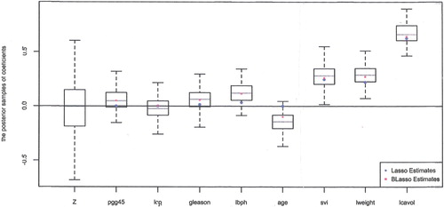
Figure 1 also includes Lasso and Bayesian Lasso estimates of each coefficients, marked as circles and squares in the figure. The Lasso estimates are zero for pgg45, lcp, and age, nonzero for the other 5 covariates. Thus, the Lasso approach agrees with our approach for covariates pgg45, lcp, age, svi, lweight, and lcavol, but does not agree on gleason and lbph. Since the magnitudes of Lasso estimates for gleason and lbph are small, another thresholding added to Lasso will result in the same conclusion with ours. Meanwhile, the Bayesian Lasso evaluates all the coefficients to be nonzero as it doesn't select variables to promote model sparsity.

Disclosure statement

No potential conflict of interest was reported by the authors.

References

- Brown, P. J., Vannucci, M., & Fearn, T. (1998). Multivariate Bayesian variable selection and prediction. Journal of the Royal Statistical Society, Series B, 60, 627–641. doi: 10.1111/1467-9868.00144
- Dellaportas, P., Forster, J. J., & I., Ntzoufras (1997). On Bayesian model and variable selection using MCMC (Technical Report). Athens: Department of Statistics, Athens University of Economics and Business.
- George, E. I., & McCulloch, R. E. (1993). Variable selection via Gibbs sampling. Journal of the American Statistical Association, 85, 398–409.
- Green, P. J. (1995). Reversible jump Markov chain Monte Carlo computation and Bayesian model determination. Biometrika, 82, 711–732. doi: 10.1093/biomet/82.4.711
- Griffin, J. E., & Brown, P. J. (2009). Inference with Normal-Gamma prior distributions in regression problems (Technical Report). Institute of Mathematics, Statistics and Actuarial Science, University of Kent.
- Hoti, F., & Sillanpää, M. J. (2006). Bayesian mapping of genotype x expression interactions in quantitative and qualitative traits. Heredity, 97, 4–18. doi: 10.1038/sj.hdy.6800817
- Kuo, L., & Mallick, B. (1998). Variable selection for regression models. Sankhya Series B, 60, 65–81.
- Kyung, M., Gilly, J., Ghosh, M., & Casella, G. (2010). Penalized regression, standard errors, and Bayesian Lassos. Bayesian Analysis, 5, 369–412. doi: 10.1214/10-BA607
- O'Hara, R. B., & Sillanpää, M. J. (2009). Review of Bayesian variable selection methods: What, how and which. Bayesian Analysis, 4, 85–118. doi: 10.1214/09-BA403
- Park, T., & Casella, G. (2008). The Bayesian Lasso. Journal of the American Statistical Association, 103, 681–686. doi: 10.1198/016214508000000337
- Stamey, T., Kabalin, J., McNeal, J., Johnstone, I., Freiha, F., Redwine, E., & Yang, N. (1989). Prostate specific antigen in the diagnosis and treatment of adenocarcinoma of the prostate. II. Radical prostatectomy treated patients. Journal of Urology, 141, 1076–1083. doi: 10.1016/S0022-5347(17)41175-X
- Tibshirani, R. (1996). Regression shrinkage and selection via the Lasso. Journal of the Royal Statistical Society, Series B, 58, 267–288.
- Tipping, M. (2001). Sparse Bayesian learning and the relevance vector machine. Journal of Machine Learning, 1, 211–244.
- Yuan, M., & Lin, Y. (2005). Efficient empirical Bayes variable selection and estimation in linear models. Journal of the American Statistical Association, 100, 1215–1225. doi: 10.1198/016214505000000367
- Zou, H., & Hastie, T. (2005). Regularization and variable selection via the elastic net. Journal of the Royal Statistical Society, Series B, 67, 301–320. doi: 10.1111/j.1467-9868.2005.00503.x