Interval estimation for minimal clinically important difference and its classification error via a bootstrap scheme

Abstract

With the improved knowledge on clinical relevance and more convenient access to the patient-reported outcome data, clinical researchers prefer to adopt minimal clinically important difference (MCID) rather than statistical significance as a testing standard to examine the effectiveness of certain intervention or treatment in clinical trials. A practical method to determining the MCID is based on the diagnostic measurement. By using this approach, the MCID can be formulated as the solution of a large margin classification problem. However, this method only produces the point estimation, hence lacks ways to evaluate its performance. In this paper, we introduce an m-out-of-n bootstrap approach which provides the interval estimations for MCID and its classification error, an associated accuracy measure for performance assessment. A variety of extensive simulation studies are implemented to show the advantages of our proposed method. Analysis of the chondral lesions and meniscus procedures (ChAMP) trial is our motivating example and is used to illustrate our method.

Keywords:

• Minimal clinically important difference
• classification error
• confidence interval
• non-convex optimisation
• bootstrap
• m-out-of-n bootstrap

1. Introduction

Statistical significance is widely reported in clinical studies to infer treatment effect. For instance, in a randomised controlled trial to compare debridement to the observation of chondral lesions encountered during partial meniscectomy (Bisson et al., 2017), the difference of the patient outcomes before surgery and one year after is used to assess the existence of any statistically significant effect.

Although this framework based on a threshold of the p-value objectifies the research outcome, solely relying on it can have two potentially serious consequences. First, statistical significance only signifies the existence of treatment effect, no matter how large is the effect size. The statistical significance could result from a huge sample size, hence may clinically irrelevant to the patients at all. Second, a clinically importance effect could be classified as statistically non-significant due to various reasons, say, the small sample size in the study, hence be unfairly ignored. In brief statistical significance does not necessarily imply clinical importance, and vice versa.

Over the years clinical investigators are realising that the determination of a treatment's clinical importance is much more valuable and reliable than merely seeking its statistical significance. Also, the development of various patient-rated instruments contributes huge amounts of patient-reported outcome (PRO) data, which provides the researchers with chances to study the clinical relevance. In order to study clinical importance, Jaeschke, Singer, and Guyatt (1989) proposed the concept of minimal clinically important difference (MCID). It is defined as the smallest change in an outcome that an individual patient would identify as important, therefore offers a threshold above which outcome is experienced as relevant by the patients. This avoids the problem of mere statistical significance (Wright, Hannon, Hegedus, & Kavchak, 2012). The MCID provides objective reference for clinicians and health policy-makers regarding the effectiveness of the treatment, hence has quickly gained its popularity (Erdogan, Leung, Pohl, Tennant, & Conaghan, 2016; McGlothlin & Lewis, 2014).

A variety of methods have been proposed to calculate the MCID. The anchor based method compares the changes in scores with an anchor as the reference. A popular anchor is the anchor question in the questionnaire. For instance, the short form (SF36) health survey (Ware & Sherbourne, 1992) serves this role in the ChAMP trial study (Bisson et al., 2017, 2018, 2019; Kluczynski et al., 2017). Hedayat, Wang, and Xu (2015) adopted this anchor based method and formulated the MCID as the threshold value in post-treatment change such that the probability of disagreement between the estimated satisfaction based on the MCID and the PRO is minimised.

Although the proposal in Hedayat et al. (2015) possesses the statistical rigour and paves the way for potential extension, it has some limitations. First, Hedayat et al. (2015) rely on a testing data set with a very large sample size to have their method implemented and assessed; however, the sample size of a clinical study is usually much smaller, therefore such a testing data set is not available for real application. Second, Hedayat et al. (2015) only provide a point estimation for the MCID, which is not informative enough in most clinical studies (Cook, 2008; Erdogan et al., 2016). Without an interval estimation, it is unknown how accurate this point estimation is. Furthermore, without an interval estimation, we have no idea how to compare multiple MCIDs derived for different population subgroups, hence the population heterogeneity could not be learned.

In this paper, we aim at solving the problems mentioned above and filling in this gap in the literature. We first introduce the concept of classification error to gauge the effectiveness of the MCID. More importantly, this concept also allows us to compare MCIDs derived for different population subgroups or computed using different methods. Second, using the m-out-of-n bootstrap technique, we obtain an interval estimation of the MCID, and also that of the classification error. The interval estimation makes it possible to conduct statistical inference on the MCID. It also allows us to fully learn the population heterogeneity based on the MCID.

Our proposal has two distinct features. First, different from Hedayat et al. (2015), our framework does not rely on a testing data set with a large sample size, hence can be conveniently used in various clinical studies. Second, although the bootstrap has already been a well-known and established statistical technique since Efron (1979), we stress that its conventional version cannot be directly applied in our context due to the restrictive conditions for it to be valid. Instead, the one we adopt is the m-out-of-n bootstrap with its theoretical properties justified in Shao (1994), Shao (1996), Bickel, Götze, and van Zwet (1997) and among others.

In the remainder of this paper, we first introduce our motivating example, the ChAMP trial study in Section 2. Then in Section 3, we review the concept of MCID and introduce that of the classification error. Our methodology, including both simple linear and nonparametric kernel MCIDs and the bootstrap scheme to compute the confidence interval, is presented in Section 4. We show the finite sample performance of our proposed method through simulation studies in Section 5 and apply our method to the ChAMP trial study in Section 6. The mathematical details are contained in Appendix.

2. Motivating example: ChAMP trial

Our motivating example is the chondral lesions and meniscus procedures (ChAMP) trial that examines whether the presence of the chondral lesions surrounding the knee cartilage affects patients' recovery from the arthroscopic partial meniscectomy (APM) (Bisson et al., 2017). In the field of orthopaedics, APM is one of the most common treatment options to repair the knee damage especially for the patients with a meniscus tear. During the operations, however, the surgeons can often find the additional knee damages in the form of chondral lesions. The effect of these chondral lesions on patients' post-operative outcomes are unclear, and whether these lesions need to be treated by debridement remains an open question. Thus, the ChAMP trial is designed to help the clinical physicians better understand this relation and provide them with reasonable suggestions on preoperative evaluation and treatment option.

This study enrolled eligible patients who were $\ge 30$ years old, diagnosed with a symptomatically consistent meniscus tear by magnetic resonance imaging, and underwent APM. Of the subjects who enrolled, 190 patients with surgically significant chondral lesions were randomised to receive debridement (CL-Deb group; n=98) or observation (CL-noDeb group; n=92). Outcome measures include the Western Ontario and McMaster Universities Osteoarthritis Index (WOMAC) and the SF-36 health survey. Each outcome was evaluated at baseline and one-year postoperatively. The demographic data such as age and sex at baseline and surgical data including the location and type of meniscal tears were also collected.

The major goal of the study is to assess whether and how the debridement group is different from the observation group in terms of the change of the WOMAC pain score from enrolment to one year after surgery, and how it relates to other covariate variables and clinical biomarkers. In our investigation, we focus on the study of the interval estimation of the MCID and its classification error. We use an anchor based method to compute the MCID and the anchor question we use is in the SF-36 health survey.

3. The MCID and the classification error

In the ChAMP trial, we denote each patient's reported outcome in the SF-36 health survey as a binary variable, where Y =1 if the patient reports a better health condition after the surgery and Y =−1 otherwise. The difference of each patient's WOMAC pain score from baseline to one year after surgery, denoted as X, is treated as the patient's diagnostic measurement. Let a p-dimensional covariate $\mathbf{Z}$ be the patient's clinical profile with $\mathbf{Z}\in {\mathcal{R}}^p$.

It is reasonable and of interest to consider the MCID $c^{\ast }$ as a function of the patient's clinical profile, $c^{\ast }\left(\mathbf{z}\right)$. The population heterogeneity could also be learned from the knowledge of $c^{\ast }\left(\mathbf{z}\right)$. According to Hedayat et al. (2015), the $c^{\ast }\left(\mathbf{z}\right)$ is defined as the minimiser of (1) $P[Y\ne \mathrm{s}\mathrm{i}\mathrm{g}\mathrm{n}\{X-c(\mathbf{Z}\left)\right\}]=\frac{1}{2}E[1-Y\mathrm{s}\mathrm{i}\mathrm{g}\mathrm{n}\{X-c(\mathbf{Z}\left)\right\}],$(1) where E is the expectation taken with respect to $(X,Y,\mathbf{Z})$ and $\mathrm{s}\mathrm{i}\mathrm{g}\mathrm{n}(\cdot )$ is the standard sign function. Given independent and identically distributed observations $\left\{\right(x_i,y_i,{\mathbf{z}}_i),i=1,\dots ,n\}$, the empirical version of the objective function in (1(1) $P[Y\ne \mathrm{s}\mathrm{i}\mathrm{g}\mathrm{n}\{X-c(\mathbf{Z}\left)\right\}]=\frac{1}{2}E[1-Y\mathrm{s}\mathrm{i}\mathrm{g}\mathrm{n}\{X-c(\mathbf{Z}\left)\right\}],$(1) ) becomes (2) $\frac{1}{2n}\sum _{i=1}^n\left[1-y_i\mathrm{s}\mathrm{i}\mathrm{g}\mathrm{n}\{x_i-c({\mathbf{z}}_i\left)\right\}\right],$(2) which involves the 0–1 loss function $L_{01}\left(u\right)=\frac{1}{2}(1-\mathrm{s}\mathrm{i}\mathrm{g}\mathrm{n}(u\left)\right)$. The direct minimisation of (2(2) $\frac{1}{2n}\sum _{i=1}^n\left[1-y_i\mathrm{s}\mathrm{i}\mathrm{g}\mathrm{n}\{x_i-c({\mathbf{z}}_i\left)\right\}\right],$(2) ) is infeasible. In this paper, we follow Hedayat et al. (2015) to approximate the $L_{01}$ function with the non-smooth ramp loss function. Note that the non-smooth ramp loss is defined as $L_{\delta }\left(u\right)=\left\{\begin{array}{ll}1& u\le 0,\\ 1-\frac{u}{\delta }& 0<u\le \delta ,\\ 0& u>\delta ,\end{array}\right.$ where $\delta >0$ is a scalar factor. As $\delta \to 0$, $L_{\delta }(\cdot )\to L_{01}(\cdot )$. Then our objective function becomes (3) $\frac{1}{n}\sum _{i=1}^n{L}_{\delta }\left\{y_i\right(x_i-c\left({\mathbf{z}}_i\right)\left)\right\}.$(3) Due to the non-convexity of the non-smooth ramp loss, the optimisation problem in (3(3) $\frac{1}{n}\sum _{i=1}^n{L}_{\delta }\left\{y_i\right(x_i-c\left({\mathbf{z}}_i\right)\left)\right\}.$(3) ) requires nonconvex minimisation. Note that we can write $L_{\delta }\left(u\right)=L_1\left(u\right)-L_2\left(u\right)$, where both $L_1\left(u\right)=\left(1/\delta \right)(\delta -u{)}_{+}$ and $L_2\left(u\right)=\left(1/\delta \right)(-u{)}_{+}$ are convex functions. Hence, we apply the difference of convex (DC) algorithm (ThiHoaiAn & DinhTao, 1997) to minimise (3(3) $\frac{1}{n}\sum _{i=1}^n{L}_{\delta }\left\{y_i\right(x_i-c\left({\mathbf{z}}_i\right)\left)\right\}.$(3) ), which has the form (4) $\frac{1}{n}\sum _{i=1}^n{L}_1\left\{y_i\right(x_i-c\left({\mathbf{z}}_i\right)\left)\right\}-\frac{1}{n}\sum _{i=1}^n{L}_2\left\{y_i\right(x_i-c\left({\mathbf{z}}_i\right)\left)\right\}.$(4) Figure 1 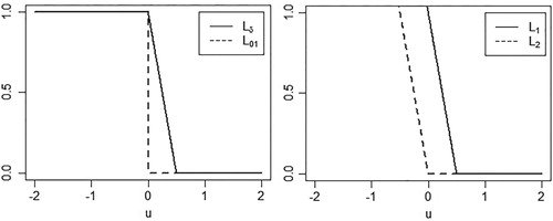illustrates the relation among the $L_{01}$, $L_{\delta }$, $L_1$ and $L_2$ loss functions.

Figure 1. The illustration of the 0–1 loss $L_{01}$, its surrogate non-smooth ramp loss $L_{\delta }$, and the DC decomposition $L_{\delta }=L_1-L_2$.

Once the minimiser $\hat{c}$ is obtained, we can validate whether the debridement or the observation of the chondral lesions for each patient is indeed prescribed correctly. This is essential since it provides knowledgeable advice in future surgical practice for new patients. To re-evaluate whether the treatment is offered appropriately, we need a statistical measure to quantify the discrepancy between the patient's PRO $Y_0$ and its dichotomous diagnostic measure from learning his/her MCID $\mathrm{s}\mathrm{i}\mathrm{g}\mathrm{n}\{X_0-c({\mathbf{Z}}_0\left)\right\}$. Here, to avoid confusion, we use a generic notation $\left\{\right(Y_0,X_0,{\mathbf{Z}}_0\left)\right\}$ to represent any patient that would like to be validated. This results in (5) $E_0[\text{𝟙}\{Y_0\ne \mathrm{s}\mathrm{i}\mathrm{g}\mathrm{n}\{X_0-\hat{c}({\mathbf{Z}}_0\left)\right\}\}],$(5) where $E_0$ is the expectation taken with respect to $\left\{\right(Y_0,X_0,{\mathbf{Z}}_0\left)\right\}$. While there are other alternative measures to study, this error (5(5) $E_0[\text{𝟙}\{Y_0\ne \mathrm{s}\mathrm{i}\mathrm{g}\mathrm{n}\{X_0-\hat{c}({\mathbf{Z}}_0\left)\right\}\}],$(5) ), usually called the classification error, or the test error, is popularly used in the statistical machine learning literature.

The estimation for the classification error is not a trivial task (Laber & Murphy, 2011). In this paper, we concentrate on creating confidence intervals for both the MCID and the classification error.

4. Methodology

In this section, we first present detailed algorithms to calculating MCID. We consider both simple linear MCID and its nonparametric kernel counterpart. We then introduce our bootstrap scheme to construct confidence intervals for MCID and the classification error.

4.1. Algorithms for MCID

It is of particular interest to clinicians if the MCID has a comprehensible structure. For instance, $c\left(\mathbf{Z}\right)=\alpha +{\text{β}}^{\mathrm{T}}\mathbf{Z}$, where $\mathbf{Z}$ could include the treatment variable, some of the demographic variables and clinical biomarkers. This is the simple linear MCID we consider below. On the other hand, although easily interpretable, a linear structure suffers from the model misspecification issue, thereby yields a solution which may not achieve optimal performance. Therefore, we also consider the nonparametric kernel MCID adopting the reproducing kernel Hilbert space framework.

4.1.1. A simple linear MCID

We assume $c\left(\mathbf{Z}\right)=\alpha +{\text{β}}^{\mathrm{T}}\mathbf{Z}$. We add a penalty term $\left(\lambda /2\right){\text{β}}^{\mathrm{T}}\text{β}$ in (4(4) $\frac{1}{n}\sum _{i=1}^n{L}_1\left\{y_i\right(x_i-c\left({\mathbf{z}}_i\right)\left)\right\}-\frac{1}{n}\sum _{i=1}^n{L}_2\left\{y_i\right(x_i-c\left({\mathbf{z}}_i\right)\left)\right\}.$(4) ) to avoid model overfitting. Let $\mathit{\omega }=(\alpha ,{\text{β}}^{\mathrm{T}}{)}^{\mathrm{T}}$, then the objective function in (4(4) $\frac{1}{n}\sum _{i=1}^n{L}_1\left\{y_i\right(x_i-c\left({\mathbf{z}}_i\right)\left)\right\}-\frac{1}{n}\sum _{i=1}^n{L}_2\left\{y_i\right(x_i-c\left({\mathbf{z}}_i\right)\left)\right\}.$(4) ) is $s\left(\mathit{\omega }\right)=s_1\left(\mathit{\omega }\right)-s_2\left(\mathit{\omega }\right)$, where $\begin{array}{rl}{s}_1\left(\mathit{\omega }\right)& =\frac{1}{n}\sum _{i=1}^n\left[\frac{1}{\delta }\{\delta -y_i(x_i-\alpha -{\text{β}}^{\mathrm{T}}{\mathbf{z}}_i){\}}_{+}\right]+\frac{\lambda }{2}{\text{β}}^{\mathrm{T}}\text{β},\\ s_2\left(\mathit{\omega }\right)& =\frac{1}{n}\sum _{i=1}^n\left[\frac{1}{\delta }\{-y_i(x_i-\alpha -{\text{β}}^{\mathrm{T}}{\mathbf{z}}_i){\}}_{+}\right].\end{array}$ It is an iterative algorithm to minimise (4(4) $\frac{1}{n}\sum _{i=1}^n{L}_1\left\{y_i\right(x_i-c\left({\mathbf{z}}_i\right)\left)\right\}-\frac{1}{n}\sum _{i=1}^n{L}_2\left\{y_i\right(x_i-c\left({\mathbf{z}}_i\right)\left)\right\}.$(4) ). Let ${\hat{\mathit{\omega }}}^{\left(k\right)}$ be the estimator of $\mathit{\omega }$ at the kth iteration. We first approximate $s_2\left(\mathit{\omega }\right)$ with its affine minorisation function $s_2\left({\hat{\mathit{\omega }}}^{\left(k\right)}\right)+⟨\mathit{\omega }-{\hat{\mathit{\omega }}}^{\left(k\right)},\mathrm{\nabla }{s}_2\left({\hat{\mathit{\omega }}}^{\left(k\right)}\right)⟩$, where $\mathrm{\nabla }{s}_2\left({\hat{\mathit{\omega }}}^{\left(k\right)}\right)$ is the subgradient of $s_2\left(\mathit{\omega }\right)$ at ${\hat{\mathit{\omega }}}^{\left(k\right)}$, $\mathrm{\nabla }{s}_2\left({\hat{\mathit{\omega }}}^{\left(k\right)}\right)=\left(\begin{array}{c}\begin{array}{c}\frac{1}{n\delta }\sum _{i=1}^n{y}_i\text{𝟙}\{y_i(x_i-{\alpha }^{\left(k\right)}\\ -{\text{β}}^{\left(k\right)\mathrm{T}}{\mathbf{z}}_i)<0\}\end{array}\\ \begin{array}{c}\frac{1}{n\delta }\sum _{i=1}^n{y}_i{\mathbf{z}}_i\text{𝟙}\{y_i(x_i-{\alpha }^{\left(k\right)}\\ -{\text{β}}^{\left(k\right)\mathrm{T}}{\mathbf{z}}_i)<0\}\end{array}\end{array}\right).$ Hence (6) $\begin{array}{rl}{\hat{\mathit{\omega }}}^{(k+1)}& ={\mathrm{a}\mathrm{r}\mathrm{g}\mathrm{m}\mathrm{i}\mathrm{n}}_{\mathit{\omega }}{s}_1\left(\mathit{\omega }\right)-{\mathit{\omega }}^{\mathrm{T}}\mathrm{\nabla }{s}_2\left({\hat{\mathit{\omega }}}^{\left(k\right)}\right),\\ & ={\mathrm{a}\mathrm{r}\mathrm{g}\mathrm{m}\mathrm{i}\mathrm{n}}_{\mathit{\omega }}{s}_1\left(\mathit{\omega }\right)\\ & -\frac{1}{n\delta }\sum _{i=1}^n{y}_i(\alpha +{\text{β}}^{\mathrm{T}}{\mathbf{z}}_i)\text{𝟙}\\ & \{y_i(x_i-{\alpha }^{\left(k\right)}-{\text{β}}^{\left(k\right)\mathrm{T}}{\mathbf{z}}_i)<0\}.\end{array}$(6)

To solve (6(6) $\begin{array}{rl}{\hat{\mathit{\omega }}}^{(k+1)}& ={\mathrm{a}\mathrm{r}\mathrm{g}\mathrm{m}\mathrm{i}\mathrm{n}}_{\mathit{\omega }}{s}_1\left(\mathit{\omega }\right)-{\mathit{\omega }}^{\mathrm{T}}\mathrm{\nabla }{s}_2\left({\hat{\mathit{\omega }}}^{\left(k\right)}\right),\\ & ={\mathrm{a}\mathrm{r}\mathrm{g}\mathrm{m}\mathrm{i}\mathrm{n}}_{\mathit{\omega }}{s}_1\left(\mathit{\omega }\right)\\ & -\frac{1}{n\delta }\sum _{i=1}^n{y}_i(\alpha +{\text{β}}^{\mathrm{T}}{\mathbf{z}}_i)\text{𝟙}\\ & \{y_i(x_i-{\alpha }^{\left(k\right)}-{\text{β}}^{\left(k\right)\mathrm{T}}{\mathbf{z}}_i)<0\}.\end{array}$(6) ), we derive its dual problem by using the slack variable technique. The details are retained in Appendix 1. It shows that, we arrive at the dual problem (7) $\underset{\mathit{\tau }}{min}{\mathit{\tau }}^{\mathrm{T}}\mathbf{Q}\mathit{\tau }-\{\mathbf{b}+2\mathbf{Q}{\mathbf{t}}_1({\alpha }^{\left(k\right)},{\text{β}}^{\left(k\right)}){\}}^{\mathrm{T}}\mathit{\tau },$(7) subject to $0\le {\tau }_i\le 1$ and $\sum _{i=1}^n\left(1/\delta \right)y_i\{{\tau }_i-t_{1,i}({\alpha }^{\left(k\right)},{\text{β}}^{\left(k\right)}\left)\right\}=0$. This optimisation problem only has simple box constraints hence can be solved by any quadratic programming method.

We conclude the algorithm by presenting how $\hat{\alpha }$ and $\widehat{\text{β}}$ can be computed. The Karush–Kuhn–Tucker (KKT) conditions associated with optimisation problem (7(7) $\underset{\mathit{\tau }}{min}{\mathit{\tau }}^{\mathrm{T}}\mathbf{Q}\mathit{\tau }-\{\mathbf{b}+2\mathbf{Q}{\mathbf{t}}_1({\alpha }^{\left(k\right)},{\text{β}}^{\left(k\right)}){\}}^{\mathrm{T}}\mathit{\tau },$(7) ) are, respectively, (8) $\begin{array}{rl}\frac{1}{n\lambda \delta }\sum _{i=1}^n{y}_i\{t_{1,i}({\alpha }^{\left(k\right)},{\text{β}}^{\left(k\right)})-{\tau }_i\}{\mathbf{z}}_i& =\text{β},\end{array}$(8) (9) $\begin{array}{rl}1& \ge {\tau }_i\ge 0,\end{array}$(9) (10) $\begin{array}{rl}{\tau }_i\left\{{\xi }_i-1+\frac{1}{\delta }{y}_i(x_i-\alpha -{\text{β}}^{\mathrm{T}}{\mathbf{z}}_i)\right\}& =0,\end{array}$(10) (11) $\begin{array}{rl}{\xi }_i& \ge 0,\end{array}$(11) (12) $\begin{array}{rl}{\xi }_i-1+\frac{1}{\delta }{y}_i(x_i-\alpha -{\text{β}}^{\mathrm{T}}{\mathbf{z}}_i)& \ge 0,\end{array}$(12) (13) $\begin{array}{rl}(1-{\tau }_i){\xi }_i& =0.\end{array}$(13) Therefore, we have three scenarios to discuss depending on the magnitude of ${\tau }_i$: if ${\tau }_i=0$, by (12(12) $\begin{array}{rl}{\xi }_i-1+\frac{1}{\delta }{y}_i(x_i-\alpha -{\text{β}}^{\mathrm{T}}{\mathbf{z}}_i)& \ge 0,\end{array}$(12) ) and (13(13) $\begin{array}{rl}(1-{\tau }_i){\xi }_i& =0.\end{array}$(13) ) we get ${\xi }_i=0$ and $\left(1/\delta \right)y_i(x_i-\alpha -{\text{β}}^{\mathrm{T}}{\mathbf{z}}_i)-1\ge 0$; if $1>{\tau }_i>0$, by (10(10) $\begin{array}{rl}{\tau }_i\left\{{\xi }_i-1+\frac{1}{\delta }{y}_i(x_i-\alpha -{\text{β}}^{\mathrm{T}}{\mathbf{z}}_i)\right\}& =0,\end{array}$(10) ) and (13(13) $\begin{array}{rl}(1-{\tau }_i){\xi }_i& =0.\end{array}$(13) ) we have ${\xi }_i=0$ and $\left(1/\delta \right)y_i(x_i-\alpha -{\text{β}}^{\mathrm{T}}{\mathbf{z}}_i)-1=0$; if ${\tau }_i=1$, by (10(10) $\begin{array}{rl}{\tau }_i\left\{{\xi }_i-1+\frac{1}{\delta }{y}_i(x_i-\alpha -{\text{β}}^{\mathrm{T}}{\mathbf{z}}_i)\right\}& =0,\end{array}$(10) ), (12(12) $\begin{array}{rl}{\xi }_i-1+\frac{1}{\delta }{y}_i(x_i-\alpha -{\text{β}}^{\mathrm{T}}{\mathbf{z}}_i)& \ge 0,\end{array}$(12) ) and (13(13) $\begin{array}{rl}(1-{\tau }_i){\xi }_i& =0.\end{array}$(13) ) we have $\left(1/\delta \right)y_i(x_i-\alpha -{\text{β}}^{\mathrm{T}}{\mathbf{z}}_i)-1=-{\xi }_i\le 0$. Therefore, we can summarise the KKT conditions more concisely as $\begin{array}{rl}\frac{1}{\delta }{y}_i(x_i-\alpha -{\text{β}}^{\mathrm{T}}{\mathbf{z}}_i)-1& =-{\xi }_i\ge 0\mathrm{i}\mathrm{f}{\tau }_i<1,\\ \frac{1}{\delta }{y}_i(x_i-\alpha -{\text{β}}^{\mathrm{T}}{\mathbf{z}}_i)-1& =-{\xi }_i\le 0\mathrm{i}\mathrm{f}{\tau }_i>0,\end{array}$ which implies (14) $\frac{1}{\delta }{y}_i(x_i-\alpha -{\text{β}}^{\mathrm{T}}{\mathbf{z}}_i)-1=0\mathrm{i}\mathrm{f}0<{\tau }_i<1.$(14) Hence through (8(8) $\begin{array}{rl}\frac{1}{n\lambda \delta }\sum _{i=1}^n{y}_i\{t_{1,i}({\alpha }^{\left(k\right)},{\text{β}}^{\left(k\right)})-{\tau }_i\}{\mathbf{z}}_i& =\text{β},\end{array}$(8) ) we can estimate ${\text{β}}^{(k+1)}$ as ${\widehat{\text{β}}}^{(k+1)}=\frac{1}{n\lambda \delta }\sum _{i=1}^n{y}_i\{t_{1,i}({\alpha }^{\left(k\right)},{\text{β}}^{\left(k\right)})-{\hat{\tau }}_i\}{\mathbf{z}}_i,$ and through (14(14) $\frac{1}{\delta }{y}_i(x_i-\alpha -{\text{β}}^{\mathrm{T}}{\mathbf{z}}_i)-1=0\mathrm{i}\mathrm{f}0<{\tau }_i<1.$(14) ) we can estimate ${\alpha }^{(k+1)}$ as $\begin{array}{rl}& {\hat{\alpha }}^{(k+1)}=\frac{1}{|\{i:0<{\tau }_i<1\}|}\\ & \sum _{i:0<{\tau }_i<1}\left(x_i-\frac{\delta }{y_i}-{\widehat{\text{β}}}^{(k+1)\mathrm{T}}{\mathbf{z}}_i\right).\end{array}$ Finally, we achieve the estimators $\hat{\alpha }$ and $\widehat{\text{β}}$ after iterative process (6(6) $\begin{array}{rl}{\hat{\mathit{\omega }}}^{(k+1)}& ={\mathrm{a}\mathrm{r}\mathrm{g}\mathrm{m}\mathrm{i}\mathrm{n}}_{\mathit{\omega }}{s}_1\left(\mathit{\omega }\right)-{\mathit{\omega }}^{\mathrm{T}}\mathrm{\nabla }{s}_2\left({\hat{\mathit{\omega }}}^{\left(k\right)}\right),\\ & ={\mathrm{a}\mathrm{r}\mathrm{g}\mathrm{m}\mathrm{i}\mathrm{n}}_{\mathit{\omega }}{s}_1\left(\mathit{\omega }\right)\\ & -\frac{1}{n\delta }\sum _{i=1}^n{y}_i(\alpha +{\text{β}}^{\mathrm{T}}{\mathbf{z}}_i)\text{𝟙}\\ & \{y_i(x_i-{\alpha }^{\left(k\right)}-{\text{β}}^{\left(k\right)\mathrm{T}}{\mathbf{z}}_i)<0\}.\end{array}$(6) ) converges. For any new patient with data ${\mathbf{z}}_{\mathrm{n}\mathrm{e}\mathrm{w}}$, his/her predicted linear MCID is $\hat{c}\left({\mathbf{z}}_{\mathrm{n}\mathrm{e}\mathrm{w}}\right)=\hat{\alpha }+{\widehat{\text{β}}}^{\mathrm{T}}{\mathbf{z}}_{\mathrm{n}\mathrm{e}\mathrm{w}}.$

4.1.2. A nonparametric kernel MCID

Define a feature vector ${\mathit{\phi }}_i=\phi \left({\mathbf{z}}_i\right)$ for the profiles of the ith patient in the enlarged feature space. We can specify a continuous, symmetric and positive-semidefinite kernel function K corresponding to the inner product in the mapping φ, that is, $K({\mathbf{z}}_i,{\mathbf{z}}_j)=⟨{\mathit{\phi }}_i,{\mathit{\phi }}_j⟩$. Then, we have $c\left(\mathbf{z}\right)=w+h\left(\mathbf{z}\right)$ with $w\in \mathcal{R}$ and $h\left(\mathbf{z}\right)\in {\mathcal{H}}_K$, where ${\mathcal{H}}_K$ is the reproducing kernel Hilbert space (RKHS) with a kernel function $K(\cdot ,\cdot )$. The norm in ${\mathcal{H}}_K$, denoted by $||\cdot |{|}_K$, is induced by the following inner product: $⟨f,g{⟩}_K=\sum _{i=1}^n\sum _{j=1}^m{v}_i{u}_{j}K({\mathbf{z}}_i,{\mathbf{z}}_j),$ where $f(\cdot )=\sum _{i=1}^n{v}_{i}K(\cdot ,{\mathbf{z}}_i)$ and $g(\cdot )=\sum _{j=1}^m{u}_{j}K(\cdot ,{\mathbf{z}}_j)$.

Following the representation theorem (Kimeldorf & Wahba, 1971), the nonparametric kernel MCID can be expressed as $c\left(\mathbf{z}\right)=w+\sum _{j=1}^n{v}_{j}K(\mathbf{z},{\mathbf{z}}_j)$. Let $\mathit{\eta }=(w,{\mathit{v}}^{\mathrm{T}}{)}^{\mathrm{T}}=(w,v_1,\dots ,v_n{)}^{\mathrm{T}}$, then the objective function in (4(4) $\frac{1}{n}\sum _{i=1}^n{L}_1\left\{y_i\right(x_i-c\left({\mathbf{z}}_i\right)\left)\right\}-\frac{1}{n}\sum _{i=1}^n{L}_2\left\{y_i\right(x_i-c\left({\mathbf{z}}_i\right)\left)\right\}.$(4) ) is $h\left(\mathit{\eta }\right)=h_1\left(\mathit{\eta }\right)-h_2\left(\mathit{\eta }\right)$, where $\begin{array}{rl}{h}_1\left(\mathit{\eta }\right)& =\frac{1}{n}\sum _{i=1}^n\left[\frac{1}{\delta }\left\{\delta -y_i\left(x_i-w\right.\right.\right.\\ & \left.{\left.\left.-\sum _{j=1}^n{v}_{j}K({\mathbf{z}}_i,{\mathbf{z}}_j)\right)\right\}}_{+}\right]+\frac{\lambda }{2}\sum _{i,j=1}^n{v}_i{v}_{j}K({\mathbf{z}}_i,{\mathbf{z}}_j),\\ h_2\left(\mathit{\eta }\right)& =\frac{1}{n}\sum _{i=1}^n\left[\frac{1}{\delta }\left\{-y_i\left(x_i-w\right.\right.\right.\\ & \left.{\left.\left.-\sum _{j=1}^n{v}_{j}K({\mathbf{z}}_i,{\mathbf{z}}_j)\right)\right\}}_{+}\right].\end{array}$ Similar to the linear case, it is an iterative algorithm to minimise  (4(4) $\frac{1}{n}\sum _{i=1}^n{L}_1\left\{y_i\right(x_i-c\left({\mathbf{z}}_i\right)\left)\right\}-\frac{1}{n}\sum _{i=1}^n{L}_2\left\{y_i\right(x_i-c\left({\mathbf{z}}_i\right)\left)\right\}.$(4) ). Let ${\hat{\mathit{\eta }}}^{\left(k\right)}$ be the estimator of $\mathit{\eta }$ at the $k^{th}$ iteration. We first approximate $h_2\left(\mathit{\eta }\right)$ with its affine minorisation function $h_2\left({\hat{\mathit{\eta }}}^{\left(k\right)}\right)+⟨\mathit{\eta }-{\hat{\mathit{\eta }}}^{\left(k\right)},\mathrm{\nabla }{h}_2\left({\hat{\mathit{\eta }}}^{\left(k\right)}\right)⟩$, where $\mathrm{\nabla }{h}_2\left({\hat{\mathit{\eta }}}^{\left(k\right)}\right)$ is the subgradient of $h_2\left(\mathit{\eta }\right)$ at ${\hat{\mathit{\eta }}}^{\left(k\right)}$, $\mathrm{\nabla }{h}_2\left({\hat{\mathit{\eta }}}^{\left(k\right)}\right)=\left(\begin{array}{c}\frac{1}{n\delta }\sum _{i=1}^n{y}_i\text{𝟙}\left\{y_i(x_i-w^{\left(k\right)}\right.\\ \left.-\sum _{j=1}^n{v}_j^{\left(k\right)}K({\mathbf{z}}_i,{\mathbf{z}}_j))<0\right\}\\ \frac{1}{n\delta }\sum _{i=1}^n{y}_{i}K({\mathbf{z}}_i,{\mathbf{z}}_1)\text{𝟙}\left\{y_i(x_i-w^{\left(k\right)}\right.\\ \left.-\sum _{j=1}^n{v}_j^{\left(k\right)}K({\mathbf{z}}_i,{\mathbf{z}}_j))<0\right\}\\ ⋮\\ \frac{1}{n\delta }\sum _{i=1}^n{y}_{i}K({\mathbf{z}}_i,{\mathbf{z}}_n)\text{𝟙}\left\{y_i(x_i-w^{\left(k\right)}\right.\\ \left.-\sum _{j=1}^n{v}_j^{\left(k\right)}K({\mathbf{z}}_i,{\mathbf{z}}_j))<0\right\}\end{array}\right).$ Consequently, (15) $\begin{array}{rl}& {\hat{\mathit{\eta }}}^{(k+1)}={\mathrm{a}\mathrm{r}\mathrm{g}\mathrm{m}\mathrm{i}\mathrm{n}}_{\mathit{\eta }}{h}_1\left(\mathit{\eta }\right)-{\mathit{\eta }}^{\mathrm{T}}\mathrm{\nabla }{h}_2\left({\hat{\mathit{\eta }}}^{\left(k\right)}\right),\\ & ={\mathrm{a}\mathrm{r}\mathrm{g}\mathrm{m}\mathrm{i}\mathrm{n}}_{\mathit{\eta }}{h}_1\left(\mathit{\eta }\right)-\frac{1}{n\delta }\sum _{i=1}^n{y}_i(w\\ & +\sum _{j=1}^n{v}_{j}K({\mathbf{z}}_i,{\mathbf{z}}_j))\text{𝟙}\left\{y_i(x_i-w^{\left(k\right)}\right.\\ & \left.-\sum _{j=1}^n{v}_j^{\left(k\right)}K({\mathbf{z}}_i,{\mathbf{z}}_j))<0\right\}.\end{array}$(15)

Similar to the linear case, we use the slack variable technique and reach the dual problem (16) $\underset{{\mathit{\tau }}^{\mathrm{\prime }}}{min}{\mathit{\tau }}^{\mathrm{\prime }T}{\mathbf{Q}}^{\mathrm{\prime }}{\mathit{\tau }}^{\mathrm{\prime }}-\{\mathbf{d}+2{\mathbf{Q}}^{\mathrm{\prime }}{\mathbf{t}}_2(w^{\left(k\right)},{\mathit{v}}^{\left(k\right)}){\}}^{\mathrm{T}}{\mathit{\tau }}^{\mathrm{\prime }},$(16) subject to $0\le {\tau }_i^{\mathrm{\prime }}\le 1$ and $\sum _{i=1}^n\left(1/\delta \right)y_i\{{\tau }_i^{\mathrm{\prime }}-t_{2,i}(w^{\left(k\right)},{\mathit{v}}^{\left(k\right)}\left)\right\}=0$. This optimisation problem only have simple box constraints hence can be solved by any quadratic programming method.

We conclude the algorithm by presenting how $\hat{w}$ and $\hat{\mathit{v}}$ can be computed. The Karush–Kuhn–Tucker (KKT) conditions associated with optimisation problem (16(16) $\underset{{\mathit{\tau }}^{\mathrm{\prime }}}{min}{\mathit{\tau }}^{\mathrm{\prime }T}{\mathbf{Q}}^{\mathrm{\prime }}{\mathit{\tau }}^{\mathrm{\prime }}-\{\mathbf{d}+2{\mathbf{Q}}^{\mathrm{\prime }}{\mathbf{t}}_2(w^{\left(k\right)},{\mathit{v}}^{\left(k\right)}){\}}^{\mathrm{T}}{\mathit{\tau }}^{\mathrm{\prime }},$(16) ) are, respectively, (17) $\begin{array}{rl}& \frac{1}{n\lambda \delta }{y}_i\{t_{2,i}(w^{\left(k\right)},{\mathit{v}}^{\left(k\right)})-{\tau }_i^{\mathrm{\prime }}\}{\mathit{\phi }}_i=v_i,\end{array}$(17) (18) $\begin{array}{rl}& 1\ge {\tau }_i^{\mathrm{\prime }}\ge 0,\end{array}$(18) (19) $\begin{array}{rl}& {\tau }_i^{\mathrm{\prime }}\left\{{\xi }_i^{\mathrm{\prime }}-1+\frac{1}{\delta }{y}_i\left(x_i-w-\sum _{j=1}^n{v}_{j}K\left({\mathbf{z}}_i,{\mathbf{z}}_j\right)\right)\right\}=0,\end{array}$(19) (20) $\begin{array}{rl}& {\xi }_i^{\mathrm{\prime }}\ge 0,\end{array}$(20) (21) $\begin{array}{rl}& {\xi }_i^{\mathrm{\prime }}-1+\frac{1}{\delta }{y}_i\left(x_i-w-\sum _{j=1}^n{v}_{j}K\left({\mathbf{z}}_i,{\mathbf{z}}_j\right)\right)\ge 0,\end{array}$(21) (22) $\begin{array}{rl}& (1-{\tau }_i^{\mathrm{\prime }}){\xi }_i^{\mathrm{\prime }}=0.\end{array}$(22) Three scenarios can be consequently discussed based on the magnitude of ${\tau }_i^{\mathrm{\prime }}$: if ${\tau }_i^{\mathrm{\prime }}=0$, by (21(21) $\begin{array}{rl}& {\xi }_i^{\mathrm{\prime }}-1+\frac{1}{\delta }{y}_i\left(x_i-w-\sum _{j=1}^n{v}_{j}K\left({\mathbf{z}}_i,{\mathbf{z}}_j\right)\right)\ge 0,\end{array}$(21) ) and (22(22) $\begin{array}{rl}& (1-{\tau }_i^{\mathrm{\prime }}){\xi }_i^{\mathrm{\prime }}=0.\end{array}$(22) ) we have ${\xi }_i^{\mathrm{\prime }}=0$ and $\left(1/\delta \right)y_i(x_i-w-\sum _{j=1}^n{v}_{j}K({\mathbf{z}}_i,{\mathbf{z}}_j\left)\right)-1\ge 0$; if $1>{\tau }_i^{\mathrm{\prime }}>0$, by (19(19) $\begin{array}{rl}& {\tau }_i^{\mathrm{\prime }}\left\{{\xi }_i^{\mathrm{\prime }}-1+\frac{1}{\delta }{y}_i\left(x_i-w-\sum _{j=1}^n{v}_{j}K\left({\mathbf{z}}_i,{\mathbf{z}}_j\right)\right)\right\}=0,\end{array}$(19) ) and (22(22) $\begin{array}{rl}& (1-{\tau }_i^{\mathrm{\prime }}){\xi }_i^{\mathrm{\prime }}=0.\end{array}$(22) ) we obtain ${\xi }_i^{\mathrm{\prime }}=0$ and $\left(1/\delta \right)y_i(x_i-w-\sum _{j=1}^n{v}_{j}K({\mathbf{z}}_i,{\mathbf{z}}_j\left)\right)-1=0$; if ${\tau }_i^{\mathrm{\prime }}=1$, by (19(19) $\begin{array}{rl}& {\tau }_i^{\mathrm{\prime }}\left\{{\xi }_i^{\mathrm{\prime }}-1+\frac{1}{\delta }{y}_i\left(x_i-w-\sum _{j=1}^n{v}_{j}K\left({\mathbf{z}}_i,{\mathbf{z}}_j\right)\right)\right\}=0,\end{array}$(19) ), (21(21) $\begin{array}{rl}& {\xi }_i^{\mathrm{\prime }}-1+\frac{1}{\delta }{y}_i\left(x_i-w-\sum _{j=1}^n{v}_{j}K\left({\mathbf{z}}_i,{\mathbf{z}}_j\right)\right)\ge 0,\end{array}$(21) ) and (22(22) $\begin{array}{rl}& (1-{\tau }_i^{\mathrm{\prime }}){\xi }_i^{\mathrm{\prime }}=0.\end{array}$(22) ) we obtain $\left(1/\delta \right)y_i(x_i-w-\sum _{j=1}^n{v}_{j}K({\mathbf{z}}_i,{\mathbf{z}}_j\left)\right)-1=-{\xi }_i^{\mathrm{\prime }}\le 0$. Now we can summarise the KKT conditions more concisely as $\begin{array}{rl}& \frac{1}{\delta }{y}_i\left(x_i-w-\sum _{j=1}^n{v}_{j}K\left({\mathbf{z}}_i,{\mathbf{z}}_j\right)\right)-1=-{\xi }_i^{\mathrm{\prime }}\ge 0\\ & \mathrm{i}\mathrm{f}{\tau }_i^{\mathrm{\prime }}<1,\\ & \frac{1}{\delta }{y}_i\left(x_i-w-\sum _{j=1}^n{v}_{j}K\left({\mathbf{z}}_i,{\mathbf{z}}_j\right)\right)-1=-{\xi }_i^{\mathrm{\prime }}\le 0\\ & \mathrm{i}\mathrm{f}{\tau }_i^{\mathrm{\prime }}>0,\end{array}$ which implies (23) $\frac{1}{\delta }{y}_i\left(x_i-w-\sum _{j=1}^n{v}_{j}K\left({\mathbf{z}}_i,{\mathbf{z}}_j\right)\right)-1=0\mathrm{i}\mathrm{f}0<{\tau }_i^{\mathrm{\prime }}<1.$(23) Thus for $i=1,\dots ,n$, $v_i^{(k+1)}$ can be estimated via (17(17) $\begin{array}{rl}& \frac{1}{n\lambda \delta }{y}_i\{t_{2,i}(w^{\left(k\right)},{\mathit{v}}^{\left(k\right)})-{\tau }_i^{\mathrm{\prime }}\}{\mathit{\phi }}_i=v_i,\end{array}$(17) ) as ${\hat{v}}_i^{(k+1)}=\frac{1}{n\lambda \delta }{y}_i\{t_{2,i}(w^{\left(k\right)},{\mathit{v}}^{\left(k\right)})-{\hat{\tau }}_i^{\mathrm{\prime }}\}{\mathit{\phi }}_i$ and $w^{(k+1)}$ can be estimated via (23(23) $\frac{1}{\delta }{y}_i\left(x_i-w-\sum _{j=1}^n{v}_{j}K\left({\mathbf{z}}_i,{\mathbf{z}}_j\right)\right)-1=0\mathrm{i}\mathrm{f}0<{\tau }_i^{\mathrm{\prime }}<1.$(23) ) as $\begin{array}{rl}{\hat{w}}^{(k+1)}& =\frac{1}{|\{i:0<{\tau }_i^{\mathrm{\prime }}<1\}|}\\ & \sum _{i:0<{\tau }_i^{\mathrm{\prime }}<1}\left(x_i-\frac{\delta }{y_i}-\sum _{j=1}^n{\hat{v}}_{j}K\left({\mathbf{z}}_i,{\mathbf{z}}_j\right)\right).\end{array}$ We can get the estimators $\hat{w}$ and $\hat{\mathit{v}}$ after iterative process (15(15) $\begin{array}{rl}& {\hat{\mathit{\eta }}}^{(k+1)}={\mathrm{a}\mathrm{r}\mathrm{g}\mathrm{m}\mathrm{i}\mathrm{n}}_{\mathit{\eta }}{h}_1\left(\mathit{\eta }\right)-{\mathit{\eta }}^{\mathrm{T}}\mathrm{\nabla }{h}_2\left({\hat{\mathit{\eta }}}^{\left(k\right)}\right),\\ & ={\mathrm{a}\mathrm{r}\mathrm{g}\mathrm{m}\mathrm{i}\mathrm{n}}_{\mathit{\eta }}{h}_1\left(\mathit{\eta }\right)-\frac{1}{n\delta }\sum _{i=1}^n{y}_i(w\\ & +\sum _{j=1}^n{v}_{j}K({\mathbf{z}}_i,{\mathbf{z}}_j))\text{𝟙}\left\{y_i(x_i-w^{\left(k\right)}\right.\\ & \left.-\sum _{j=1}^n{v}_j^{\left(k\right)}K({\mathbf{z}}_i,{\mathbf{z}}_j))<0\right\}.\end{array}$(15) ) converges. As a result, for any new patient with data ${\mathbf{z}}_{\mathrm{n}\mathrm{e}\mathrm{w}}$, his/her predicted nonparametric kernel MCID is $\hat{c}\left({\mathbf{z}}_{\mathrm{n}\mathrm{e}\mathrm{w}}\right)=\hat{w}+\sum _{j=1}^n{\hat{v}}_{j}K({\mathbf{z}}_{\mathrm{n}\mathrm{e}\mathrm{w}},{\mathbf{z}}_j)$. Note that the most common use of the nonparametric kernel function is the Gaussian radial basis function $K({\mathbf{z}}_1,{\mathbf{z}}_2)=\exp (-||{\mathbf{z}}_1-{\mathbf{z}}_2|{|}^2/2{\sigma }^2)$, where σ is a positive scale parameter. If $K({\mathbf{z}}_1,{\mathbf{z}}_2)={\mathbf{z}}_1^{\mathrm{T}}{\mathbf{z}}_2$, the nonparametric kernel case will reduce to the simple linear case.

4.2. Bootstrap procedure for MCID and the classification error

A point estimation alone does not allow one to quantify its uncertainty hence limits the usefulness of the MCID and its classification error in real applications. Hedayat et al. (2015) postulates a testing data set with a very large sample size to quantify the effectiveness of their MCID in numerical studies, but such a testing data set is usually infeasible in clinical studies. Resampling method with the bootstrap as a representative, on the other hand, could serve as a tool to construct a confidence interval for an estimand under these situations.

To appropriately use bootstrap, we have to be cautious on the regularity conditions under which the theoretical properties can be justified (Bickel et al., 1997). If these conditions are not satisfied, the conventional bootstrap has to be properly modified. The objective function to be minimised in (4(4) $\frac{1}{n}\sum _{i=1}^n{L}_1\left\{y_i\right(x_i-c\left({\mathbf{z}}_i\right)\left)\right\}-\frac{1}{n}\sum _{i=1}^n{L}_2\left\{y_i\right(x_i-c\left({\mathbf{z}}_i\right)\left)\right\}.$(4) ) and the one in (5(5) $E_0[\text{𝟙}\{Y_0\ne \mathrm{s}\mathrm{i}\mathrm{g}\mathrm{n}\{X_0-\hat{c}({\mathbf{Z}}_0\left)\right\}\}],$(5) ) are generally non-smooth functions. If there exists a non-negligible probability concentrated at the discontinuous points of the objective function, that is, $P(X_0-\hat{c}({\mathbf{Z}}_0)=0)>0$, it is called the irregular case under which Shao (1994) showed that the conventional bootstrap is inconsistent. Instead, we propose to adopt the m-out-of-n bootstrap, a general method for remedying bootstrap inconsistency due to non-smoothness, and theoretically justified in Bickel et al. (1997), Shao (1994, 1996) and references therein.

The m-out-of-n bootstrap is the conventional nonparametric bootstrap except that the resample size, historically denoted as m, is of a smaller order compared to the original sample size n. That is, $m=m_n\to \mathrm{\infty }$ and $m/n\to 0$ (or $m\log \log n/n\to 0$) as $n\to \mathrm{\infty }$ (Shao, 1994). The intuition of the m-out-of-n bootstrap is to let the empirical distribution tend to the true generative distribution at a faster rate, and essentially this allows the empirical distribution to reach its limit faster hence the bootstrap samples are drawn as if they were from the true generative distribution. Intuitively the requirement of $m/n\to 0$ (or $m\log \log n/n\to 0$) is consistent with Hedayat et al. (2015) who required a very large sample size for their testing data. To some extent, in the m-out-of-n bootstrap, those n−m subjects serve the role of the testing sample (Shao, 1996). Practically m is usually chosen as $m=n^{\kappa }$ for some $\kappa <1$. In our numerical studies, we choose $\kappa =0.9$. Our algorithm is detailed below.

For $b=1,\dots ,B$, we generate bootstrap samples with size m as $\left\{\right(x_j^{\left(b\right)},y_j^{\left(b\right)},{\mathbf{z}}_j^{\left(b\right)}),j=1,\dots ,m\}$. The MCID can be derived as ${\hat{c}}^{\left(b\right)}$ based on the method in Section 4. To be more specific, the simple linear MCID is ${\hat{c}}_l^{\left(b\right)}={\hat{\alpha }}^{\left(b\right)}+{\widehat{\text{β}}}^{\left(b\right)\mathrm{T}}{\mathbf{z}}_0$ and the nonparametric kernel MCID is ${\hat{c}}_n^{\left(b\right)}={\hat{w}}^{\left(b\right)}+\sum _{i=1}^n{\hat{v}}_i^{\left(b\right)}K({\mathbf{z}}_0,{\mathbf{z}}_i^{\left(b\right)})$, where ${\mathbf{z}}_0$ denotes the profile for a new patient. Accordingly, the classification error based on MCID ${\hat{c}}^{\left(b\right)}$ is computed as ${\widehat{\mathrm{e}\mathrm{r}\mathrm{r}}}^{\left(b\right)}=\frac{1}{m}\sum _{j=1}^m\text{𝟙}\{y_j^{\left(b\right)}\ne \mathrm{s}\mathrm{i}\mathrm{g}\mathrm{n}(x_j^{\left(b\right)}-\hat{c}\left({\mathbf{z}}_j^{\left(b\right)}\right)\left)\right\}.$ Similarly, ${\widehat{\mathrm{e}\mathrm{r}\mathrm{r}}}^{\left(b\right)}$ can also be distinguished as ${\widehat{\mathrm{e}\mathrm{r}\mathrm{r}}}_l^{\left(b\right)}$ and ${\widehat{\mathrm{e}\mathrm{r}\mathrm{r}}}_n^{\left(b\right)}$ for simple linear and nonparametric kernel cases.

We repeat the above procedure in total B times. If we approach the simple linear MCID, we obtain $\left\{\right({\hat{\alpha }}^{\left(b\right)},{\widehat{\text{β}}}^{\left(b\right)},{\hat{c}}_l^{\left(b\right)},{\widehat{\mathrm{e}\mathrm{r}\mathrm{r}}}_l^{\left(b\right)}\left)\right\},b=1,\dots ,B$. Let ${\hat{l}}_{\alpha }$ and ${\hat{u}}_{\alpha }$ be the $\alpha /2$th and $(1-\alpha /2)$th quantiles of $\{{\hat{\alpha }}^{\left(b\right)},b=1,\dots ,B\}$, ${\hat{l}}_{\text{β}}$ and ${\hat{u}}_{\text{β}}$ be the $\alpha /2$th and $(1-\alpha /2)$th quantiles of $\{{\widehat{\text{β}}}^{\left(b\right)},b=1,\dots ,B\}$, ${\hat{l}}_{c_l}$ and ${\hat{u}}_{c_l}$ be the $\alpha /2$th and $(1-\alpha /2)$-th quantiles of $\{{\hat{c}}_l^{\left(b\right)},b=1,\dots ,B\}$, and ${\hat{l}}_{{\mathrm{e}\mathrm{r}\mathrm{r}}_l}$ and ${\hat{u}}_{{\mathrm{e}\mathrm{r}\mathrm{r}}_l}$ be the $\alpha /2$th and $(1-\alpha /2)$th quantiles of $\{{\widehat{\mathrm{e}\mathrm{r}\mathrm{r}}}^{\left(b\right)},b=1,\dots ,B\}$. Thus, the $(1-\alpha )$th confidence interval of α is given by $[{\hat{l}}_{\alpha },{\hat{u}}_{\alpha }]$, the $(1-\alpha )$th confidence interval of $\text{β}$ is given by $[{\hat{l}}_{\text{β}},{\hat{u}}_{\text{β}}]$, $(1-\alpha )$th confidence interval of $c_l$ is given by $[{\hat{l}}_{c_l},{\hat{u}}_{c_l}]$, and $(1-\alpha )$th confidence interval of $\mathrm{e}\mathrm{r}\mathrm{r}$ is given by $[{\hat{l}}_{{\mathrm{e}\mathrm{r}\mathrm{r}}_l},{\hat{u}}_{{\mathrm{e}\mathrm{r}\mathrm{r}}_l}]$. If we approach the nonparametric kernel MCID, we have $\left\{\right({\hat{c}}_n^{\left(b\right)},{\widehat{\mathrm{e}\mathrm{r}\mathrm{r}}}_n^{\left(b\right)}\left)\right\},b=1,\dots ,B$. Similarly the $(1-\alpha )$th confidence interval of $c_n$ is given by $[{\hat{l}}_{c_n},{\hat{u}}_{c_n}]$, and $(1-\alpha )$th confidence interval of $\mathrm{e}\mathrm{r}\mathrm{r}$ is given by $[{\hat{l}}_{{\mathrm{e}\mathrm{r}\mathrm{r}}_n},{\hat{u}}_{{\mathrm{e}\mathrm{r}\mathrm{r}}_n}]$.

5. Simulation studies

In this section, we apply the proposed method to provide confidence intervals for the MCID and the classification error via extensive numerical studies based on simulated data.

We consider two scenarios. In the first scenario, we generate a random sample consisting of independent and identically distributed observations $\left\{\right(X_i,Y_i,{\mathbf{Z}}_i),i=1,\dots ,n\}$, where we first generate patient's clinical profile ${\mathbf{Z}}_i$ from a bivariate normal distribution $N_2(\mathit{\mu },{\mathit{I}}_2)$, where $\mathit{\mu }=(0,0{)}^{\mathrm{T}}$ and ${\mathit{I}}_2=\mathrm{d}\mathrm{i}\mathrm{a}\mathrm{g}(1,1)$. Then, we generate $X_i$ from $N(\alpha +{\text{β}}^{\mathrm{T}}{\mathbf{z}}_i,1)$, where $\alpha =0$ and $\text{β}=(1,2{)}^{\mathrm{T}}$. Finally, we generate the binary patient reported outcome $Y_i\in \{-1,1\}$ from Bern($F\left(x_i\right)$), where $F\left(x_i\right)=P(X_i\le x_i)$. Note that under this scenario, the linear MCID is the underlying truth. We also generate a new observation $(Y_{\mathrm{n}\mathrm{e}\mathrm{w}},X_{\mathrm{n}\mathrm{e}\mathrm{w}},{\mathbf{Z}}_{\mathrm{n}\mathrm{e}\mathrm{w}})$ with $Y_{\mathrm{n}\mathrm{e}\mathrm{w}}=1$, $X_{\mathrm{n}\mathrm{e}\mathrm{w}}=-0.3376$ and ${\mathbf{Z}}_{\mathrm{n}\mathrm{e}\mathrm{w}}=(-1.3577,-1.3643)$ from the same distribution as all $\left\{\right(Y_i,X_i,{\mathbf{Z}}_i{)}^{\prime }s\}$. The true value of the MCID for this patient is $-4.0862$.

The data under the second scenario are generated similarly to the first, except that the $X_i$ is generated from $N(\alpha +{\text{β}}^{\mathrm{T}}{\mathbf{z}}_i-{\text{β}}^{\mathrm{T}}{\mathbf{z}}_i^2,1)$. Hence the linear structure for the MCID is misspecified in this setting. Similar to the first scenario, we also generate a new observation $(Y_{\mathrm{n}\mathrm{e}\mathrm{w}},X_{\mathrm{n}\mathrm{e}\mathrm{w}},{\mathbf{Z}}_{\mathrm{n}\mathrm{e}\mathrm{w}})$ with $Y_{\mathrm{n}\mathrm{e}\mathrm{w}}=1$, $X_{\mathrm{n}\mathrm{e}\mathrm{w}}=-2.1809$ and ${\mathbf{Z}}_{\mathrm{n}\mathrm{e}\mathrm{w}}=(-1.3577,-1.3643)$. The true value of the MCID for this new patient is $-9.6519$.

In each of the two scenarios, we apply both simple linear and nonparametric kernel MCID methods. The nonparametric kernel we apply is the Gaussian kernel defined as $K({\mathbf{z}}_1,{\mathbf{z}}_2)=\exp (-\parallel {\mathbf{z}}_1-{\mathbf{z}}_2{\parallel }^2/2{\sigma }^2)$. The scale parameter can be found by setting it as the median of pairwise Euclidean distances within the observations $({\mathbf{z}}_1,{\mathbf{z}}_2)$ used to estimate the prediction rule (Hedayat et al., 2015). The m-out-of-n bootstrap samples are generated 1000 times for each case. For simplicity we set $\delta =0.01$ in our numerical studies and we use the multifold cross validation method to determine the tuning parameter λ. We report two different sample sizes: n=500 and n=1000 for each situation.

Based on 500 simulation replications, our results are summarised in Tables 1 and 2. It can be seen that, in scenario 1, the length of the confidence interval is much shorter and the coverage is much more accurate when the correct linear structure and a larger sample size are used. The length is much larger and the coverage is much broader when the nonparametric kernel function is used. In scenario 2, the coverage using the nonparametric kernel is much broader. More importantly we find that the estimation of the MCID using the incorrect simple linear structure is biased so that it gives very poor coverage. This issue cannot be uncovered if a confidence interval is not available as in Hedayat et al. (2015). It also reinforces the necessity and importance of developing interval estimation for the MCID.

Table 1. Confidence interval for MCID in simulation studies.

		MCID
Sample size	Kernel	Lower	Upper	Length	CP
Scenario 1
n=500	Linear (Correct)	$-4.3040$	$-3.3198$	0.9842	0.934
	Kernel	$-4.6326$	$-2.3341$	2.2985	0.928
n=1000	Linear (Correct)	$-4.2669$	$-3.6130$	0.6539	0.952
	Kernel	$-4.5890$	$-1.5640$	3.0250	0.982
Scenario 2
n=500	Linear (Incorrect)	$-7.5186$	$-4.1525$	3.3661	0.004
	Kernel	$-10.7414$	$-7.4439$	3.2974	0.990
n=1000	Linear (Incorrect)	$-7.5371$	$-4.8906$	2.6465	0.000
	Kernel	$-10.5402$	$-4.7963$	5.7439	0.998

Note: CP: coverage probability.

Table 2. Confidence interval for the classification error in simulation studies.

		Classification Error
Sample Size	Kernel	Lower	Upper	Length	CP
Scenario 1
n=500	Linear (Correct)	0.1951	0.3068	0.1117	1.000
	Kernel	0.1985	0.3198	0.1213	0.996
n=1000	Linear (Correct)	0.2080	0.2871	0.0791	0.992
	Kernel	0.2063	0.3428	0.1365	1.000
Scenario 2
n=500	Linear (Incorrect)	0.3595	0.4861	0.1266	0.000
	Kernel	0.2041	0.3335	0.1294	0.996
n=1000	Linear (Incorrect)	0.3762	0.4687	0.0924	0.000
	Kernel	0.2086	0.3883	0.1797	1.000

Note: CP: coverage probability.

We notice that the coverage for the classification error is very broad and Xu et al. (2015) also noted the similar phenomenon. Due to the computational burden, we only explore our method up to the sample size of 1000. Under the situation with a much larger sample size, the coverage would become more accurate.

6. ChAMP trial analysis

In the ChAMP trial study, 190 patients with chondral lesions undergoing APM are randomised to either treatment (debridement) group $(n=98)$ or control (no debridement, observation) group $(n=92)$. It is of interest to investigate whether the debridement treatment on the chondral lesions would encourage the recovery from the surgery of repairing knee damage.

As we mentioned in the previous section, the binary variable Y is derived from the anchor question in the SF-36 health survey. The patient's diagnostic measurement X is the difference in WOMAC pain score between baseline and one year after surgery. The score is scaled from 0 (extreme problem) to 100 (no problem). Patient's clinical profile $\mathbf{Z}$ includes their age (continuous), treatment assignment (binary), sex (binary) and knee damage (four level categorical). The knee damage variable is the total number of types of meniscus tears that the patient suffers from. It reflects the severity of patient's knee damage.

After excluding the missing data, our analysis contains 157 patients. Among them, 80 patients are assigned in the debridement group and 77 others observation group. In our analysis, we first compute the MCID for the whole population, for the subpopulation within the debridement group ($\mathrm{t}\mathrm{r}\mathrm{e}\mathrm{a}\mathrm{t}\mathrm{m}\mathrm{e}\mathrm{n}\mathrm{t}=1$), for the subpopulation within the observation group ($\mathrm{t}\mathrm{r}\mathrm{e}\mathrm{a}\mathrm{t}\mathrm{m}\mathrm{e}\mathrm{n}\mathrm{t}=0$), and their difference, respectively, where the MCID $c\left(\mathbf{z}\right)$ only includes an intercept term. We call this ‘No model’ in Table 3. Then based on the structure $c\left(\mathbf{z}\right)=\alpha +{\text{β}}_1\text{treatment},$ which we call ‘Model 1’, the structure $\begin{array}{rl}c\left(\mathbf{z}\right)& =\alpha +{\text{β}}_1\text{treatment}+{\text{β}}_2\text{age}+{\text{β}}_3\text{sex}\\ & +{\text{β}}_4\text{damage},\end{array}$ which we call ‘Model 2’, and the nonparametric $c\left(\mathbf{z}\right)$ which we call ‘Model 3’ in Table 3, separately, we implement our proposed estimation procedure. The results are summarised in Table 3. Note that although we concentrate on interval estimations, we also list the ‘point estimation’ column mainly for the purpose of comparing with the results in Hedayat et al. (2015). Here we generated the m-out-of-n bootstrap samples B=1000 times with $m=n^{0.9}\approx 95$. Also, a sensitivity analysis on the value of B in Table 4 demonstrates that the results are not sensitive when it varies from around 500 to 1500.

Table 3. Interval estimation for the ChAMP trial analysis.

	MCID				Classification error
		Interval estimation			Interval estimation
	Point Estimation	Lower	Upper	Length	Lower	Upper	Length
No model: $c\left(\mathbf{z}\right)=c$
MCID_all	1.4199	$-0.9868$	2.3224	3.3092	0.3050	0.4421	0.1371
MCID_trt=1	2.0216	$-0.9944$	3.8266	4.8210
MCID_trt=0	$-0.0843$	$-0.9868$	1.7207	2.7076
MCID_diff	2.1059	$-1.5042$	3.9109	5.4151
Model 1: $c\left(\mathbf{z}\right)=\alpha +{\text{β}}_1\text{treatment}$
α	$-0.0009$	$-2.3885$	1.6182	4.0067	0.2842	0.5263	0.2421
${\text{β}}_1$	1.9008	$-1.4109$	3.4050	4.8159
MCID_all	0.9676	$-1.0497$	1.8041	2.8538
MCID_trt=1	1.8999	$-0.8843$	2.5207	3.4050
MCID_trt=0	$-0.0009$	$-2.3885$	1.6182	4.0067
MCID_diff	1.9008	$-1.4109$	3.4050	4.8159
Model 2: $c\left(\mathbf{z}\right)=\alpha +{\text{β}}_1\text{treatment}+{\text{β}}_2\text{age}+{\text{β}}_3\text{sex}+{\text{β}}_4\text{damage}$
α	$-6.7261$	$-21.4810$	11.3416	32.8226	0.2737	0.5158	0.2421
${\text{β}}_1$	2.4068	$-1.9171$	3.9081	5.8252
${\text{β}}_2$	0.1680	$-0.1918$	0.3768	0.5686
${\text{β}}_3$	$-0.9713$	$-3.4509$	2.2291	5.6800
${\text{β}}_4$	$-1.1430$	$-1.8663$	1.3246	3.1909
MCID_all	0.2467	$-1.6964$	2.0215	3.7178
MCID_trt=1	1.6050	$-1.6592$	3.3212	4.9804
MCID_trt=0	$-1.1645$	$-3.1225$	1.7468	4.8693
MCID_diff	2.7694	$-1.6298$	4.0097	5.6395
Model 3: $c\left(\mathbf{z}\right)$ is nonparametric
MCID_all	$-0.3465$	$-1.5073$	1.5785	3.0858	0.0526	0.4424	0.3897
MCID_trt=1	$-0.2987$	$-1.4469$	1.8478	3.2947
MCID_trt=0	$-0.3962$	$-1.7511$	1.5378	3.2890
MCID_diff	0.0975	$-0.5132$	1.2298	1.7430

Table 4. Sensitivity analysis for the ChAMP trial.

		Bootstrap resampling size (B)
		600	900	1200	1500
No model: $c\left(\mathbf{z}\right)=c$
MCID_all	Lower	$-0.9868$	$-0.9868$	$-0.9868$	$-0.9868$
	Upper	2.3600	2.3224	2.3224	2.3224
MCID_trt=1	Lower	$-0.9868$	$-0.9868$	$-1.2877$	$-1.2877$
	Upper	3.8266	3.8266	3.8266	3.8266
MCID_trt=0	Lower	$-0.9868$	$-0.9868$	$-0.9868$	$-0.9868$
	Upper	1.7207	1.7207	1.7207	1.7207
MCID_diff	Lower	$-1.5042$	$-1.5042$	$-1.5042$	$-1.5042$
	Upper	3.9109	3.9109	3.9109	3.9109
Classification Error	Lower	0.3053	0.2997	0.3053	0.2947
	Upper	0.4526	0.4476	0.4526	0.4526
Model 1: $c\left(\mathbf{z}\right)=\alpha +{\text{β}}_1\text{treatment}$
α	Lower	$-2.2125$	$-2.3885$	$-2.3885$	$-2.3885$
	Upper	1.6182	1.6182	1.6182	1.6182
${\text{β}}_1$	Lower	$-1.2034$	$-1.3565$	$-1.4084$	$-1.2992$
	Upper	3.4050	3.4050	3.4050	3.3092
MCID_all	Lower	$-0.8760$	$-1.0214$	$-1.0473$	$-1.0458$
	Upper	1.7648	1.7624	1.8041	1.9027
MCID_trt=1	Lower	$-0.7909$	$-0.8843$	$-0.8843$	$-0.8843$
	Upper	2.5223	2.5207	2.5208	2.5208
MCID_trt=0	Lower	$-2.2125$	$-2.3885$	$-2.3885$	$-2.3885$
	Upper	1.6182	1.6182	1.6182	1.6182
MCID_diff	Lower	$-1.2034$	$-1.3565$	$-1.4084$	$-1.2992$
	Upper	3.4050	3.4050	3.4050	3.3092
Classification Error	Lower	0.2842	0.2842	0.2842	0.2842
	Upper	0.5161	0.5263	0.5263	0.5263
Model 2: $c\left(\mathbf{z}\right)=\alpha +{\text{β}}_1\text{treatment}+{\text{β}}_2\text{age}+{\text{β}}_3\text{sex}+{\text{β}}_4\text{damage}$
α	Lower	$-22.5595$	$-21.4412$	$-21.3968$	$-21.1874$
	Upper	9.7443	10.3888	10.7200	11.2746
${\text{β}}_1$	Lower	$-1.9235$	$-1.8822$	$-1.9171$	$-1.9289$
	Upper	4.0760	3.8862	3.9378	3.9518
${\text{β}}_2$	Lower	$-0.1830$	$-0.1842$	$-0.1830$	$-0.2019$
	Upper	0.4176	0.3760	0.3751	0.3715
${\text{β}}_3$	Lower	$-3.5843$	$-3.4407$	$-3.5837$	$-3.4926$
	Upper	2.3425	2.2252	2.2467	2.3068
${\text{β}}_4$	Lower	$-1.7888$	$-1.8370$	$-1.8925$	$-1.8103$
	Upper	1.3664	1.3070	1.3238	1.3833
MCID_all	Lower	$-1.7405$	$-1.7091$	$-1.6945$	$-1.7689$
	Upper	2.0215	2.0263	1.9981	2.0001
MCID_trt=1	Lower	$-1.7345$	$-1.6240$	$-1.5910$	$-1.5944$
	Upper	3.3077	3.3142	3.3077	3.2833
MCID_trt=0	Lower	$-3.2409$	$-3.1269$	$-3.0683$	$-3.1346$
	Upper	1.8563	1.7076	1.6739	1.6121
MCID_diff	Lower	$-1.6303$	$-1.5644$	$-1.6227$	$-1.6262$
	Upper	4.2119	3.9789	4.0669	4.0933
Classification Error	Lower	0.2734	0.2737	0.2737	0.2737
	Upper	0.5055	0.5158	0.5053	0.5158
Model 3: $c\left(\mathbf{z}\right)$ is nonparametric
MCID_all	Lower	$-1.4763$	$-1.4921$	$-1.5270$	$-1.5201$
	Upper	1.5442	1.5951	1.5785	1.6139
MCID_trt=1	Lower	$-1.4830$	$-1.4605$	$-1.5064$	$-1.4834$
	Upper	1.7903	1.8483	1.8195	1.8338
MCID_trt=0	Lower	$-1.7379$	$-1.7465$	$-1.7623$	$-1.7518$
	Upper	1.5213	1.5583	1.5378	1.6119
MCID_diff	Lower	$-0.4841$	$-0.5003$	$-0.5468$	$-0.5488$
	Upper	1.2007	1.2294	1.2000	1.1966
Classification Error	Lower	0.0526	0.0526	0.0526	0.0526
	Upper	0.4526	0.4476	0.4421	0.4421

From Table 3, the point estimation of MCID for the $\mathrm{t}\mathrm{r}\mathrm{e}\mathrm{a}\mathrm{t}\mathrm{m}\mathrm{e}\mathrm{n}\mathrm{t}=1$ subgroup 2.0216 looks quite different from that for the $\mathrm{t}\mathrm{r}\mathrm{e}\mathrm{a}\mathrm{t}\mathrm{m}\mathrm{e}\mathrm{n}\mathrm{t}=0$ subgroup $-0.0843$. Without the interval estimation, one would believe that they are different however with no further evidence on the degree of how they are different. Now with interval estimation, we see the confidence interval for each of them covers zero, and the confidence interval for the difference also covers zero. The similar phenomenon could also be observed under either ‘Model 1’ or ‘Model 2’ or ‘Model 3’.

Across the first three models, each of the MCID quantities has slightly different estimates, but each of their confidence intervals covers zero. ‘Model 3’ has difference MCID estimates than its linear counterpart, indicating the potential model interpretability insufficiency contributed by the linear component of the MCID.

Also for the treatment effect ${\text{β}}_1$ in ‘Model 1’ and ‘Model 2’, although their estimates are different, each of their confidence intervals also covers zero. As we can see, although ‘Model 3’ looks more flexible than its linear counterpart, it lacks clear interpretability of the treatment effect. The different results from ‘No model’ and ‘Model 3’ also indicates that there may also exist some other unobserved covariate variables that may play a role to quantifying the population heterogeneity in terms of MCID.

The classification errors for the first three models are roughly similar with that of ‘Model 1’ slightly greater than ‘Model 2’. This is reasonable since ‘Model 2’ controls more covariates hence should have a greater ability for model interpretability. ‘Model 3’ has smaller lower bound and upper bound of its confidence interval than ‘Model 2’ because it is generally acknowledged that a nonparametric kernel model entails fewer model assumptions than its linear counterpart model hence is regarded as more flexible.

In all, besides the point estimation of the MCID in each population of interest, our proposed method also provides its interval estimation which gives us a better understanding of the scale of MCID hence could facilitate us to compare with some certain historical values or values from other populations or other diseases so that a better, more convincing health policy decision could be made. The ChAMP study shows that the MCID between the debridement group and the observation group has some difference, but that difference is not significant. One of the major findings of the ChAMP trial study is that to debride the chondral lesions does not have a statistically significant effect hence recommends that not to debride the chondral lesions in future surgical practice (Bisson et al., 2017). Using the proposed method for the MCID in this paper, we reach the same conclusion. This could have a big impact on the orthopaedics surgical practice since the additional debridement of chondral lesions would bring a significant medical cost to the patients.

Acknowledgments

The content is solely the responsibility of the authors and does not necessarily represent the official views of the NIH.

Disclosure statement

No potential conflict of interest was reported by the authors.

Additional information

Funding

This work was supported by the National Center for Advancing Translational Sciences of the National Institutes of Health under award number UL1TR001412.

Notes on contributors

Zehua Zhou

Zehua Zhou is PhD candidate from the Department of Biostatistics at SUNY Buffalo. Before that, he obtained his Bachelor degree in Bioengineering from China Pharmaceutical University in 2014 and his Master degree in Biostatistics from SUNY Buffalo in 2017. He is interested in statistical machine learning methods, missing data analysis, and personalized medicine.

Jiwei Zhao

Jiwei Zhao is Assistant Professor from the Department of Biostatistics at SUNY Buffalo. He earned his PhD degree in Statistics from the University of Wisconsin-Madison in 2012. He is generally interested in using statistical and machine learning techniques to solve challenging problems in biomedical data science.

Melissa Kluczynski

Melissa Kluczynski is Clinical Research Associate from the Department of Orthopaedics at SUNY Buffalo. She is also affiliated with the UBMD Orthopaedics and Sports Medicine.

Appendices

Appendix 1

To solve (6(6) $\begin{array}{rl}{\hat{\mathit{\omega }}}^{(k+1)}& ={\mathrm{a}\mathrm{r}\mathrm{g}\mathrm{m}\mathrm{i}\mathrm{n}}_{\mathit{\omega }}{s}_1\left(\mathit{\omega }\right)-{\mathit{\omega }}^{\mathrm{T}}\mathrm{\nabla }{s}_2\left({\hat{\mathit{\omega }}}^{\left(k\right)}\right),\\ & ={\mathrm{a}\mathrm{r}\mathrm{g}\mathrm{m}\mathrm{i}\mathrm{n}}_{\mathit{\omega }}{s}_1\left(\mathit{\omega }\right)\\ & -\frac{1}{n\delta }\sum _{i=1}^n{y}_i(\alpha +{\text{β}}^{\mathrm{T}}{\mathbf{z}}_i)\text{𝟙}\\ & \{y_i(x_i-{\alpha }^{\left(k\right)}-{\text{β}}^{\left(k\right)\mathrm{T}}{\mathbf{z}}_i)<0\}.\end{array}$(6) ), we need to derive its dual problem by replacing the loss function in $s_1$ with slack variables ${\xi }_i$, $i=1,\dots ,n$, and adding two sets of constraints. This leads to (A1) $\underset{\mathit{\omega },\mathit{\xi }}{min}\frac{1}{n}\sum _{i=1}^n\left\{{\xi }_i-\frac{1}{\delta }{t}_{1,i}({\alpha }^{\left(k\right)},{\text{β}}^{\left(k\right)})y_i(\alpha +{\text{β}}^{\mathrm{T}}{\mathbf{z}}_i)\right\}+\frac{\lambda }{2}{\text{β}}^{\mathrm{T}}\text{β},$(A1) subject to ${\xi }_i\ge 0$ and ${\xi }_i\ge 1-\left(1/\delta \right)y_i(x_i-\alpha -{\text{β}}^{\mathrm{T}}{\mathbf{z}}_i)$, $i=1,\dots ,n$, where $t_{1,i}({\alpha }^{\left(k\right)},{\text{β}}^{\left(k\right)})=\text{𝟙}\left\{y_i\right(x_i-{\alpha }^{\left(k\right)}-{\text{β}}^{\left(k\right)\mathrm{T}}{\mathbf{z}}_i)<0\}$. Then its primary Lagrangian is $\begin{array}{rl}& L_p=\frac{1}{n}\sum _{i=1}^n\{{\xi }_i-\frac{1}{\delta }{t}_{1,i}({\alpha }^{\left(k\right)},{\text{β}}^{\left(k\right)})y_i(\alpha +{\text{β}}^{\mathrm{T}}{\mathbf{z}}_i)\}+\frac{\lambda }{2}{\text{β}}^{\mathrm{T}}\text{β}\\ & -\frac{1}{n}\sum _{i=1}^n{\tau }_i\{{\xi }_i-1+\frac{1}{\delta }{y}_i(x_i-\alpha -{\text{β}}^{\mathrm{T}}{\mathbf{z}}_i)\}-\frac{1}{n}\sum _{i=1}^n{\gamma }_i{\xi }_i,\end{array}$ where $\mathit{\tau }=({\tau }_1,\dots ,{\tau }_n{)}^{\mathrm{T}}$ and $\mathit{\gamma }=({\gamma }_1,\dots ,{\gamma }_n{)}^{\mathrm{T}}$ are vectors of non-negative Lagrange multipliers, corresponding to the two sets of constraints in (A1(A1) $\underset{\mathit{\omega },\mathit{\xi }}{min}\frac{1}{n}\sum _{i=1}^n\left\{{\xi }_i-\frac{1}{\delta }{t}_{1,i}({\alpha }^{\left(k\right)},{\text{β}}^{\left(k\right)})y_i(\alpha +{\text{β}}^{\mathrm{T}}{\mathbf{z}}_i)\right\}+\frac{\lambda }{2}{\text{β}}^{\mathrm{T}}\text{β},$(A1) ). Setting derivatives of the Lagrangian with respect to the primary space variables $\mathit{\omega }$ and $\mathit{\xi }$ to 0, we get $\begin{array}{rl}0& =\frac{1}{\delta }\sum _{i=1}^n{y}_i\{{\tau }_i-t_{1,i}({\alpha }^{\left(k\right)},{\text{β}}^{\left(k\right)})\},\\ \text{β}& =\frac{1}{n\lambda \delta }\sum _{i=1}^n{y}_i\{t_{1,i}({\alpha }^{\left(k\right)},{\text{β}}^{\left(k\right)})-{\tau }_i\}{\mathbf{z}}_i,\\ 1& ={\tau }_i+{\gamma }_i,i=1,\dots ,n.\end{array}$ Plugging them back to $L_p$, we have $\begin{array}{rl}{L}_p& =-\frac{1}{n\delta }\sum _{i=1}^n{\tau }_i{y}_i{x}_i+\frac{1}{n}\sum _{i=1}^n{\tau }_i-\frac{\lambda }{2}{\text{β}}^{\mathrm{T}}\text{β},\\ & \propto -2\sum _{i=1}^n\delta y_i{\tau }_i{x}_i+2\sum _{i=1}^n{\delta }^2{\tau }_i\\ & -\frac{1}{n\lambda }\left\{\sum _{i=1}^n{y}_i{\tau }_i{\mathbf{z}}_i^{\mathrm{T}}\sum _{i=1}^n{y}_i{\tau }_i{\mathbf{z}}_i\right.\\ & \left.-2\sum _{i=1}^n{y}_i{t}_{1,i}({\alpha }^{\left(k\right)},{\text{β}}^{\left(k\right)}){\mathbf{z}}_i^{\mathrm{T}}\sum _{i=1}^n{y}_i{\tau }_i{\mathbf{z}}_i\right\},\\ & =-\frac{1}{n\lambda }\sum _{i=1}^n{y}_i{\tau }_i{\mathbf{z}}_i^{\mathrm{T}}\sum _{i=1}^n{y}_i{\tau }_i{\mathbf{z}}_i+2\sum _{i=1}^n({\delta }^2-\delta y_i{x}_i){\tau }_i\\ & +\frac{2}{n\lambda }\sum _{i=1}^n{y}_i{t}_{1,i}({\alpha }^{\left(k\right)},{\text{β}}^{\left(k\right)}){\mathbf{z}}_i^{\mathrm{T}}\sum _{i=1}^n{y}_i{\tau }_i{\mathbf{z}}_i,\\ & =-{\mathit{\tau }}^{\mathrm{T}}\mathbf{Q}\mathit{\tau }+{\mathbf{b}}^{\mathrm{T}}\mathit{\tau }+2{\mathbf{t}}_1({\alpha }^{\left(k\right)},{\text{β}}^{\left(k\right)}{)}^{\mathrm{T}}\mathbf{Q}\mathit{\tau },\end{array}$ where $\mathbf{Q}$ is a square matrix with $[i,j]$th element as $⟨y_i{\mathbf{z}}_i,y_j{\mathbf{z}}_j⟩/\left(n\lambda \right)$, ${\mathbf{t}}_1({\alpha }^{\left(k\right)},{\text{β}}^{\left(k\right)})=\left\{t_{1,i}\right({\alpha }^{\left(k\right)},{\text{β}}^{\left(k\right)}){\}}_{i=1}^n$, $\mathbf{b}=2\{{\delta }^2-\delta y_i{x}_i{\}}_{i=1}^n$.

Appendix 2

To solve (15(15) $\begin{array}{rl}& {\hat{\mathit{\eta }}}^{(k+1)}={\mathrm{a}\mathrm{r}\mathrm{g}\mathrm{m}\mathrm{i}\mathrm{n}}_{\mathit{\eta }}{h}_1\left(\mathit{\eta }\right)-{\mathit{\eta }}^{\mathrm{T}}\mathrm{\nabla }{h}_2\left({\hat{\mathit{\eta }}}^{\left(k\right)}\right),\\ & ={\mathrm{a}\mathrm{r}\mathrm{g}\mathrm{m}\mathrm{i}\mathrm{n}}_{\mathit{\eta }}{h}_1\left(\mathit{\eta }\right)-\frac{1}{n\delta }\sum _{i=1}^n{y}_i(w\\ & +\sum _{j=1}^n{v}_{j}K({\mathbf{z}}_i,{\mathbf{z}}_j))\text{𝟙}\left\{y_i(x_i-w^{\left(k\right)}\right.\\ & \left.-\sum _{j=1}^n{v}_j^{\left(k\right)}K({\mathbf{z}}_i,{\mathbf{z}}_j))<0\right\}.\end{array}$(15) ), we need to derive its dual problem by replacing the loss function in $h_1$ with slack variables ${\xi }_i^{\mathrm{\prime }},i=1,\dots ,n$, and adding two sets of constraints. This results in (A2) $\begin{array}{rl}& \underset{\mathit{\eta },{\xi }^{\mathrm{\prime }}}{min}\frac{1}{n}\sum _{i=1}^n\left\{{\xi }_i^{\mathrm{\prime }}-\frac{1}{\delta }{t}_{2,i}\right.\\ & \left.(w^{\left(k\right)},{\mathit{v}}^{\left(k\right)})y_i\left(w+\sum _{j=1}^n{v}_{j}K\left({\mathbf{z}}_i,{\mathbf{z}}_j\right)\right)\right\}\\ & +\frac{\lambda }{2}\sum _{i,j=1}^n{v}_i{v}_{j}K({\mathbf{z}}_i,{\mathbf{z}}_j),\end{array}$(A2) subject to ${\xi }_i^{\mathrm{\prime }}\ge 0$ and ${\xi }_i^{\mathrm{\prime }}\ge 1-\left(1/\delta \right)y_i(x_i-w-\sum _{j=1}^n{v}_{j}K({\mathbf{z}}_i,{\mathbf{z}}_j\left)\right)$, where $t_{2,i}(w^{\left(k\right)},{\mathit{v}}^{\left(k\right)})=\text{𝟙}\left\{y_i\right(x_i-w^{\left(k\right)}-\sum _{j=1}^n{v}_j^{\left(k\right)}K({\mathbf{z}}_i,{\mathbf{z}}_j))<0\}$. Then its primary Lagrangian is $\begin{array}{rl}& L_p^{\mathrm{\prime }}=\frac{1}{n}\sum _{i=1}^n\left\{{\xi }_i^{\mathrm{\prime }}-\frac{1}{\delta }{t}_{2,i}(w^{\left(k\right)},{\mathit{v}}^{\left(k\right)})y_i\right.\\ & \left.\left(w+\sum _{j=1}^n{v}_{j}K\left({\mathbf{z}}_i,{\mathbf{z}}_j\right)\right)\right\}+\frac{\lambda }{2}\sum _{i,j=1}^n{v}_i{v}_{j}K({\mathbf{z}}_i,{\mathbf{z}}_j)\\ & -\frac{1}{n}\sum _{i=1}^n{\tau }_i^{\mathrm{\prime }}\left\{{\xi }_i^{\mathrm{\prime }}-1+\frac{1}{\delta }{y}_i\right.\\ & \left.\left(x_i-w-\sum _{j=1}^n{v}_{j}K\left({\mathbf{z}}_i,{\mathbf{z}}_j\right)\right)\right\}-\frac{1}{n}\sum _{i=1}^n{\gamma }_i^{\mathrm{\prime }}{\xi }_i^{\mathrm{\prime }},\end{array}$ where ${\mathit{\tau }}^{\mathrm{\prime }}=({\tau }_1^{\mathrm{\prime }},\dots ,{\tau }_n^{\mathrm{\prime }}{)}^{\mathrm{T}}$ and ${\mathit{\gamma }}^{\mathrm{\prime }}=({\gamma }_1^{\mathrm{\prime }},\dots ,{\gamma }_n^{\mathrm{\prime }}{)}^{\mathrm{T}}$ are vectors of non-negative Lagrange multipliers, corresponding to the two sets of constraints in (A2(A2) $\begin{array}{rl}& \underset{\mathit{\eta },{\xi }^{\mathrm{\prime }}}{min}\frac{1}{n}\sum _{i=1}^n\left\{{\xi }_i^{\mathrm{\prime }}-\frac{1}{\delta }{t}_{2,i}\right.\\ & \left.(w^{\left(k\right)},{\mathit{v}}^{\left(k\right)})y_i\left(w+\sum _{j=1}^n{v}_{j}K\left({\mathbf{z}}_i,{\mathbf{z}}_j\right)\right)\right\}\\ & +\frac{\lambda }{2}\sum _{i,j=1}^n{v}_i{v}_{j}K({\mathbf{z}}_i,{\mathbf{z}}_j),\end{array}$(A2) ). Setting derivatives of the Lagrangian with respect to the primary space variables $\mathit{\eta }$ and ${\mathit{\xi }}^{\mathrm{\prime }}$ to 0, we get $\begin{array}{rl}0& =\frac{1}{\delta }\sum _{i=1}^n{y}_i\{{\tau }_i^{\mathrm{\prime }}-t_{2,i}(w^{\left(k\right)},{\mathit{v}}^{\left(k\right)})\},\\ \mathit{v}& =\frac{1}{n\lambda \delta }\sum _{i=1}^n{y}_i\{t_{2,i}(w^{\left(k\right)},{\mathit{v}}^{\left(k\right)})-{\tau }_i^{\mathrm{\prime }}\}{\mathit{\phi }}_i,\\ 1& ={\tau }_i^{\mathrm{\prime }}+{\gamma }_i^{\mathrm{\prime }},i=1,\dots ,n.\end{array}$ Plugging them back to $L_p^{\mathrm{\prime }}$, we have $\begin{array}{rl}{L}_p^{\mathrm{\prime }}& =-\frac{1}{n\delta }\sum _{i=1}^n{\tau }_i^{\mathrm{\prime }}{y}_i{x}_i+\frac{1}{n}\sum _{i=1}^n{\tau }_i^{\mathrm{\prime }}-\frac{\lambda }{2}\sum _{i=1}^n\sum _{j=1}^n{v}_i{v}_{j}K({\mathbf{z}}_i,{\mathbf{z}}_j),\\ & \propto -2\sum _{i=1}^n\delta y_i{\tau }_i^{\mathrm{\prime }}{x}_i+2\sum _{i=1}^n{\delta }^2{\tau }_i^{\mathrm{\prime }}\\ & -\frac{1}{n\lambda }\left\{\sum _{i=1}^n{y}_i{\tau }_i^{\mathrm{\prime }}{\mathit{\phi }}_i^{\mathrm{T}}\sum _{i=1}^n{y}_i{\tau }_i^{\mathrm{\prime }}{\mathit{\phi }}_i\right.\\ & \left.-2\sum _{i=1}^n{y}_i{t}_{2,i}(w^{\left(k\right)},{\mathit{v}}^{\left(k\right)}){\mathit{\phi }}_i^{\mathrm{T}}\sum _{i=1}^n{y}_i{\tau }_i^{\mathrm{\prime }}{\mathit{\phi }}_i\right\},\\ & =-\frac{1}{n\lambda }\sum _{i=1}^n{y}_i{\tau }_i^{\mathrm{\prime }}{\mathit{\phi }}_i^{\mathrm{T}}\sum _{i=1}^n{y}_i{\tau }_i^{\mathrm{\prime }}{\mathit{\phi }}_i+2\sum _{i=1}^n({\delta }^2-\delta y_i{x}_i){\tau }_i^{\mathrm{\prime }}\\ & +\frac{2}{n\lambda }\sum _{i=1}^n{y}_i{t}_{2,i}(w^{\left(k\right)},{\mathit{v}}^{\left(k\right)}){\mathit{\phi }}_i^{\mathrm{T}}\sum _{i=1}^n{y}_i{\tau }_i^{\mathrm{\prime }}{\mathit{\phi }}_i,\\ & =-{\mathit{\tau }}^{\mathrm{\prime }T}{\mathbf{Q}}^{\mathrm{\prime }}{\mathit{\tau }}^{\mathrm{\prime }}+{\mathbf{d}}^{\mathrm{T}}{\mathit{\tau }}^{\mathrm{\prime }}+2{\mathbf{t}}_2(w^{\left(k\right)},{\mathit{v}}^{\left(k\right)}{)}^{\mathrm{T}}{\mathbf{Q}}^{\mathrm{\prime }}{\mathit{\tau }}^{\mathrm{\prime }},\end{array}$ where ${\mathbf{Q}}^{\mathrm{\prime }}$ is a square matrix with $[i,j]$th element as $⟨y_i{\mathit{\phi }}_i,y_j{\mathit{\phi }}_j⟩/\left(n\lambda \right)$, ${\mathbf{t}}_2(w^{\left(k\right)},{\mathit{v}}^{\left(k\right)})=\left\{t_{2,i}\right(w^{\left(k\right)},{\mathit{v}}^{\left(k\right)}){\}}_{i=1}^n$, $\mathbf{d}=2\{{\delta }^2-\delta y_i{x}_i{\}}_{i=1}^n$.

References

- Bickel, P., Götze, F., & van Zwet, W. (1997). Resampling fewer than n observations: Gains, losses, and remedies for losses. Statistica Sinica, 7, 1–31.
- Bisson, L. J., Kluczynski, M. A., Wind, W. M., Fineberg, M. S., Bernas, G. A., Rauh, M. A., … Zhao, J. (2017). Patient outcomes after observation versus debridement of unstable chondral lesions during partial meniscectomy. The Journal of Bone and Joint Surgery, 99, 1078–1085. doi: 10.2106/JBJS.16.00855
- Bisson, L. J., Kluczynski, M. A., Wind, W. M., Fineberg, M. S., Bernas, G. A., Rauh, M. A., … Zhao, J. (2018). How does the presence of unstable chondral lesions affect patient outcomes after partial meniscectomy? The ChAMP randomized controlled trial. The American Journal of Sports Medicine, 46, 590–597. doi: 10.1177/0363546517744212
- Bisson, L., Phillips, P., Matthews, J., Zhou, Z., Zhao, J., Wind, W., Fineberg, M., Bernas, G., Rauh, M., Marzo, J. and Kluczynski, M. (2019). Association Between Bone Marrow Lesions, Chondral Lesions, and Pain in Patients Without Radiographic Evidence of Degenerative Joint Disease Who Underwent Arthroscopic Partial Meniscectomy. Orthopaedic Journal of Sports Medicine, 7(3), 2325967119830381. doi: 10.1177/2325967119830381
- Cook, C. E. (2008). Clinimetrics corner: The minimal clinically important change score (MCID): A necessary pretense. Journal of Manual & Manipulative Therapy, 16, 82E–83E. doi: 10.1179/jmt.2008.16.4.82E
- Efron, B. (1979). Bootstrap methods: Another look at the jackknife. The Annals of Statistics, 7, 1–26. doi: 10.1214/aos/1176344552
- Erdogan, B. D., Leung, Y. Y., Pohl, C., Tennant, A., & Conaghan, P. G. (2016). Minimal clinically important difference as applied in rheumatology: An OMERACT Rasch Working Group systematic review and critique. The Journal of Rheumatology, 43, 194–202. doi: 10.3899/jrheum.141150
- Hedayat, A., Wang, J., & Xu, T. (2015). Minimum clinically important difference in medical studies. Biometrics, 71, 33–41. doi: 10.1111/biom.12251
- Jaeschke, R., Singer, J., & Guyatt, G. H. (1989). Measurement of health status: Ascertaining the minimal clinically important difference. Controlled Clinical Trials, 10, 407–415. doi: 10.1016/0197-2456(89)90005-6
- Kimeldorf, G., & Wahba, G. (1971). Some results on Tchebycheffian spline functions. Journal of Mathematical Analysis and Applications, 33, 82–95. doi: 10.1016/0022-247X(71)90184-3
- Kluczynski, M. A., Marzo, J. M., Wind, W. M., Fineberg, M. S., Bernas, G. A., M. A. Rauh, … Bisson, L. J. (2017). The effect of body mass index on clinical outcomes in patients without radiographic evidence of degenerative joint disease after arthroscopic partial meniscectomy. Arthroscopy: The Journal of Arthroscopic & Related Surgery, 33, 2054–2063.
- Laber, E. B., & Murphy, S. A. (2011). Adaptive confidence intervals for the test error in classification. Journal of the American Statistical Association, 106, 904–913. doi: 10.1198/jasa.2010.tm10053
- McGlothlin, A. E., & Lewis, R. J. (2014). Minimal clinically important difference: Defining what really matters to patients. JAMA, 312, 1342–1343. doi: 10.1001/jama.2014.13128
- Shao, J. (1994). Bootstrap sample size in nonregular cases. Proceedings of the American Mathematical Society, 122, 1251–1262. doi: 10.1090/S0002-9939-1994-1227529-8
- Shao, J. (1996). Bootstrap model selection. Journal of the American Statistical Association, 91, 655–665. doi: 10.1080/01621459.1996.10476934
- Thi Hoai An, L., & Dinh Tao, P. (1997). Solving a class of linearly constrained indefinite quadratic problems by DC algorithms. Journal of Global Optimization, 11, 253–285. doi: 10.1023/A:1008288411710
- Ware, J. E., Jr, & Sherbourne, C. D. (1992). The MOS 36-item short-form health survey (SF-36): I. Conceptual framework and item selection. Medical Care, 30, 473–483. doi: 10.1097/00005650-199206000-00002
- Wright, A., Hannon, J., Hegedus, E. J., & Kavchak, A. E. (2012). Clinimetrics corner: A closer look at the minimal clinically important difference (MCID). Journal of Manual & Manipulative Therapy, 20, 160–166. doi: 10.1179/2042618612Y.0000000001
- Xu, Y., Yu, M., Zhao, Y.-Q., Li, Q., Wang, S., & Shao, J. (2015). Regularized outcome weighted subgroup identification for differential treatment effects. Biometrics, 71, 645–653. doi: 10.1111/biom.12322
Appendices
Appendix 1
To solve (Equation6(6)
(6) ), we need to derive its dual problem by replacing the loss function in
with slack variables
,
, and adding two sets of constraints. This leads to
(A1)
(A1) subject to
and
, where
. Then its primary Lagrangian is
where
are vectors of non-negative Lagrange multipliers, corresponding to the two sets of constraints in (EquationA1
(A1) ). Setting derivatives of the Lagrangian with respect to the primary space variables
to 0, we get
Plugging them back to
, we have
is a square matrix with
th element as
.
Appendix 2
To solve (Equation15(15)
(15) ), we need to derive its dual problem by replacing the loss function in
, and adding two sets of constraints. This results in
(A2)
(A2) subject to
are vectors of non-negative Lagrange multipliers, corresponding to the two sets of constraints in (EquationA2
(A2) ). Setting derivatives of the Lagrangian with respect to the primary space variables