Development of a first order integrated moving average model corrupted with a Markov modulated convex combination of autoregressive moving average errors

ABSTRACT

With a view to providing a tool to accurately model time series processes which may be corrupted with errors such as measurement, round-off and data aggregation, this study developed an integrated moving average (IMA) model with a transition matrix for the errors resulting in a convex combination of two ARMA errors. Datasets on interest rates in the United States and Nigeria were used to demonstrate the application of the formulated model. Basic tools such as the autocovariance function, maximum likelihood method, Newton–Raphson iterative method and Kolmogorov–Smirnov test statistic were employed to examine and fit the formulated specification to data. Test results showed that the proposed model provided a generalisation and a more flexible specification than the existing models of AR error and ARMA error in fitting time series processes in the presence of errors.

KEYWORDS:

• Structural relationship
• measurement error
• correlated errors
• autocovariance function

1. Introduction

In the study on structural relationships, a question of practical interest to researchers is how to describe relationships when concerned variables are measured with errors. This investigation started with early influential studies such as Lindley (1947), Madansky (1959), Kendall and Stuart (1961) and Barnett (1967). More recent studies include Schneeweiss and Shalabh (2007) and Rudelson and Zhou (2017) among others. Extension to time series models was also discussed in Eni, Ogban, Ekpenyong, and Atsu (2007), who developed a model for autoregressive process (AR) which was observed with measurement errors suspected to be MA(1) correlated. Follow-up study by Eni and Mahmud (2008) formulated a first order integrated moving average, IMA(1) model for a process in which the error is uniformly AR(1) correlated. For an IMA process observed with error which may not follow an AR process, Eni (2013) proposed an IMA(1) model corrupted with ARMA(1,1) error. We acknowledge that in real life situations, an otherwise naturally IMA process may as a result of certain errors (such as measurement and round-off) be corrupted in form of disturbance by a combination of several processes such that the error pattern varies, say between AR and ARMA processes within a specified period, arising from the varying dynamics of the process to be observed. Thus in the present paper, we focus on situations when an IMA(1) process is observed with measurement error which follows a convex combination of AR(1) and ARMA(1,1) errors. We assumed that the transition from one error pattern to another at a specified time is governed by a Markov modulated process.

In technical terms, consider an integrated moving average model (Box & Jenkins, 1976): (1) $(1-L)x_t={\epsilon }_t+(\theta -1){\epsilon }_{t-1}$(1) where $x_t$ is the output variable, ${\epsilon }_t$ is white noise process with 0 mean and constant variance ${\sigma }_{\epsilon }^2$ and θ, a weight parameter, L is a backward shift operator. If $x_t$ is not directly observable but instead we observe $w_t=x_t+b_t,$ where $b_t$ is an error component introduced by faulty measurement or observation process, Model (1(1) $(1-L)x_t={\epsilon }_t+(\theta -1){\epsilon }_{t-1}$(1) ) then becomes (2) $z_t=(1+\phi L){\epsilon }_t+(1-L)b_t$(2) where $z_t=(1-L)w_t$ and $\phi =\theta -1.$ This study intends to develop an integrated moving average model (1(1) $(1-L)x_t={\epsilon }_t+(\theta -1){\epsilon }_{t-1}$(1) ) for the case in which $b_t$ is a Markov modulated mixture of AR(1) and ARMA(1,1).

The motivation behind this study is simple to understand: In applications, dynamic time series processes usually undergo some ‘discontinuities’ so that the assumption that their underlying processes are constant over time may not be realistic. Examples may be constructed on how such ‘discontinuities’ manifest: The financial crisis of 2008, for instance, provides a good example on how financial markets experience variations in the states of their liquidity over time. Exchange rate movements may alternate between two states of appreciation and depreciation (Engel & Hamilton, 1990) or among the three states of ‘stagnation’, appreciation and depreciation (Ayodeji, 2016) over time. Furthermore, Akay and Yilmazkuday (2008) noted that business cycles may vary among the three states of recession, low and high growth states. Garcia and Perron (1996) also made a similar submission for interest rates. In the same vein, the distribution of error pattern in time series processes may vary over time. In time series analysis, we are not concerned just about modelling variable of interest, but if (and when) such variables are subject to ‘instability’ over time, then such instability must be taken into consideration.

The study therefore has three main objectives; first, to formulate an IMA model corrupted with a combination of ARMA errors using the concepts of convex mixture and Markov processes; second, to estimate the parameters of the formulated model using the maximum likelihood method incorporating the autocovariance function approach; and third, to demonstrate the usage of the proposed model in application to interest rates in the United States and Nigerian financial institution. We will also validate our model by comparing empirical results with those from pure ARMA processes using the Kolmogorov–Smirnov test and some graphical analysis.

Two major advantages accrue from this study: first, a more flexible and realistic model to describe time series process observed with measurement error; and second, a generalisation of the models provided in Eni and Mahmud (2008) and Eni (2013). The plan of the study is as follows: Section 2 builds up IMA(1) model corrupted with a Markov modulated convex combination of ARMA(1,1) errors, Section 3 presents some theoretical results and fits the proposed model to a set of data on interest rates. Some comparison measures were also employed to evaluate the adequacy of the proposed model with respect to existing models of IMA(1) with AR and ARMA errors. Some concluding remarks were provided in Section 4.

2. Methodology

Suppose the error $b_t$ in Equation (2(2) $z_t=(1+\phi L){\epsilon }_t+(1-L)b_t$(2) ) is a Markov modulated mixture of AR(1) and ARMA(1,1), so that when $b_t$ is AR(1) correlated, (3) $b_t=\frac{e_t}{1-{\alpha }_{1}L},$(3) and when it is ARMA(1,1) correlated, (4) $b_t=\frac{(1+\beta L)e_t}{1-{\alpha }_{2}L}.$(4) Let A be the transition matrix for $b_t$ between AR(1) and ARMA(1,1), that is, $A=\left(\begin{array}{cc}p& 1-p\\ 1-q& q\end{array}\right);$ where $\begin{array}{rl}p& =p_r\{b_t=\mathrm{AR}(1)|b_{t-1}=\mathrm{AR}(1\left)\right\},\\ 1-p& =p_r\{b_t=\mathrm{ARMA}(1,1)|b_{t-1}=\mathrm{AR}(1\left)\right\},\\ q& =p_r\{b_t=\mathrm{ARMA}(1,1)|b_{t-1}=\mathrm{ARMA}(1,1\left)\right\},\mathrm{and}\\ 1-q& =p_r\{b_t=\mathrm{AR}(1)|b_{t-1}=\mathrm{ARMA}(1,1\left)\right\},\end{array}$$0<p,q<1.$ Let (5) $\begin{array}{rl}{\pi }_1& =p_r\{b_t=\mathrm{AR}(1\left)\right\}\\ {\pi }_2& =p_r\{b_t=\mathrm{ARMA}(1,1\left)\right\}.\end{array}$(5) For convex combination condition to be satisfied, it is required that (6) $\begin{array}{rl}& {\pi }_i\ge 0,(i=1,2)\\ & \mathrm{and}\\ & {\pi }_1+{\pi }_2=1.\end{array}$(6) At steady state, (7) $\begin{array}{rl}{\pi }_1& =p{\pi }_1+(1-q){\pi }_2\\ \mathrm{or},& \\ {\pi }_1& =\frac{1-q}{2-p-q},\end{array}$(7) (8) $\begin{array}{rl}\mathrm{and}& \\ {\pi }_2& =1-{\pi }_1\\ & =\frac{1-p}{2-p-q},\end{array}$(8) so that a convex combination of $b_t$ can be written as (9) $\begin{array}{rl}{b}_t& =\left(\frac{e_t}{1-{\alpha }_{1}L}\right)\left(\frac{1-q}{2-p-q}\right)\\ & +\frac{(1+\beta L)}{1-{\alpha }_{2}L}{e}_t\left(\frac{1-p}{2-p-q}\right).\end{array}$(9) Updating Equation (2(2) $z_t=(1+\phi L){\epsilon }_t+(1-L)b_t$(2) ) with (9(9) $\begin{array}{rl}{b}_t& =\left(\frac{e_t}{1-{\alpha }_{1}L}\right)\left(\frac{1-q}{2-p-q}\right)\\ & +\frac{(1+\beta L)}{1-{\alpha }_{2}L}{e}_t\left(\frac{1-p}{2-p-q}\right).\end{array}$(9) ) gives (10) $\begin{array}{rl}{z}_t& =\left({\alpha }_1+{\alpha }_2\right)z_{t-1}-{\alpha }_1{\alpha }_2{z}_{t-2}\\ & +{\epsilon }_t+\left(\phi -{\alpha }_1-{\alpha }_2\right){\epsilon }_{t-1}\\ & -\left({\alpha }_1\phi +{\alpha }_2\phi -{\alpha }_1{\alpha }_2\right){\epsilon }_{t-2}+{\alpha }_1{\alpha }_2\phi {\epsilon }_{t-3}\\ & +e_t-\left(\frac{\begin{array}{c}2-p-q+{\alpha }_1+{\alpha }_2\\ -{\alpha }_{1}p-{\alpha }_{2}q-\beta +p\beta \end{array}}{2-p-q}\right)e_{t-1}\\ & +\left(\frac{\begin{array}{c}{\alpha }_1+{\alpha }_2+{\alpha }_1\beta p+\beta p\\ -{\alpha }_1\beta -{\alpha }_{2}q-{\alpha }_{1}p-\beta \end{array}}{2-p-q}\right)e_{t-2}\\ & +\left(\frac{{\alpha }_1\beta -{\alpha }_1\beta p}{2-p-q}\right)e_{t-3},\end{array}$(10) where $e_t$ is a white noise process uncorrelated with ${\epsilon }_t$.

Our next task is to estimate the parameters φ in $z_t$, ${\alpha }_1$, ${\alpha }_2$, β, p and q in the error term $b_t.$ For simplicity, we note that the observed process (10(10) $\begin{array}{rl}{z}_t& =\left({\alpha }_1+{\alpha }_2\right)z_{t-1}-{\alpha }_1{\alpha }_2{z}_{t-2}\\ & +{\epsilon }_t+\left(\phi -{\alpha }_1-{\alpha }_2\right){\epsilon }_{t-1}\\ & -\left({\alpha }_1\phi +{\alpha }_2\phi -{\alpha }_1{\alpha }_2\right){\epsilon }_{t-2}+{\alpha }_1{\alpha }_2\phi {\epsilon }_{t-3}\\ & +e_t-\left(\frac{\begin{array}{c}2-p-q+{\alpha }_1+{\alpha }_2\\ -{\alpha }_{1}p-{\alpha }_{2}q-\beta +p\beta \end{array}}{2-p-q}\right)e_{t-1}\\ & +\left(\frac{\begin{array}{c}{\alpha }_1+{\alpha }_2+{\alpha }_1\beta p+\beta p\\ -{\alpha }_1\beta -{\alpha }_{2}q-{\alpha }_{1}p-\beta \end{array}}{2-p-q}\right)e_{t-2}\\ & +\left(\frac{{\alpha }_1\beta -{\alpha }_1\beta p}{2-p-q}\right)e_{t-3},\end{array}$(10) ) may be identified as ARMA(2,3): (11) $\begin{array}{rl}{z}_t& ={\beta }_1{z}_{t-1}-{\beta }_2{z}_{t-2}+U_t-{\mathrm{\Omega }}_1{U}_{t-1}\\ & +{\mathrm{\Omega }}_2{U}_{t-2}-{\mathrm{\Omega }}_3{U}_{t-3},\end{array}$(11) where $U_t$ is a white noise process. Comparing Equations (10(10) $\begin{array}{rl}{z}_t& =\left({\alpha }_1+{\alpha }_2\right)z_{t-1}-{\alpha }_1{\alpha }_2{z}_{t-2}\\ & +{\epsilon }_t+\left(\phi -{\alpha }_1-{\alpha }_2\right){\epsilon }_{t-1}\\ & -\left({\alpha }_1\phi +{\alpha }_2\phi -{\alpha }_1{\alpha }_2\right){\epsilon }_{t-2}+{\alpha }_1{\alpha }_2\phi {\epsilon }_{t-3}\\ & +e_t-\left(\frac{\begin{array}{c}2-p-q+{\alpha }_1+{\alpha }_2\\ -{\alpha }_{1}p-{\alpha }_{2}q-\beta +p\beta \end{array}}{2-p-q}\right)e_{t-1}\\ & +\left(\frac{\begin{array}{c}{\alpha }_1+{\alpha }_2+{\alpha }_1\beta p+\beta p\\ -{\alpha }_1\beta -{\alpha }_{2}q-{\alpha }_{1}p-\beta \end{array}}{2-p-q}\right)e_{t-2}\\ & +\left(\frac{{\alpha }_1\beta -{\alpha }_1\beta p}{2-p-q}\right)e_{t-3},\end{array}$(10) ) and (11(11) $\begin{array}{rl}{z}_t& ={\beta }_1{z}_{t-1}-{\beta }_2{z}_{t-2}+U_t-{\mathrm{\Omega }}_1{U}_{t-1}\\ & +{\mathrm{\Omega }}_2{U}_{t-2}-{\mathrm{\Omega }}_3{U}_{t-3},\end{array}$(11) ) we make the following correspondence: (12) $\begin{array}{rl}{\beta }_1& ={\alpha }_1+{\alpha }_2\end{array}$(12) (13) $\begin{array}{rl}{\beta }_2& ={\alpha }_1{\alpha }_2\end{array}$(13) (14) $\begin{array}{rl}& U_t-{\mathrm{\Omega }}_1{U}_{t-1}+{\mathrm{\Omega }}_2{U}_{t-2}-{\mathrm{\Omega }}_3{U}_{t-3}\\ & ={\epsilon }_t+e_t+\left(\phi -{\alpha }_1-{\alpha }_2\right){\epsilon }_{t-1}\\ & +\left(\frac{\begin{array}{c}2-p-q+{\alpha }_1+{\alpha }_2\\ -{\alpha }_{1}p-{\alpha }_{2}q-\beta +p\beta \end{array}}{2-p-q}\right)e_{t-1}\\ & -\left({\alpha }_1\phi +{\alpha }_2\phi -{\alpha }_1{\alpha }_2\right){\epsilon }_{t-2}\\ & +\left(\frac{\begin{array}{c}{\alpha }_1+{\alpha }_2+{\alpha }_1\beta p+\beta p\\ -{\alpha }_1\beta -{\alpha }_{2}q-{\alpha }_{1}p-\beta \end{array}}{2-p-q}\right)e_{t-2}\\ & +{\alpha }_1{\alpha }_2\phi {\epsilon }_{t-3}+\left(\frac{{\alpha }_1\beta -{\alpha }_1\beta p}{2-p-q}\right)e_{t-3}.\end{array}$(14)

Grouping the white noise process in Equation (14(14) $\begin{array}{rl}& U_t-{\mathrm{\Omega }}_1{U}_{t-1}+{\mathrm{\Omega }}_2{U}_{t-2}-{\mathrm{\Omega }}_3{U}_{t-3}\\ & ={\epsilon }_t+e_t+\left(\phi -{\alpha }_1-{\alpha }_2\right){\epsilon }_{t-1}\\ & +\left(\frac{\begin{array}{c}2-p-q+{\alpha }_1+{\alpha }_2\\ -{\alpha }_{1}p-{\alpha }_{2}q-\beta +p\beta \end{array}}{2-p-q}\right)e_{t-1}\\ & -\left({\alpha }_1\phi +{\alpha }_2\phi -{\alpha }_1{\alpha }_2\right){\epsilon }_{t-2}\\ & +\left(\frac{\begin{array}{c}{\alpha }_1+{\alpha }_2+{\alpha }_1\beta p+\beta p\\ -{\alpha }_1\beta -{\alpha }_{2}q-{\alpha }_{1}p-\beta \end{array}}{2-p-q}\right)e_{t-2}\\ & +{\alpha }_1{\alpha }_2\phi {\epsilon }_{t-3}+\left(\frac{{\alpha }_1\beta -{\alpha }_1\beta p}{2-p-q}\right)e_{t-3}.\end{array}$(14) ) according to time t−i, $i=0,1,2,3$ we have (15) $\begin{array}{rl}{U}_t& ={\epsilon }_t+e_t,\end{array}$(15) (16) $\begin{array}{rl}{\mathrm{\Omega }}_1{U}_{t-1}& =\left(\phi -{\alpha }_1-{\alpha }_2\right){\epsilon }_{t-1}\\ & +\left(\frac{\begin{array}{c}2-p-q+{\alpha }_1+{\alpha }_2\\ -{\alpha }_{1}p-{\alpha }_{2}q-\beta +p\beta \end{array}}{2-p-q}\right)e_{t-1}\end{array}$(16) (17) $\begin{array}{rl}{\mathrm{\Omega }}_2{U}_{t-2}& =-\left({\alpha }_1\phi +{\alpha }_2\phi -{\alpha }_1{\alpha }_2\right){\epsilon }_{t-2}\\ & +\left(\frac{\begin{array}{c}{\alpha }_1+{\alpha }_2+{\alpha }_1\beta p+\beta p\\ -{\alpha }_1\beta -{\alpha }_{2}q-{\alpha }_{1}p-\beta \end{array}}{2-p-q}\right)e_{t-2}\end{array}$(17) (18) $\begin{array}{rl}{\mathrm{\Omega }}_3{U}_{t-3}& =-{\alpha }_1{\alpha }_2\phi {\epsilon }_{t-3}+\left(\frac{{\alpha }_1\beta -{\alpha }_1\beta p}{2-p-q}\right)e_{t-3}.\end{array}$(18) We solve Equation (11(11) $\begin{array}{rl}{z}_t& ={\beta }_1{z}_{t-1}-{\beta }_2{z}_{t-2}+U_t-{\mathrm{\Omega }}_1{U}_{t-1}\\ & +{\mathrm{\Omega }}_2{U}_{t-2}-{\mathrm{\Omega }}_3{U}_{t-3},\end{array}$(11) ) through the maximum likelihood estimation method to obtain estimates of ${\beta }_1$, ${\beta }_2$, ${\mathrm{\Omega }}_1$, ${\mathrm{\Omega }}_2$ and ${\mathrm{\Omega }}_3$ and consequently, ${\alpha }_1$ and ${\alpha }_2.$ To estimate the remaining unknowns, φ, β, p and q, we must obtain variances ${\sigma }_{\epsilon }^2$ and ${\sigma }_e^2$ of the white noise processes ${\epsilon }_t$ and $e_t,$ respectively. Barnett (1967) has shown that if ${\sigma }_{\epsilon }^2$ and ${\sigma }_e^2$ are known (the so-called over-identified case), then the maximum likelihood of relevant parameters can be obtained by solving directly the likelihood equation. Moran (1971) also demonstrated that if the ratio $\left({\sigma }_{\epsilon }^2/{\sigma }_e^2\right)$ is known instead, the desired parameters are identifiable. In this case, however, ${\sigma }_{\epsilon }^2$ and ${\sigma }_e^2$ are not known, neither is their ratio. We therefore adopt the autocorrelation function approach as described in Eni (2013). The following theorems, remarks and corollaries give the relevant expressions.

3. Main results

Define the following quantities, $E\left(z_t{z}_t\right)=v_0,E\left(z_t{z}_{t-1}\right)=v_1,E\left(z_t{z}_{t-2}\right)=v_2.$ By Box and Jenkins (1976), $\begin{array}{rl}E\left({\epsilon }_t{\epsilon }_{t-i}\right)& =\left\{\begin{array}{ll}{\sigma }_{\epsilon }^2& \mathrm{for}i=0\\ 0& i\ne 0.\end{array}\right.\\ E\left(e_t{e}_{t-i}\right)& =\left\{\begin{array}{ll}{\sigma }_e^2& \mathrm{for}i=0\\ 0& i\ne 0.\end{array}\right.\end{array}$ Also, $\begin{array}{rl}E\left({\epsilon }_t{e}_{t-1}\right)=0:& {\epsilon }_t\mathrm{and}{e}_t\mathrm{are}\mathrm{independent},\\ E\left(z_t{\epsilon }_t\right)={\sigma }_{\epsilon }^2:& \mathrm{Multiply}\mathrm{Equation}\left(10\right)\mathrm{by}{\epsilon }_t\mathrm{and}\\ & \mathrm{take}\mathrm{expectations},\\ E\left(z_t{e}_t\right)={\sigma }_e^2:& \mathrm{Multiply}\mathrm{Equation}\left(10\right)\mathrm{by}{e}_t\mathrm{and}\\ & \mathrm{take}\mathrm{expectations},\mathrm{and}\\ E\left(z_t{U}_t\right)={\sigma }_u^2:& \mathrm{Multiply}\mathrm{Equation}\left(10\right)\mathrm{by}{U}_t\mathrm{and}\\ & \mathrm{take}\mathrm{expectations}.\end{array}$

Lemma 3.1

The variances ${\sigma }_{\epsilon }^2$ and ${\sigma }_e^2$ of the white noise process ${\epsilon }_t$ and $e_t$ are (19) $\begin{array}{r}{\sigma }_{\epsilon }^2=\frac{XS(\beta ,p,q)-YQ(\beta ,p,q)}{P\left(\phi \right)S(\beta ,p,q)-R\left(\phi \right)Q(\beta ,p,q)}.\end{array}$(19) (20) $\begin{array}{r}{\sigma }_e^2=\frac{XR\left(\phi \right)-YP\left(\phi \right)}{P\left(\phi \right)S(\beta ,p,q)-R\left(\phi \right)Q(\beta ,p,q)},\end{array}$(20) where (21) $\begin{array}{rl}X& =v_0-({\alpha }_1+{\alpha }_2)v_1+{\alpha }_1{\alpha }_2{v}_2,\end{array}$(21) (22) $\begin{array}{rl}P\left(\phi \right)& =(1+{\phi }^2-{\alpha }_1\phi -{\alpha }_2\phi ),\end{array}$(22) (23) $\begin{array}{rl}Q(\beta ,p,q)& =1-\left(\frac{\begin{array}{c}2-p-q+{\alpha }_1+{\alpha }_2\\ -{\alpha }_{1}p-{\alpha }_{2}q-\beta +p\beta \end{array}}{2-p-q}\right)\\ & \times \left(\frac{\begin{array}{c}{\alpha }_1+{\alpha }_2-{\alpha }_{1}q\\ -{\alpha }_{2}p-2+p+q+\beta -p\beta \end{array}}{2-p-q}\right)\\ & +\left(\frac{\begin{array}{c}{\alpha }_1+{\alpha }_2+{\alpha }_1\beta p+\beta p\\ -{\alpha }_1\beta -{\alpha }_{2}q-{\alpha }_{1}p-\beta \end{array}}{2-p-q}\right)\\ & \left(\frac{\begin{array}{c}{\alpha }_1^2+{\alpha }_2^2-{\alpha }_1-{\alpha }_2\\ -{\alpha }_1^{2}q-{\alpha }_2^{2}p+{\alpha }_{1}q+{\alpha }_{2}p\\ +{\alpha }_2\beta -{\alpha }_{2}p\beta +p\beta -\beta \end{array}}{2-p-q}\right)\\ & +\left(\frac{{\alpha }_1\beta -{\alpha }_1\beta p}{2-p-q}\right)\\ & \left(\frac{\begin{array}{c}{\alpha }_1^3+{\alpha }_2^3-{\alpha }_1^{3}q-{\alpha }_2^{3}p-{\alpha }_1^2\\ -{\alpha }_2^2+{\alpha }_1^{2}q+{\alpha }_2^{2}p+{\alpha }_2^2\beta \\ -{\alpha }_2^{2}p\beta +{\alpha }_{2}p\beta -{\alpha }_2\beta \end{array}}{2-p-q}\right),\end{array}$(23) (24) $\begin{array}{rl}Y& =(1+{\alpha }_1{\alpha }_2)v_1-({\alpha }_1+{\alpha }_2)v_0,\end{array}$(24) (25) $\begin{array}{rl}R\left(\phi \right)& =\phi -{\alpha }_1-{\alpha }_2-{\alpha }_1{\phi }^2-{\alpha }_2{\phi }^2+{\alpha }_1{\alpha }_2\phi ,\end{array}$(25) (26) $\begin{array}{rl}S(\beta ,p,q)& =\left(\frac{\begin{array}{c}{\alpha }_1+{\alpha }_2+{\alpha }_1\beta p\\ +\beta p-{\alpha }_1\beta -{\alpha }_{2}q-{\alpha }_{1}p-\beta \end{array}}{2-p-q}\right)\\ & \left(\frac{\begin{array}{c}{\alpha }_1+{\alpha }_2-{\alpha }_{1}q\\ -{\alpha }_{2}p-2+p+q+\beta -p\beta \end{array}}{2-p-q}\right)\\ & -\left(\frac{\begin{array}{c}2-p-q+{\alpha }_1+{\alpha }_2\\ -{\alpha }_{1}p-{\alpha }_{2}q-\beta +p\beta \end{array}}{2-p-q}\right)\\ & +\left(\frac{{\alpha }_1\beta -{\alpha }_1\beta p}{2-p-q}\right)\\ & \left(\frac{\begin{array}{c}{\alpha }_1^2+{\alpha }_2^2-{\alpha }_1\\ -{\alpha }_2-{\alpha }_1^{2}q-{\alpha }_2^{2}p+{\alpha }_{1}q+{\alpha }_{2}p\\ +{\alpha }_2\beta -{\alpha }_{2}p\beta +p\beta -\beta \end{array}}{2-p-q}\right).\end{array}$(26)

Proof.

Multiply Equation (10(10) $\begin{array}{rl}{z}_t& =\left({\alpha }_1+{\alpha }_2\right)z_{t-1}-{\alpha }_1{\alpha }_2{z}_{t-2}\\ & +{\epsilon }_t+\left(\phi -{\alpha }_1-{\alpha }_2\right){\epsilon }_{t-1}\\ & -\left({\alpha }_1\phi +{\alpha }_2\phi -{\alpha }_1{\alpha }_2\right){\epsilon }_{t-2}+{\alpha }_1{\alpha }_2\phi {\epsilon }_{t-3}\\ & +e_t-\left(\frac{\begin{array}{c}2-p-q+{\alpha }_1+{\alpha }_2\\ -{\alpha }_{1}p-{\alpha }_{2}q-\beta +p\beta \end{array}}{2-p-q}\right)e_{t-1}\\ & +\left(\frac{\begin{array}{c}{\alpha }_1+{\alpha }_2+{\alpha }_1\beta p+\beta p\\ -{\alpha }_1\beta -{\alpha }_{2}q-{\alpha }_{1}p-\beta \end{array}}{2-p-q}\right)e_{t-2}\\ & +\left(\frac{{\alpha }_1\beta -{\alpha }_1\beta p}{2-p-q}\right)e_{t-3},\end{array}$(10) ) by $z_t$ and take expectations to obtain (27) $\begin{array}{rl}& v_0=({\alpha }_1+{\alpha }_2)v_1-{\alpha }_1{\alpha }_2{v}_2+{\sigma }_{\epsilon }^2\\ & +(\phi -{\alpha }_1-{\alpha }_2)E\left(z_t{\epsilon }_{t-1}\right)\\ & -({\alpha }_1\phi +{\alpha }_2\phi -{\alpha }_1{\alpha }_2)E\left(z_t{\epsilon }_{t-2}\right)\\ & +{\alpha }_1{\alpha }_2\phi E\left(z_t{\epsilon }_{t-3}\right)+{\sigma }_e^2\\ & -\left(\frac{2-p-q+{\alpha }_1+{\alpha }_2-{\alpha }_{1}p-{\alpha }_{2}q-\beta +p\beta }{2-p-q}\right)\\ & E\left(z_t{e}_{t-1}\right)\\ & +\left(\frac{{\alpha }_1+{\alpha }_2+{\alpha }_1\beta p+\beta p-{\alpha }_1\beta -{\alpha }_{2}q-{\alpha }_{1}p-\beta }{2-p-q}\right)\\ & E\left(z_t{e}_{t-2}\right)+\left(\frac{{\alpha }_1\beta -{\alpha }_1\beta p}{2-p-q}\right)E\left(z_t{e}_{t-3}\right).\end{array}$(27) To complete the proof, it is required to obtain estimates for $E\left(z_t{\epsilon }_{t-1}\right),$ $E\left(z_t{\epsilon }_{t-2}\right),$ $E\left(z_t{\epsilon }_{t-3}\right),$ $E\left(z_t{e}_{t-1}\right),$ $E\left(z_t{e}_{t-2}\right)$ and $E\left(z_t{e}_{t-3}\right).$ These are obtained by multiplying Equation (10(10) $\begin{array}{rl}{z}_t& =\left({\alpha }_1+{\alpha }_2\right)z_{t-1}-{\alpha }_1{\alpha }_2{z}_{t-2}\\ & +{\epsilon }_t+\left(\phi -{\alpha }_1-{\alpha }_2\right){\epsilon }_{t-1}\\ & -\left({\alpha }_1\phi +{\alpha }_2\phi -{\alpha }_1{\alpha }_2\right){\epsilon }_{t-2}+{\alpha }_1{\alpha }_2\phi {\epsilon }_{t-3}\\ & +e_t-\left(\frac{\begin{array}{c}2-p-q+{\alpha }_1+{\alpha }_2\\ -{\alpha }_{1}p-{\alpha }_{2}q-\beta +p\beta \end{array}}{2-p-q}\right)e_{t-1}\\ & +\left(\frac{\begin{array}{c}{\alpha }_1+{\alpha }_2+{\alpha }_1\beta p+\beta p\\ -{\alpha }_1\beta -{\alpha }_{2}q-{\alpha }_{1}p-\beta \end{array}}{2-p-q}\right)e_{t-2}\\ & +\left(\frac{{\alpha }_1\beta -{\alpha }_1\beta p}{2-p-q}\right)e_{t-3},\end{array}$(10) ) by ${\epsilon }_{t-1},$ ${\epsilon }_{t-2},$ ${\epsilon }_{t-3},$ $e_{t-1},$ $e_{t-2},$ and $e_{t-3}$ individually, and taking expectations to obtain (28) $\begin{array}{rl}& E\left(z_t{\epsilon }_{t-1}\right)=\phi {\sigma }_{\epsilon }^2,\end{array}$(28) (29) $\begin{array}{rl}& E\left(z_t{\epsilon }_{t-2}\right)=0,\end{array}$(29) (30) $\begin{array}{rl}& E\left(z_t{\epsilon }_{t-3}\right)=0,\end{array}$(30) (31) $\begin{array}{rl}& E\left(z_t{e}_{t-1}\right)=\left(\frac{\begin{array}{c}{\alpha }_1+{\alpha }_2-{\alpha }_{1}q-{\alpha }_{2}p\\ -2+p+q+\beta -p\beta \end{array}}{2-p-q}\right){\sigma }_e^2,\end{array}$(31) (32) $\begin{array}{rl}& E\left(z_t{e}_{t-2}\right)=\left(\frac{\begin{array}{c}{\alpha }_1^2+{\alpha }_2^2-{\alpha }_1-{\alpha }_2-{\alpha }_1^{2}q\\ -{\alpha }_2^{2}p+{\alpha }_{1}q+{\alpha }_{2}p+{\alpha }_2\beta \\ -{\alpha }_{2}p\beta +p\beta -\beta \end{array}}{2-p-q}\right){\sigma }_e^2,\end{array}$(32) (33) $\begin{array}{rl}& E\left(z_t{e}_{t-3}\right)=\left(\frac{\begin{array}{c}{\alpha }_1^3+{\alpha }_2^3-{\alpha }_1^{3}q-{\alpha }_2^{3}p-{\alpha }_1^2\\ -{\alpha }_2^2+{\alpha }_1^{2}q+{\alpha }_2^{2}p+{\alpha }_2^2\beta \\ -{\alpha }_2^{2}p\beta +{\alpha }_{2}p\beta -{\alpha }_2\beta \end{array}}{2-p-q}\right){\sigma }_e^2.\end{array}$(33) Substituting Equations (28(28) $\begin{array}{rl}& E\left(z_t{\epsilon }_{t-1}\right)=\phi {\sigma }_{\epsilon }^2,\end{array}$(28) )–(33(33) $\begin{array}{rl}& E\left(z_t{e}_{t-3}\right)=\left(\frac{\begin{array}{c}{\alpha }_1^3+{\alpha }_2^3-{\alpha }_1^{3}q-{\alpha }_2^{3}p-{\alpha }_1^2\\ -{\alpha }_2^2+{\alpha }_1^{2}q+{\alpha }_2^{2}p+{\alpha }_2^2\beta \\ -{\alpha }_2^{2}p\beta +{\alpha }_{2}p\beta -{\alpha }_2\beta \end{array}}{2-p-q}\right){\sigma }_e^2.\end{array}$(33) ) into (27(27) $\begin{array}{rl}& v_0=({\alpha }_1+{\alpha }_2)v_1-{\alpha }_1{\alpha }_2{v}_2+{\sigma }_{\epsilon }^2\\ & +(\phi -{\alpha }_1-{\alpha }_2)E\left(z_t{\epsilon }_{t-1}\right)\\ & -({\alpha }_1\phi +{\alpha }_2\phi -{\alpha }_1{\alpha }_2)E\left(z_t{\epsilon }_{t-2}\right)\\ & +{\alpha }_1{\alpha }_2\phi E\left(z_t{\epsilon }_{t-3}\right)+{\sigma }_e^2\\ & -\left(\frac{2-p-q+{\alpha }_1+{\alpha }_2-{\alpha }_{1}p-{\alpha }_{2}q-\beta +p\beta }{2-p-q}\right)\\ & E\left(z_t{e}_{t-1}\right)\\ & +\left(\frac{{\alpha }_1+{\alpha }_2+{\alpha }_1\beta p+\beta p-{\alpha }_1\beta -{\alpha }_{2}q-{\alpha }_{1}p-\beta }{2-p-q}\right)\\ & E\left(z_t{e}_{t-2}\right)+\left(\frac{{\alpha }_1\beta -{\alpha }_1\beta p}{2-p-q}\right)E\left(z_t{e}_{t-3}\right).\end{array}$(27) ) and re-arranging gives (34) $\begin{array}{rl}& v_0-({\alpha }_1+{\alpha }_2)v_1+{\alpha }_1{\alpha }_2{v}_2\\ & =(1+{\phi }^2-{\alpha }_1\phi -{\alpha }_2\phi ){\sigma }_{\epsilon }^2\\ & +(1-(\frac{2-p-q+{\alpha }_1+{\alpha }_2-{\alpha }_{1}p-{\alpha }_{2}q-\beta +p\beta }{2-p-q})\\ & \times (\frac{{\alpha }_1+{\alpha }_2-{\alpha }_{1}q-{\alpha }_{2}p-2+p+q+\beta -p\beta }{2-p-q})\\ & +(\frac{{\alpha }_1+{\alpha }_2+{\alpha }_1\beta p+\beta p-{\alpha }_1\beta -{\alpha }_{2}q-{\alpha }_{1}p-\beta }{2-p-q})\\ & (\frac{\begin{array}{c}{\alpha }_1^2+{\alpha }_2^2-{\alpha }_1-{\alpha }_2-{\alpha }_1^{2}q-{\alpha }_2^{2}p+{\alpha }_{1}q+{\alpha }_{2}p\\ +{\alpha }_2\beta -{\alpha }_{2}p\beta +p\beta -\beta \end{array}}{2-p-q})\\ & +(\frac{{\alpha }_1\beta -{\alpha }_1\beta p}{2-p-q})\\ & (\frac{\begin{array}{c}{\alpha }_1^3+{\alpha }_2^3-{\alpha }_1^{3}q-{\alpha }_2^{3}p-{\alpha }_1^2-{\alpha }_2^2\\ +{\alpha }_1^{2}q+{\alpha }_2^{2}p+{\alpha }_2^2\beta -{\alpha }_2^{2}p\beta +{\alpha }_{2}p\beta -{\alpha }_2\beta \end{array}}{2-p-q})){\sigma }_e^2.\end{array}$(34) Taking into account Equations (21(21) $\begin{array}{rl}X& =v_0-({\alpha }_1+{\alpha }_2)v_1+{\alpha }_1{\alpha }_2{v}_2,\end{array}$(21) )–(23(23) $\begin{array}{rl}Q(\beta ,p,q)& =1-\left(\frac{\begin{array}{c}2-p-q+{\alpha }_1+{\alpha }_2\\ -{\alpha }_{1}p-{\alpha }_{2}q-\beta +p\beta \end{array}}{2-p-q}\right)\\ & \times \left(\frac{\begin{array}{c}{\alpha }_1+{\alpha }_2-{\alpha }_{1}q\\ -{\alpha }_{2}p-2+p+q+\beta -p\beta \end{array}}{2-p-q}\right)\\ & +\left(\frac{\begin{array}{c}{\alpha }_1+{\alpha }_2+{\alpha }_1\beta p+\beta p\\ -{\alpha }_1\beta -{\alpha }_{2}q-{\alpha }_{1}p-\beta \end{array}}{2-p-q}\right)\\ & \left(\frac{\begin{array}{c}{\alpha }_1^2+{\alpha }_2^2-{\alpha }_1-{\alpha }_2\\ -{\alpha }_1^{2}q-{\alpha }_2^{2}p+{\alpha }_{1}q+{\alpha }_{2}p\\ +{\alpha }_2\beta -{\alpha }_{2}p\beta +p\beta -\beta \end{array}}{2-p-q}\right)\\ & +\left(\frac{{\alpha }_1\beta -{\alpha }_1\beta p}{2-p-q}\right)\\ & \left(\frac{\begin{array}{c}{\alpha }_1^3+{\alpha }_2^3-{\alpha }_1^{3}q-{\alpha }_2^{3}p-{\alpha }_1^2\\ -{\alpha }_2^2+{\alpha }_1^{2}q+{\alpha }_2^{2}p+{\alpha }_2^2\beta \\ -{\alpha }_2^{2}p\beta +{\alpha }_{2}p\beta -{\alpha }_2\beta \end{array}}{2-p-q}\right),\end{array}$(23) ), Equation (34(34) $\begin{array}{rl}& v_0-({\alpha }_1+{\alpha }_2)v_1+{\alpha }_1{\alpha }_2{v}_2\\ & =(1+{\phi }^2-{\alpha }_1\phi -{\alpha }_2\phi ){\sigma }_{\epsilon }^2\\ & +(1-(\frac{2-p-q+{\alpha }_1+{\alpha }_2-{\alpha }_{1}p-{\alpha }_{2}q-\beta +p\beta }{2-p-q})\\ & \times (\frac{{\alpha }_1+{\alpha }_2-{\alpha }_{1}q-{\alpha }_{2}p-2+p+q+\beta -p\beta }{2-p-q})\\ & +(\frac{{\alpha }_1+{\alpha }_2+{\alpha }_1\beta p+\beta p-{\alpha }_1\beta -{\alpha }_{2}q-{\alpha }_{1}p-\beta }{2-p-q})\\ & (\frac{\begin{array}{c}{\alpha }_1^2+{\alpha }_2^2-{\alpha }_1-{\alpha }_2-{\alpha }_1^{2}q-{\alpha }_2^{2}p+{\alpha }_{1}q+{\alpha }_{2}p\\ +{\alpha }_2\beta -{\alpha }_{2}p\beta +p\beta -\beta \end{array}}{2-p-q})\\ & +(\frac{{\alpha }_1\beta -{\alpha }_1\beta p}{2-p-q})\\ & (\frac{\begin{array}{c}{\alpha }_1^3+{\alpha }_2^3-{\alpha }_1^{3}q-{\alpha }_2^{3}p-{\alpha }_1^2-{\alpha }_2^2\\ +{\alpha }_1^{2}q+{\alpha }_2^{2}p+{\alpha }_2^2\beta -{\alpha }_2^{2}p\beta +{\alpha }_{2}p\beta -{\alpha }_2\beta \end{array}}{2-p-q})){\sigma }_e^2.\end{array}$(34) ) can be written compactly as (35) $X=P\left(\phi \right){\sigma }_{\epsilon }^2-Q(\beta ,p,q){\sigma }_e^2.$(35) Again, multiplying Equation (10(10) $\begin{array}{rl}{z}_t& =\left({\alpha }_1+{\alpha }_2\right)z_{t-1}-{\alpha }_1{\alpha }_2{z}_{t-2}\\ & +{\epsilon }_t+\left(\phi -{\alpha }_1-{\alpha }_2\right){\epsilon }_{t-1}\\ & -\left({\alpha }_1\phi +{\alpha }_2\phi -{\alpha }_1{\alpha }_2\right){\epsilon }_{t-2}+{\alpha }_1{\alpha }_2\phi {\epsilon }_{t-3}\\ & +e_t-\left(\frac{\begin{array}{c}2-p-q+{\alpha }_1+{\alpha }_2\\ -{\alpha }_{1}p-{\alpha }_{2}q-\beta +p\beta \end{array}}{2-p-q}\right)e_{t-1}\\ & +\left(\frac{\begin{array}{c}{\alpha }_1+{\alpha }_2+{\alpha }_1\beta p+\beta p\\ -{\alpha }_1\beta -{\alpha }_{2}q-{\alpha }_{1}p-\beta \end{array}}{2-p-q}\right)e_{t-2}\\ & +\left(\frac{{\alpha }_1\beta -{\alpha }_1\beta p}{2-p-q}\right)e_{t-3},\end{array}$(10) ) by $z_{t-1},$ taking expectations and re-arranging we have (36) $\begin{array}{rl}& (1+{\alpha }_1{\alpha }_2)v_1=({\alpha }_1+{\alpha }_2)v_0+(\phi -{\alpha }_1-{\alpha }_2){\sigma }_{\epsilon }^2\\ & -({\alpha }_1\phi +{\alpha }_2\phi -{\alpha }_1{\alpha }_2)E\left(z_{t-1}{\epsilon }_{t-2}\right)\\ & +{\alpha }_1{\alpha }_2\phi E\left(z_{t-1}{\epsilon }_{t-3}\right)\\ & -(\frac{2-p-q+{\alpha }_1+{\alpha }_2-{\alpha }_{1}p-{\alpha }_{2}q-\beta +p\beta }{2-p-q}){\sigma }_e^2\\ & +(\frac{{\alpha }_1+{\alpha }_2+{\alpha }_1\beta p+\beta p-{\alpha }_1\beta -{\alpha }_{2}q-{\alpha }_{1}p-\beta }{2-p-q})\\ & E\left(z_{t-1}{e}_{t-2}\right)+(\frac{{\alpha }_1\beta -{\alpha }_1\beta p}{2-p-q})E\left(z_{t-1}{e}_{t-3}\right),\end{array}$(36) which taking into account Equations (24(24) $\begin{array}{rl}Y& =(1+{\alpha }_1{\alpha }_2)v_1-({\alpha }_1+{\alpha }_2)v_0,\end{array}$(24) )–(26(26) $\begin{array}{rl}S(\beta ,p,q)& =\left(\frac{\begin{array}{c}{\alpha }_1+{\alpha }_2+{\alpha }_1\beta p\\ +\beta p-{\alpha }_1\beta -{\alpha }_{2}q-{\alpha }_{1}p-\beta \end{array}}{2-p-q}\right)\\ & \left(\frac{\begin{array}{c}{\alpha }_1+{\alpha }_2-{\alpha }_{1}q\\ -{\alpha }_{2}p-2+p+q+\beta -p\beta \end{array}}{2-p-q}\right)\\ & -\left(\frac{\begin{array}{c}2-p-q+{\alpha }_1+{\alpha }_2\\ -{\alpha }_{1}p-{\alpha }_{2}q-\beta +p\beta \end{array}}{2-p-q}\right)\\ & +\left(\frac{{\alpha }_1\beta -{\alpha }_1\beta p}{2-p-q}\right)\\ & \left(\frac{\begin{array}{c}{\alpha }_1^2+{\alpha }_2^2-{\alpha }_1\\ -{\alpha }_2-{\alpha }_1^{2}q-{\alpha }_2^{2}p+{\alpha }_{1}q+{\alpha }_{2}p\\ +{\alpha }_2\beta -{\alpha }_{2}p\beta +p\beta -\beta \end{array}}{2-p-q}\right).\end{array}$(26) ) can also be written compactly as (37) $Y=R\left(\phi \right){\sigma }_{\epsilon }^2-S(\beta ,p,q){\sigma }_e^2.$(37) We may then solve Equations (35(35) $X=P\left(\phi \right){\sigma }_{\epsilon }^2-Q(\beta ,p,q){\sigma }_e^2.$(35) ) and (37(37) $Y=R\left(\phi \right){\sigma }_{\epsilon }^2-S(\beta ,p,q){\sigma }_e^2.$(37) ) simultaneously to obtain the desired estimates of ${\sigma }_{\epsilon }^2$ and ${\sigma }_e^2.$

Remark 3.2

Given Model (11(11) $\begin{array}{rl}{z}_t& ={\beta }_1{z}_{t-1}-{\beta }_2{z}_{t-2}+U_t-{\mathrm{\Omega }}_1{U}_{t-1}\\ & +{\mathrm{\Omega }}_2{U}_{t-2}-{\mathrm{\Omega }}_3{U}_{t-3},\end{array}$(11) ), the variance of the observed process $U_t$ is (38) ${\sigma }_u^2=\frac{X\left(R\right(\phi )+S(\beta ,p,q\left)\right)-Y\left(P\right(\phi )+Q(\beta ,p,q\left)\right)}{P\left(\phi \right)S(\beta ,p,q)-R\left(\phi \right)Q(\beta ,p,q)}.$(38)

Now that the variances ${\sigma }_{\epsilon }^2$ and ${\sigma }_e^2$ have been estimated, we estimate the remaining unknowns, φ, β, p and q, using the following iterative technique developed below:

Theorem 3.3

Given the IMA(1) process (10(10) $\begin{array}{rl}{z}_t& =\left({\alpha }_1+{\alpha }_2\right)z_{t-1}-{\alpha }_1{\alpha }_2{z}_{t-2}\\ & +{\epsilon }_t+\left(\phi -{\alpha }_1-{\alpha }_2\right){\epsilon }_{t-1}\\ & -\left({\alpha }_1\phi +{\alpha }_2\phi -{\alpha }_1{\alpha }_2\right){\epsilon }_{t-2}+{\alpha }_1{\alpha }_2\phi {\epsilon }_{t-3}\\ & +e_t-\left(\frac{\begin{array}{c}2-p-q+{\alpha }_1+{\alpha }_2\\ -{\alpha }_{1}p-{\alpha }_{2}q-\beta +p\beta \end{array}}{2-p-q}\right)e_{t-1}\\ & +\left(\frac{\begin{array}{c}{\alpha }_1+{\alpha }_2+{\alpha }_1\beta p+\beta p\\ -{\alpha }_1\beta -{\alpha }_{2}q-{\alpha }_{1}p-\beta \end{array}}{2-p-q}\right)e_{t-2}\\ & +\left(\frac{{\alpha }_1\beta -{\alpha }_1\beta p}{2-p-q}\right)e_{t-3},\end{array}$(10) ) corrupted with convex combination of AR(1) and ARMA(1,1) processes. The parameters φ, β, p and q can be estimated using the Newton–Raphson iterative formula (39) ${\xi }_{i+1}={\xi }_i-{\left(f^{\prime }\left({\xi }_i\right)\right)}^{-1}f\left({\xi }_i\right),$(39) where (40) $\begin{array}{rl}\xi & =(\phi ,\beta ,p,q)\\ f\left(\xi \right)& =C\left(P\right(\phi \left)S\right(\beta ,p,q)-R(\phi \left)Q\right(\beta ,p,q\left)\right)-D\left(X\right(R\left(\phi \right)\\ & +S(\beta ,p,q))-Y(P\left(\phi \right)+Q(\beta ,p,q)\left)\right)\end{array}$(40) (41) $\begin{array}{rl}C& =v_0-{\beta }_1{v}_1+{\beta }_2{v}_2,\end{array}$(41) (42) $\begin{array}{rl}D& =1-{\mathrm{\Omega }}_1({\beta }_1-{\mathrm{\Omega }}_1)+{\mathrm{\Omega }}_2\left({\beta }_1\right({\beta }_1-{\mathrm{\Omega }}_1)\\ & +({\mathrm{\Omega }}_2-{\beta }_2))-{\mathrm{\Omega }}_3{\beta }_1(\left({\beta }_1\right({\beta }_1-{\mathrm{\Omega }}_1)\\ & +({\mathrm{\Omega }}_2-{\beta }_2))-{\beta }_2({\beta }_1-{\mathrm{\Omega }}_1)-{\mathrm{\Omega }}_3),\end{array}$(42) and X,Q,S,Y and S are as defined earlier in Equations (21(21) $\begin{array}{rl}X& =v_0-({\alpha }_1+{\alpha }_2)v_1+{\alpha }_1{\alpha }_2{v}_2,\end{array}$(21) )–(26(26) $\begin{array}{rl}S(\beta ,p,q)& =\left(\frac{\begin{array}{c}{\alpha }_1+{\alpha }_2+{\alpha }_1\beta p\\ +\beta p-{\alpha }_1\beta -{\alpha }_{2}q-{\alpha }_{1}p-\beta \end{array}}{2-p-q}\right)\\ & \left(\frac{\begin{array}{c}{\alpha }_1+{\alpha }_2-{\alpha }_{1}q\\ -{\alpha }_{2}p-2+p+q+\beta -p\beta \end{array}}{2-p-q}\right)\\ & -\left(\frac{\begin{array}{c}2-p-q+{\alpha }_1+{\alpha }_2\\ -{\alpha }_{1}p-{\alpha }_{2}q-\beta +p\beta \end{array}}{2-p-q}\right)\\ & +\left(\frac{{\alpha }_1\beta -{\alpha }_1\beta p}{2-p-q}\right)\\ & \left(\frac{\begin{array}{c}{\alpha }_1^2+{\alpha }_2^2-{\alpha }_1\\ -{\alpha }_2-{\alpha }_1^{2}q-{\alpha }_2^{2}p+{\alpha }_{1}q+{\alpha }_{2}p\\ +{\alpha }_2\beta -{\alpha }_{2}p\beta +p\beta -\beta \end{array}}{2-p-q}\right).\end{array}$(26) ).

Proof.

From Equation (11(11) $\begin{array}{rl}{z}_t& ={\beta }_1{z}_{t-1}-{\beta }_2{z}_{t-2}+U_t-{\mathrm{\Omega }}_1{U}_{t-1}\\ & +{\mathrm{\Omega }}_2{U}_{t-2}-{\mathrm{\Omega }}_3{U}_{t-3},\end{array}$(11) ), (43) $\begin{array}{rl}E\left(z_t{z}_t\right)& =v_0={\beta }_1{v}_1-{\beta }_2{v}_2+{\sigma }_u^2-{\mathrm{\Omega }}_{1}E\left(z_t{U}_{t-1}\right)\\ & +{\mathrm{\Omega }}_{2}E\left(z_t{U}_{t-2}\right)-{\mathrm{\Omega }}_{3}E\left(z_t{U}_{t-3}\right).\end{array}$(43) To obtain expressions for $E\left(z_t{U}_{t-1}\right),$ $E\left(z_t{U}_{t-2}\right)$ and $E\left(z_t{U}_{t-3}\right),$ we again multiply Equation (11(11) $\begin{array}{rl}{z}_t& ={\beta }_1{z}_{t-1}-{\beta }_2{z}_{t-2}+U_t-{\mathrm{\Omega }}_1{U}_{t-1}\\ & +{\mathrm{\Omega }}_2{U}_{t-2}-{\mathrm{\Omega }}_3{U}_{t-3},\end{array}$(11) ) by $U_{t-1},U_{t-2}$ and $U_{t-3},$ respectively, and take expectations to obtain (44) $\begin{array}{rl}E\left(z_t{U}_{t-1}\right)& =({\beta }_1-{\mathrm{\Omega }}_1){\sigma }_u^2,\end{array}$(44) (45) $\begin{array}{rl}E\left(z_t{U}_{t-2}\right)& =\left({\beta }_1\right({\beta }_1-{\mathrm{\Omega }}_1)+({\mathrm{\Omega }}_2-{\beta }_2\left)\right){\sigma }_u^2,\end{array}$(45) (46) $\begin{array}{rl}E\left(z_t{U}_{t-3}\right)& ={\beta }_1\left(\right({\beta }_1({\beta }_1-{\mathrm{\Omega }}_1)+({\mathrm{\Omega }}_2-{\beta }_2))\\ & -{\beta }_2({\beta }_1-{\mathrm{\Omega }}_1)-{\mathrm{\Omega }}_3){\sigma }_u^2.\end{array}$(46) Updating Equation (43(43) $\begin{array}{rl}E\left(z_t{z}_t\right)& =v_0={\beta }_1{v}_1-{\beta }_2{v}_2+{\sigma }_u^2-{\mathrm{\Omega }}_{1}E\left(z_t{U}_{t-1}\right)\\ & +{\mathrm{\Omega }}_{2}E\left(z_t{U}_{t-2}\right)-{\mathrm{\Omega }}_{3}E\left(z_t{U}_{t-3}\right).\end{array}$(43) ) with (44(44) $\begin{array}{rl}E\left(z_t{U}_{t-1}\right)& =({\beta }_1-{\mathrm{\Omega }}_1){\sigma }_u^2,\end{array}$(44) )–(46(46) $\begin{array}{rl}E\left(z_t{U}_{t-3}\right)& ={\beta }_1\left(\right({\beta }_1({\beta }_1-{\mathrm{\Omega }}_1)+({\mathrm{\Omega }}_2-{\beta }_2))\\ & -{\beta }_2({\beta }_1-{\mathrm{\Omega }}_1)-{\mathrm{\Omega }}_3){\sigma }_u^2.\end{array}$(46) ) and re-arranging, we obtain (47) $\begin{array}{rl}& v_0-{\beta }_1{v}_1+{\beta }_2{v}_2=(1-{\mathrm{\Omega }}_1({\beta }_1-{\mathrm{\Omega }}_1)\\ & +{\mathrm{\Omega }}_2\left({\beta }_1\right({\beta }_1-{\mathrm{\Omega }}_1)+({\mathrm{\Omega }}_2-{\beta }_2\left)\right)\\ & -{\mathrm{\Omega }}_3{\beta }_1\left(\right({\beta }_1({\beta }_1-{\mathrm{\Omega }}_1)+({\mathrm{\Omega }}_2-{\beta }_2))\\ & -{\beta }_2({\beta }_1-{\mathrm{\Omega }}_1)-{\mathrm{\Omega }}_3\left)\right){\sigma }_u^2.\end{array}$(47) By Equations (41(41) $\begin{array}{rl}C& =v_0-{\beta }_1{v}_1+{\beta }_2{v}_2,\end{array}$(41) ) and (42(42) $\begin{array}{rl}D& =1-{\mathrm{\Omega }}_1({\beta }_1-{\mathrm{\Omega }}_1)+{\mathrm{\Omega }}_2\left({\beta }_1\right({\beta }_1-{\mathrm{\Omega }}_1)\\ & +({\mathrm{\Omega }}_2-{\beta }_2))-{\mathrm{\Omega }}_3{\beta }_1(\left({\beta }_1\right({\beta }_1-{\mathrm{\Omega }}_1)\\ & +({\mathrm{\Omega }}_2-{\beta }_2))-{\beta }_2({\beta }_1-{\mathrm{\Omega }}_1)-{\mathrm{\Omega }}_3),\end{array}$(42) ), Equation (47(47) $\begin{array}{rl}& v_0-{\beta }_1{v}_1+{\beta }_2{v}_2=(1-{\mathrm{\Omega }}_1({\beta }_1-{\mathrm{\Omega }}_1)\\ & +{\mathrm{\Omega }}_2\left({\beta }_1\right({\beta }_1-{\mathrm{\Omega }}_1)+({\mathrm{\Omega }}_2-{\beta }_2\left)\right)\\ & -{\mathrm{\Omega }}_3{\beta }_1\left(\right({\beta }_1({\beta }_1-{\mathrm{\Omega }}_1)+({\mathrm{\Omega }}_2-{\beta }_2))\\ & -{\beta }_2({\beta }_1-{\mathrm{\Omega }}_1)-{\mathrm{\Omega }}_3\left)\right){\sigma }_u^2.\end{array}$(47) ) may be written compactly as $C=D{\sigma }_u^2.$ Substituting for ${\sigma }_u^2$ (see Equation (38(38) ${\sigma }_u^2=\frac{X\left(R\right(\phi )+S(\beta ,p,q\left)\right)-Y\left(P\right(\phi )+Q(\beta ,p,q\left)\right)}{P\left(\phi \right)S(\beta ,p,q)-R\left(\phi \right)Q(\beta ,p,q)}.$(38) )), $C=D(\frac{X\left(R\right(\phi \left)+S\right(\beta ,p,q\left)\right)-Y\left(P\right(\phi \left)+Q\right(\beta ,p,q\left)\right)}{P\left(\phi \right)S(\beta ,p,q)-R\left(\phi \right)Q(\beta ,p,q)}),$ or $\begin{array}{rl}f\left(\xi \right)& =C\left(P\right(\phi \left)S\right(\beta ,p,q)-R(\phi \left)Q\right(\beta ,p,q\left)\right)\\ & -D\left(X\right(R\left(\phi \right)+S(\beta ,p,q))-Y(P\left(\phi \right)\\ & +Q(\beta ,p,q)\left)\right).\left(40\right)\end{array}$

We expect the values of $\beta ,\phi ,p$ and q to be such that $f(\phi ,\beta ,p,q)\approx 0$ at the point of convergence.

Remark 3.4

The starting point for the iterative equation (39(39) ${\xi }_{i+1}={\xi }_i-{\left(f^{\prime }\left({\xi }_i\right)\right)}^{-1}f\left({\xi }_i\right),$(39) ) can be obtained as (48) $\begin{array}{rl}{\phi }_0& =\frac{{\alpha }_1{\alpha }_2-{\alpha }_1+2{\mathrm{\Omega }}_1-1-2{\mathrm{\Omega }}_2-2{\mathrm{\Omega }}_3-{\alpha }_2}{{\alpha }_1{\alpha }_2+{\alpha }_1+{\alpha }_2-1}.\end{array}$(48) (49) $\begin{array}{rl}{\beta }_0& =\frac{K}{M}.\end{array}$(49) (50) $\begin{array}{rl}{q}_0& =\frac{L}{M},\end{array}$(50) where $\begin{array}{rl}K& =2{\alpha }_1^2{\mathrm{\Omega }}_1{\alpha }_2-{\alpha }_2{\alpha }_1^2+{\alpha }_1{\alpha }_2^2+2{\alpha }_2{\mathrm{\Omega }}_3-{\alpha }_1^3{\alpha }_2\\ & -2{\alpha }_1^2{\alpha }_2{\mathrm{\Omega }}_2-2{\mathrm{\Omega }}_3{\alpha }_2^2+2{\alpha }_1^2{\mathrm{\Omega }}_3+{\alpha }_1^3{\alpha }_2^2-{\alpha }_1^2{\alpha }_2^3\\ & -2{\alpha }_1{\mathrm{\Omega }}_3+{\alpha }_1{\alpha }_2^3-2{\alpha }_2^2{\alpha }_1{\mathrm{\Omega }}_1+2{\mathrm{\Omega }}_2{\alpha }_1{\alpha }_2^2\\ L& =-(4{\mathrm{\Omega }}_3-2{\alpha }_1{\alpha }_{2}p+3{\alpha }_1{\alpha }_2-2{\mathrm{\Omega }}_{3}p+4{\alpha }_1{\alpha }_2{\mathrm{\Omega }}_{1}p\\ & -2{\mathrm{\Omega }}_{2}p{\alpha }_1-2{\mathrm{\Omega }}_{2}p{\alpha }_1{\alpha }_2+2{\alpha }_1^2{\mathrm{\Omega }}_{1}p+2{\alpha }_1^2{\mathrm{\Omega }}_{1}p{\alpha }_2)\\ & -({\alpha }_1^2-8{\alpha }_1{\alpha }_2{\mathrm{\Omega }}_1-4{\alpha }_2{\alpha }_1^{2}p-2{\alpha }_1{\alpha }_2^{2}p+8{\alpha }_2{\alpha }_1^2\\ & +5{\alpha }_1{\alpha }_2^2-4{\alpha }_2{\mathrm{\Omega }}_3+{\alpha }_1^2{\alpha }_2^2+3{\alpha }_1^3+3{\alpha }_1^3{\alpha }_2)\\ & -(2{\alpha }_2{\mathrm{\Omega }}_{3}p+4{\mathrm{\Omega }}_2{\alpha }_1+4{\mathrm{\Omega }}_2{\alpha }_1{\alpha }_2-4{\alpha }_1^2\mathrm{\Omega }{\mathrm{\Omega }}_1\\ & -4{\alpha }_1^2{\mathrm{\Omega }}_1{\alpha }_2-2{\alpha }_1^{3}p-2{\alpha }_1^{3}p{\alpha }_2),\\ M& =-{\alpha }_1{\alpha }_2-2{\mathrm{\Omega }}_3+4{\alpha }_2{\alpha }_1{\mathrm{\Omega }}_1-2{\mathrm{\Omega }}_2{\alpha }_1-2{\mathrm{\Omega }}_2{\alpha }_1{\alpha }_2\\ & +2{\alpha }_1^2{\mathrm{\Omega }}_1+2{\alpha }_1^2{\mathrm{\Omega }}_1{\alpha }_2-{\alpha }_1^2-4{\alpha }_2{\alpha }_1^2-3{\alpha }_1{\alpha }_2^2\\ & +2{\alpha }_2{\mathrm{\Omega }}_3-{\alpha }_2^2{\alpha }_1^2-{\alpha }_1^3-{\alpha }_1^3{\alpha }_2.\end{array}$

Proof.

Along the line of Eni (2013), set ${\epsilon }_t=e_t$ so that Equations (15(15) $\begin{array}{rl}{U}_t& ={\epsilon }_t+e_t,\end{array}$(15) )–(18(18) $\begin{array}{rl}{\mathrm{\Omega }}_3{U}_{t-3}& =-{\alpha }_1{\alpha }_2\phi {\epsilon }_{t-3}+\left(\frac{{\alpha }_1\beta -{\alpha }_1\beta p}{2-p-q}\right)e_{t-3}.\end{array}$(18) ) respectively become (51) $\begin{array}{rl}& U_t=2{\epsilon }_t\mathrm{or}{U}_{t-1}=2{\epsilon }_{t-1}\end{array}$(51) (52) $\begin{array}{rl}& 2{\mathrm{\Omega }}_1{\epsilon }_{t-1}=({\alpha }_1+{\alpha }_2-\phi ){\epsilon }_{t-1}\\ & +(\frac{2-p-q+{\alpha }_1+{\alpha }_2-{\alpha }_{1}p-{\alpha }_{2}q-\beta +p\beta }{2-p-q})\\ & \times {\epsilon }_{t-1}\end{array}$(52) (53) $\begin{array}{rl}& 2{\mathrm{\Omega }}_2{\epsilon }_{t-2}=-({\alpha }_1\phi +{\alpha }_2\phi -{\alpha }_1{\alpha }_2){\epsilon }_{t-2}\\ & +(\frac{{\alpha }_1+{\alpha }_2+{\alpha }_1\beta p+\beta p-{\alpha }_1\beta -{\alpha }_{2}q-{\alpha }_{1}p-\beta }{2-p-q})\\ & \times {\epsilon }_{t-2}\end{array}$(53) (54) $\begin{array}{rl}& 2{\mathrm{\Omega }}_3{\epsilon }_{t-3}=-{\alpha }_1{\alpha }_2\phi {\epsilon }_{t-3}-(\frac{{\alpha }_1\beta -{\alpha }_1\beta p}{2-p-q}){\epsilon }_{t-3}.\end{array}$(54)

Next, the coefficients in Equations (52(52) $\begin{array}{rl}& 2{\mathrm{\Omega }}_1{\epsilon }_{t-1}=({\alpha }_1+{\alpha }_2-\phi ){\epsilon }_{t-1}\\ & +(\frac{2-p-q+{\alpha }_1+{\alpha }_2-{\alpha }_{1}p-{\alpha }_{2}q-\beta +p\beta }{2-p-q})\\ & \times {\epsilon }_{t-1}\end{array}$(52) )–(54(54) $\begin{array}{rl}& 2{\mathrm{\Omega }}_3{\epsilon }_{t-3}=-{\alpha }_1{\alpha }_2\phi {\epsilon }_{t-3}-(\frac{{\alpha }_1\beta -{\alpha }_1\beta p}{2-p-q}){\epsilon }_{t-3}.\end{array}$(54) ) are compared and then solved for β, φ and q simultaneously to obtain the desired starting point ${\phi }_0,{\beta }_0$ and $q_0.$

Remark 3.5

In summary, an algorithm may be developed for the estimation of IMA (1) model corrupted with convex combination of ARMA errors as follows:

1. Estimate the first three autocovariance values of $z_t$ for a given set of data. Will be computed using (55) $v_i=\frac{1}{N-1}\sum _{i=1}^{N-1}(z_t-\mu )(z_{t-1}-\mu ),i=0,1,2$(55) where $\mu =\frac{1}{N}\sum _{i=1}^N{z}_t.$

2. Obtain the maximum likelihood estimate of ${\beta }_i$'s and ${\mathrm{\Omega }}_i$'s in Equation (11(11) $\begin{array}{rl}{z}_t& ={\beta }_1{z}_{t-1}-{\beta }_2{z}_{t-2}+U_t-{\mathrm{\Omega }}_1{U}_{t-1}\\ & +{\mathrm{\Omega }}_2{U}_{t-2}-{\mathrm{\Omega }}_3{U}_{t-3},\end{array}$(11) ). May use the ‘maximum likelihood estimate’ library in MINITAB.

3. Estimate the remaining parameters φ, β, p and q using the iterative formula (39(39) ${\xi }_{i+1}={\xi }_i-{\left(f^{\prime }\left({\xi }_i\right)\right)}^{-1}f\left({\xi }_i\right),$(39) ).

4. Estimate the variance of the observed process $U_t$ through Equation (38(38) ${\sigma }_u^2=\frac{X\left(R\right(\phi )+S(\beta ,p,q\left)\right)-Y\left(P\right(\phi )+Q(\beta ,p,q\left)\right)}{P\left(\phi \right)S(\beta ,p,q)-R\left(\phi \right)Q(\beta ,p,q)}.$(38) ).

Corollary 3.6

Eni (2013) results correspond to the case p=0 and q=1 in Equation (9(9) $\begin{array}{rl}{b}_t& =\left(\frac{e_t}{1-{\alpha }_{1}L}\right)\left(\frac{1-q}{2-p-q}\right)\\ & +\frac{(1+\beta L)}{1-{\alpha }_{2}L}{e}_t\left(\frac{1-p}{2-p-q}\right).\end{array}$(9) ).

Proof.

Set p=0 and q=1 in Equation (9(9) $\begin{array}{rl}{b}_t& =\left(\frac{e_t}{1-{\alpha }_{1}L}\right)\left(\frac{1-q}{2-p-q}\right)\\ & +\frac{(1+\beta L)}{1-{\alpha }_{2}L}{e}_t\left(\frac{1-p}{2-p-q}\right).\end{array}$(9) ) to get (56) $b_t=\frac{(1+\beta L)e_t}{1-\alpha L},$(56) then substitute for $b_t$ in Equation (2(2) $z_t=(1+\phi L){\epsilon }_t+(1-L)b_t$(2) ) to obtain (57) $\begin{array}{rl}{z}_t& =\alpha z_{t-1}+{\epsilon }_t-(\alpha +\phi ){\epsilon }_{t-1}+\alpha \phi {\epsilon }_{t-2}+e_t\\ & -(1-\beta )e_{t-1}-\beta e_{t-2},\end{array}$(57) which corresponds to Eni's (2013) Equation (4).

Corollary 3.7

Eni and Mahmud (2008) results correspond to the case p=1 and q=0 in Equation (9(9) $\begin{array}{rl}{b}_t& =\left(\frac{e_t}{1-{\alpha }_{1}L}\right)\left(\frac{1-q}{2-p-q}\right)\\ & +\frac{(1+\beta L)}{1-{\alpha }_{2}L}{e}_t\left(\frac{1-p}{2-p-q}\right).\end{array}$(9) ).

The proof is easily obtained by setting p=1 and q=0 in Equation (9(9) $\begin{array}{rl}{b}_t& =\left(\frac{e_t}{1-{\alpha }_{1}L}\right)\left(\frac{1-q}{2-p-q}\right)\\ & +\frac{(1+\beta L)}{1-{\alpha }_{2}L}{e}_t\left(\frac{1-p}{2-p-q}\right).\end{array}$(9) ) and following similar procedure as highlighted in Corollary (3.6).

4. Empirical results and discussion

The dataset used here are interest rate spread from financial institutions.¹ They therefore inherently contain errors due to aggregation and round-off of figures. The task of an appropriate time series model however is to produce reliable estimates of the unknown parameters. It must be noted that the quality and reliability of these estimates depend upon the the dataset. The first set of data used was obtained from World bank (http://data.worldbank.org/indicator/FR'INR.LNDP). It comprised 138 data points on quarterly ‘interest rate spread’ of Nigeria banks from February 1970 to October 2015. The second data set was on monthly interest rate in USA from January 1950 to February 2017. It was obtained from Federal Bank of Saint Louis (https://fred.stlouisfed.org/series/INTDSRUSM193N), a total of 806 data points. Both data were approximated to two decimal places.

Table 1 presents the estimates of the parameters $v_0$, $v_1$, $v_2$ of the autocovariance function (ACF), ${\beta }_1$, ${\beta }_2$, ${\mathrm{\Omega }}_1$, ${\mathrm{\Omega }}_2$, ${\mathrm{\Omega }}_3$ of the reduced form of IMA(1) model, that is, the ARMA(2,3) model – See Equation (11(11) $\begin{array}{rl}{z}_t& ={\beta }_1{z}_{t-1}-{\beta }_2{z}_{t-2}+U_t-{\mathrm{\Omega }}_1{U}_{t-1}\\ & +{\mathrm{\Omega }}_2{U}_{t-2}-{\mathrm{\Omega }}_3{U}_{t-3},\end{array}$(11) ); and the remaining unknowns φ, β, p and q as given in Equation (10(10) $\begin{array}{rl}{z}_t& =\left({\alpha }_1+{\alpha }_2\right)z_{t-1}-{\alpha }_1{\alpha }_2{z}_{t-2}\\ & +{\epsilon }_t+\left(\phi -{\alpha }_1-{\alpha }_2\right){\epsilon }_{t-1}\\ & -\left({\alpha }_1\phi +{\alpha }_2\phi -{\alpha }_1{\alpha }_2\right){\epsilon }_{t-2}+{\alpha }_1{\alpha }_2\phi {\epsilon }_{t-3}\\ & +e_t-\left(\frac{\begin{array}{c}2-p-q+{\alpha }_1+{\alpha }_2\\ -{\alpha }_{1}p-{\alpha }_{2}q-\beta +p\beta \end{array}}{2-p-q}\right)e_{t-1}\\ & +\left(\frac{\begin{array}{c}{\alpha }_1+{\alpha }_2+{\alpha }_1\beta p+\beta p\\ -{\alpha }_1\beta -{\alpha }_{2}q-{\alpha }_{1}p-\beta \end{array}}{2-p-q}\right)e_{t-2}\\ & +\left(\frac{{\alpha }_1\beta -{\alpha }_1\beta p}{2-p-q}\right)e_{t-3},\end{array}$(10) ). The computations were carried out via MAPLE, MINITAB and MATLAB Statistical Packages.

Table 1. Estimates of the relevant parameters.

		Estimate
Function	Parameter	Nigeria	USA
Autocovariance	$v_0$	2.55	2.71
	$v_1$	1.55	1.68
	$v_2$	0.67	0.83
Reduced IMA (1): ARMA (2,3)	${\beta }_1$	1.7944	1.7895
	${\beta }_2$	−0.8604	−0.7918
	${\mathrm{\Omega }}_1$	0.9006	0.4271
	${\mathrm{\Omega }}_2$	0.5055	0.0067
	${\mathrm{\Omega }}_3$	−0.7513	0.0950
Other Parameters of IMA (1)	φ	0.8806	0.2451
	β	1.8459	1.3519
	p	0.5741	0.8025
	q	0.7238	0.6441

Just as expected, the autocovariances $v_0$, $v_1$ and $v_2$ presented in Table 1 for both data are all positive. The estimated autocovariances were used to obtain the estimates of the parameters of ARMA (2,3) Model. Given ${\hat{\beta }}_1$ and ${\hat{\beta }}_2$, ${\hat{\alpha }}_1$ and ${\hat{\alpha }}_2$ may be computed by solving Equations (12(12) $\begin{array}{rl}{\beta }_1& ={\alpha }_1+{\alpha }_2\end{array}$(12) ) and (13(13) $\begin{array}{rl}{\beta }_2& ={\alpha }_1{\alpha }_2\end{array}$(13) ) so that for Nigeria, ${\hat{\alpha }}_1=-0.3933$ and ${\hat{\alpha }}_2=\mathrm{2.1877.}$ Similarly, for USA, $({\hat{\alpha }}_1,{\hat{\alpha }}_2)=(-0.3671,2.1566).$ The remaining parameters φ, β, p and q were obtained as discussed earlier in Theorem 3.3. By Remark 3.4, the set of starting values (${\phi }_0$, ${\beta }_0$, $p_0$, $q_0$) for (φ, β, p, q) is (0.4657, 2.7658, 0.55, 1.389) and (0.6529, 1.3941, 0.65, 1.3772) for Nigeria and USA, respectively. Recall from Equation (1(1) $(1-L)x_t={\epsilon }_t+(\theta -1){\epsilon }_{t-1}$(1) ) that the invertibility parameter $\theta =\phi +1$; so that for Nigeria, $\theta =1.8806$ and for USA, $\theta =1.2451$. Since $\theta >1$ in both cases, our interest that the IMA(1) model be non-invertible is satisfied in both datasets.

Thus, the proposed IMA(1) model corrupted with a convex combination of ARMA errors for both countries are

Nigeria: (58) $\begin{array}{rl}{z}_t& =1.7944z_{t-1}+0.86042241z_{t-2}+{\epsilon }_t-0.9138{\epsilon }_{t-1}\\ & -2.44057105{\epsilon }_{t-2}-0.7576879742{\epsilon }_{t-3}+e_t\\ & -5.760529070e_{t-1}+0.0573028728e_{t-2}\\ & -0.4403933813e_{t-3}\end{array}$(58) and USA: (59) $\begin{array}{rl}{z}_t& =1.7895z_{t-1}+0.79168786z_{t-2}+{\epsilon }_t-1.5444{\epsilon }_{t-1}\\ & -1.23029431{\epsilon }_{t-2}-0.1940426945{\epsilon }_{t-3}+e_t\\ & -6.659254499e_{t-1}+0.9505732418e_{t-2}\\ & -0.1771156339e_{t-3}.\end{array}$(59)

When p=1 and q=0, Equation (10(10) $\begin{array}{rl}{z}_t& =\left({\alpha }_1+{\alpha }_2\right)z_{t-1}-{\alpha }_1{\alpha }_2{z}_{t-2}\\ & +{\epsilon }_t+\left(\phi -{\alpha }_1-{\alpha }_2\right){\epsilon }_{t-1}\\ & -\left({\alpha }_1\phi +{\alpha }_2\phi -{\alpha }_1{\alpha }_2\right){\epsilon }_{t-2}+{\alpha }_1{\alpha }_2\phi {\epsilon }_{t-3}\\ & +e_t-\left(\frac{\begin{array}{c}2-p-q+{\alpha }_1+{\alpha }_2\\ -{\alpha }_{1}p-{\alpha }_{2}q-\beta +p\beta \end{array}}{2-p-q}\right)e_{t-1}\\ & +\left(\frac{\begin{array}{c}{\alpha }_1+{\alpha }_2+{\alpha }_1\beta p+\beta p\\ -{\alpha }_1\beta -{\alpha }_{2}q-{\alpha }_{1}p-\beta \end{array}}{2-p-q}\right)e_{t-2}\\ & +\left(\frac{{\alpha }_1\beta -{\alpha }_1\beta p}{2-p-q}\right)e_{t-3},\end{array}$(10) ) reduces to Eni and Mahmud (2008) IMA (1) model corrupted with AR (1) error.

Nigeria: (60) $\begin{array}{rl}{z}_t& =0.6067z_{t-1}+0.3933z_{t-2}+{\epsilon }_t-0.4873{\epsilon }_{t-1}\\ & +0.34633998{\epsilon }_{t-2}+e_t-e_{t-1}\end{array}$(60) and USA: (61) $\begin{array}{rl}{z}_t& =0.6329z_{t-1}+0.3671z_{t-2}+{\epsilon }_t+0.1220{\epsilon }_{t-1}\\ & +0.08997621{\epsilon }_{t-2}+e_t-e_{t-1}.\end{array}$(61) Also, when p=0 and q=1, Equation (10(10) $\begin{array}{rl}{z}_t& =\left({\alpha }_1+{\alpha }_2\right)z_{t-1}-{\alpha }_1{\alpha }_2{z}_{t-2}\\ & +{\epsilon }_t+\left(\phi -{\alpha }_1-{\alpha }_2\right){\epsilon }_{t-1}\\ & -\left({\alpha }_1\phi +{\alpha }_2\phi -{\alpha }_1{\alpha }_2\right){\epsilon }_{t-2}+{\alpha }_1{\alpha }_2\phi {\epsilon }_{t-3}\\ & +e_t-\left(\frac{\begin{array}{c}2-p-q+{\alpha }_1+{\alpha }_2\\ -{\alpha }_{1}p-{\alpha }_{2}q-\beta +p\beta \end{array}}{2-p-q}\right)e_{t-1}\\ & +\left(\frac{\begin{array}{c}{\alpha }_1+{\alpha }_2+{\alpha }_1\beta p+\beta p\\ -{\alpha }_1\beta -{\alpha }_{2}q-{\alpha }_{1}p-\beta \end{array}}{2-p-q}\right)e_{t-2}\\ & +\left(\frac{{\alpha }_1\beta -{\alpha }_1\beta p}{2-p-q}\right)e_{t-3},\end{array}$(10) ) reduces to Eni (2013) IMA (1) model corrupted with ARMA (1,1) error.

Nigeria: (62) $\begin{array}{rl}{z}_t& =2.1877z_{t-1}+{\epsilon }_t+3.0683{\epsilon }_{t-1}+1.92648862{\epsilon }_{t-2}\\ & +e_t+0.8459e_{t-1}-1.8459e_{t-2}\end{array}$(62) and USA: (63) $\begin{array}{rl}{z}_t& =2.1566z_{t-1}+{\epsilon }_t+2.4017{\epsilon }_{t-1}+0.52858266{\epsilon }_{t-2}\\ & +e_t+0.3519e_{t-1}-1.3519e_{t-2}.\end{array}$(63)

Furthermore, it can also be inferred from Table 1 that for Nigeria, the transition probability is given as (64) $\begin{array}{rl}& p_r\{b_t=\mathrm{AR}(1)/b_{t-1}=\mathrm{AR}(1\left)\right\}=p=0.5741,\\ & p_r\{b_t=\mathrm{ARMA}(1,1)/b_{t-1}=\mathrm{AR}(1\left)\right\}\\ & =1-p=0.4259,\\ & p_r\{b_t=\mathrm{ARMA}(1,1)/b_{t-1}=\mathrm{ARMA}(1,1\left)\right\}\\ & =q=0.7238,\\ & \mathrm{and}\mathrm{finally},p_r\{b_t=\mathrm{AR}(1)/b_{t-1}=\mathrm{ARMA}(1,1\left)\right\}\\ & =1-q=0.2762\end{array}$(64) This information is summarised in the following matrix: $\mathrm{A}=\left(\begin{array}{cc}0.5741& 0.4259\\ 0.2762& 0.7238\end{array}\right)$

Clearly, the error associated with the system of interest rates of Nigeria banks easily transits from AR(1) error to ARMA (1,1) error than the converse since $(1-p)=0.4259>0.2762=(1-q).$ Also, the probability that the error is better modelled as AR(1) from year to year between February 1970 and October 2015 is $57.4\mathrm{\%}$ while the probability that the error system is better modelled uniformly with ARMA (1,1) within the specified period is $72.4\mathrm{\%}.$ This indicates that the error is better modelled with ARMA (1,1) most of the time than with AR (1).

In addition, the aggregate probability ${\pi }_1$ of $b_t=\mathrm{AR}\left(1\right)$ is easily computed using Equation (5(5) $\begin{array}{rl}{\pi }_1& =p_r\{b_t=\mathrm{AR}(1\left)\right\}\\ {\pi }_2& =p_r\{b_t=\mathrm{ARMA}(1,1\left)\right\}.\end{array}$(5) ): ${\pi }_1=0.3934$ and ${\pi }_2=\mathrm{0.6066.}$ It is also obvious that ${\pi }_i$, i=1,2 are non-negative and they add up to 1, an indication that the two conditions imposed for convex combination in Equation (6(6) $\begin{array}{rl}& {\pi }_i\ge 0,(i=1,2)\\ & \mathrm{and}\\ & {\pi }_1+{\pi }_2=1.\end{array}$(6) ) are satisfied in the case of Nigeria. Thus the error associated with the Nigerian data is essentially a mixture (0.3934, 0.6066) of AR(1) and ARMA(1,1).

Similarly for USA, the transition probability matrix $\mathrm{A}=\left(\begin{array}{cc}0.8025& 0.1975\\ 0.3559& 0.6441\end{array}\right).$ Also, it is clearly seen that the error system of housing interest rates in USA easily transits from ARMA(1,1) error to AR (1) error than the converse since $(1-p)=0.1975<0.3559=(1-q).$ Also, the probability that the system remains in AR(1) permanently from year to year between January 1950 and February 2017 is 0.8025 while the probability that the system is better modelled uniformly with ARMA (1,1) within the specified period is 0.6441. This implies that the error is better modelled with AR (1) most of the time than with ARMA (1,1). We observed further that while the Nigerian error system is likely to change from AR to ARMA with probability 0.4259 and from ARMA to AR with probability 0.2762, the corresponding probabilities for the USA data are 0.1975 and 0.3559, respectively; indicating that the error associated with the Nigerian interest rate changes more swiftly from AR to ARMA but less swiftly from ARMA to AR compared to the USA system.

In addition, for US, ${\pi }_1=0.6431$ and ${\pi }_2=\mathrm{0.3569.}$ Obviously, the two conditions imposed for convex combination are also satisfied in this case. Thus the error associated with the USA data is essentially a mixture (0.6431, 0.3569) of AR(1) and ARMA(1,1).

Finally, the variances of ${\sigma }_{\epsilon }^2$ and ${\sigma }_e^2$ of the white noise processes ${\epsilon }_t$ and $e_t$ (see Equations (19(19) $\begin{array}{r}{\sigma }_{\epsilon }^2=\frac{XS(\beta ,p,q)-YQ(\beta ,p,q)}{P\left(\phi \right)S(\beta ,p,q)-R\left(\phi \right)Q(\beta ,p,q)}.\end{array}$(19) ) and (20(20) $\begin{array}{r}{\sigma }_e^2=\frac{XR\left(\phi \right)-YP\left(\phi \right)}{P\left(\phi \right)S(\beta ,p,q)-R\left(\phi \right)Q(\beta ,p,q)},\end{array}$(20) )) for Nigeria are ${\sigma }_{\epsilon }^2=0.8212$ and ${\sigma }_e^2=0.2107;$ so that ${\sigma }_u^2={\sigma }_{\epsilon }^2+{\sigma }_e^2=\mathrm{1.0319.}$ In the same vein, $({\sigma }_{\epsilon }^2,{\sigma }_e^2)=(0.7839,0.3164)$ for USA implies that ${\sigma }_u^2=\mathrm{1.1003.}$

4.1. Selection of model of best fit

In order to select the model of best fit, we compared each of the fitted values from the three models of Eni and Mahmud (2008), Eni (2013) and the proposed with the observed using the Kolmogorov–Smirnov test. First the cumulative probability $F_i\left(x\right)$, i=0,1,2,3 for the distribution of observed and fitted data from the three models were computed. Denote $F_0\left(x\right)$ the cumulative probability of the observed, $F_1\left(x\right)$ the cumulative probability from the proposed model, $F_2\left(x\right)$ the cumulative probability from Eni and Mahmud (2008) model (i.e. AR error pattern) and $F_3\left(x\right)$ the probability from Eni (2013) model (i.e. ARMA error pattern). Table 2 presents the absolute deviations of each of $F_i\left(x\right),i=1,2,3$ from $F_0\left(x\right)$ for US interest rates while Table 3 displayed those on interest rates in Nigeria. Actual cumulative probabilities for US and Nigerian interest rates data are presented in the Appendix – Tables 5 and 6.

Table 2. Absolute deviations of cumulative probability frequency of fitted models from the observed for US interest rate spread data.

Range	Proposed	AR	ARMA
(0–1]	0	0.0012	0.0012
(1–2]	0.0012	0.0025	0.0012
(2–3]	0	0.0012	0.0024
(3–4]	0.0012	0	0
(4–5]	0.0025	0.0012	0.0024
(5–6]	0	0.0038	0.0038
(6–7]	0.0012	0.0038	0.005
(7–8]	0.0012	0.0012	0.0024
(8–9]	0.0012	0.0012	0.0012
(9–10]	0.0012	0.0024	0.0012
(10–11]	0.0023	0.0036	0
(11–12]	0	0	0.0013
(12–13]	0	0.0012	0.0013
(13–14]	0	0	0
(14–15]	0	0	0

Table 3. Absolute deviations of cumulative probability frequency of fitted models from the observed for interest rate spread data in Nigeria.

Range	Proposed	AR	ARMA
(0–1]	0	0.0073	0
(1–2]	0	0.0073	0.0145
(2–3]	0	0.0145	0
(3-4]	0.0073	0.029	0.0217
(4–5]	0.0072	0.0362	0.0145
(5–6]	0.0072	0.0435	0.0217
(6–7]	0.0217	0.0218	0.0145
(7–8]	0.0217	0	0.0145
(8–9]	0.0145	0.0072	0.0072
(9–10]	0.0073	0.0072	0
(10–11]	0	0.0072	0.0072
(11–12]	0	0	0

It is easily seen that the proposed (i.e. $F_1\left(x\right)$) had accurate cumulative probabilities in 7 out of 15 cases with a maximum absolute error of $.25\mathrm{\%}$ whereas AR error pattern (i.e. $F_2\left(x\right)$) had accurate cumulative probabilities in 4 out of 16 cases with a maximum absolute error of $.38\mathrm{\%}$ while ARMA error pattern (i.e. $F_3\left(x\right)$) had accurate cumulative probabilities in 4 out of 16 cases with a maximum absolute error of $0.50\mathrm{\%}.$ Our submission therefore is that $F_1\left(x\right)$ is closer to the observed $F_0\left(x\right)$ than $F_2\left(x\right)$ and $F_3\left(x\right)$ are. Thus, in this case, the order of performance is $F_3\left(x\right)<F_2\left(x\right)<F_1\left(x\right).$

Table 3 also presents the absolute deviations of each of $F_i\left(x\right),i=1,2,3$ from $F_0\left(x\right)$ as displayed in Appendix, Table 6. It is easily seen that the proposed (i.e. $F_1\left(x\right)$) had accurate cumulative probabilities in 5 out of 12 cases with a maximum absolute error of $2.17\mathrm{\%}$ whereas AR error pattern (i.e. $F_2\left(x\right)$) had accurate cumulative probabilities in 2 out of 12 cases with a maximum absolute error of $4.35\mathrm{\%}$ while ARMA error pattern (i.e. $F_3\left(x\right)$) had accurate cumulative probabilities in 4 out of 12 cases with a maximum absolute error of $2.17\mathrm{\%}.$ It can therefore be concluded that $F_1\left(x\right)$ is closer to the observed $F_0\left(x\right)$ than $F_2\left(x\right)$ and $F_3\left(x\right)$ are. Thus the order of performance is $F_2\left(x\right)<F_3\left(x\right)<F_1\left(x\right)$.

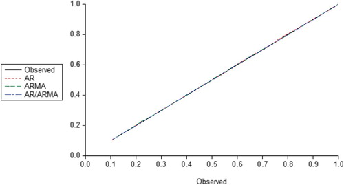
Further comparison was made in terms of the cumulative frequency distribution of the observed and the three models of AR/ARMA, AR and ARMA. Figures 1 and 2 plotted the cumulative frequency distribution of the Observed against each of the three fitted models for Nigerian and US interest rates, respectively. A careful look at Figure 1 in particular shows that the combined AR/ARMA provided the best straight line graph while the other two deviated markedly from the Observed (i.e. the solid line) around 0.4 and 0.9. This is less pronounced for the USA data in Figure 2. From both plots, it is obvious that the AR/ARMA model produces the best straight line graph compared to AR model and ARMA model which clearly shows that the fitted values from the proposed model are closest to the observed than Eni and Mahmud (2008) and Eni (2013), therefore, the best fit to the data points.

Figure 1. A plot of the cumulative frequency distribution of the observed against each of the three fitted models of AR ARMA and AR/ARMA, respectively, for Interest Rate Spread in Nigeria.

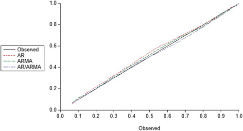
Figure 2. A plot of the cumulative frequency distribution of the observed against each of the three fitted models of AR ARMA and AR/ARMA, respectively, for Interest Rate in USA.

Finally, we conducted a Kolmogorov–Smirnov (K–S) test to confirm our observations from Tables 2 and 3, and Figures 1 and 2. The result is presented in Table 4. In testing the null hypothesis that a model fits the datasets for Nigerian and US interest rates, it is observed that the p-value for the three models were greater than a significant level of $\alpha =0.05,$ which implies that there is no significant evidence against the null. However, we observed further that the proposed had the lowest z-score and consequently, the highest p-value compared to the other two models.² This indicates clearly that the generalisation proposed in this study provides more flexible specification to model time series processes in the presence of errors.

Table 4. K–S test values on observed against various models for Nigeria and USA dataset points.

		AR/ARMA	AR	ARMA
Nigeria	$Z_{K-S}$	0.501	0.504	0.503
	p	0.464	0.458	0.460
USA	$Z_{K-S}$	0.588	0.633	0.653
	p	0.880	0.818	0.787

5. Conclusion

This study formulated a credible, flexible and versatile model capable of accounting for errors from different sources and has been able to apply basic tools such as the autocovariance function, maximum likelihood method, Newton–Raphson iterative method and Kolmogorov–Smirnov test statistic to examine and fit the formulated specification to data. Based on the theoretical results and data application, we concluded that the proposed model is a generalisation of the existing models on AR error and ARMA error.

Empirical results from the application of the proposed model to the Nigerian and US interest rates showed that the error associated with Nigerian interest rates system is essentially a mixture (0.3934, 0.6066) of AR and ARMA and has 0.574 and 0.724 chances of being modelled uniformly as AR and ARMA, respectively. The corresponding probabilities for the US data were (0.6431, 0.3569) for mixture and 0.803 for remaining an AR, and 0.644 for remaining an ARMA. Furthermore, while the Nigerian error system is more likely to switch between AR and ARMA errors with probability 0.426, USA's has lower probability of switching between AR and ARMA with a margin of 0.228 relative to Nigerian system. This indicates that the Nigeria data changes more swiftly from AR to ARMA but less swiftly from ARMA to AR compared to US system. The graphical analysis indicated that the proposed model provided the best fit for the two interest rates datasets considered. This was further confirmed with the Kolmogorov–Smirnov test as the proposed model had more accurate cumulative probabilities, gave the least maximum absolute deviations and consequently the lowest z-scores for the error systems of Nigerian and US interest rates, respectively. Thus, the Nigerian interest rates error pattern more likely follows ARMA than AR, while that of USA has a higher probability of being modelled as AR than ARMA.

Finally, this study discussed AR(1), ARMA(1,1) and the convex combination of ARMA errors. It will certainly enhance research if other versions of time series processes like Autoregressive Conditional Heteroskedasticity (ARCH), Generalised Autoregressive Conditional Heteroskedasticity (GARCH), Seasonal Autoregressive Integrated Moving Average (SARIMA), etc., are considered for volatility and seasonality. More data will be required for better results. Also, properties of the error pattern and the variation with different values of the parameters may be investigated. These may include moments, kurtosis and some other parameters.

Disclosure statement

No potential conflict of interest was reported by the authors.

Additional information

Notes on contributors

S. A. Komolafe

S. A. Komolafe is a student at the Department of Mathematics, Obafemi Awolowo University, Ile-Ife. He obtained M.Sc. in Statistics in Obafemi Awolowo University, Ile-Ife. His area of research includes time series analysis and econometrics.

T. O. Obilade

T. O. Obilade is a Professor of Statistics at the Department of Mathematics, Obafemi Awolowo University in Ile-Ife, Nigeria. He has taught most of the Mathematics and Statistics courses in the department for several decades. Professor Obilade has written many articles. He has also supervised several M.Sc. and Ph.D. theses.

I. O. Ayodeji

I. O. Ayodeji is a Lecturer at the Department of Mathematics, Obafemi Awolowo University, Ile-Ife. She received her Ph.D. in Statistics from Obafemi Awolowo University, Ile- Ife, in 2015. She has to her credit quality articles published in top journals in economics and statistics, including Communications in Statistics – Theory and Methods, African Development Review and the Journal of Applied Mathematics.

A. R. Babalola

A. R. Babalola is an Assistant Lecturer and a Ph.D. student at the Department of Mathematics, Obafemi Awolowo University in Ile-Ife, Nigeria. His research interests include queueing theory and time series analysis.

Notes

1 Readers interested in simulations and estimations of IMA process under the two error patterns of AR and ARMA may kindly refer to Eni and Mahmud (2008) and Eni (2013).

2 One may argue that the p- and z-values of the proposed are just marginally better than the existing models; however, it is known that when sample size is small, as we have in both illustrations, (i.e. for Nigeria, sample size used in Kolmogorov test is 12 while that of US is 16), Kolmogorov test usually masks the extent of deviation between the two distributions under consideration. Tables 2 and 3 of Absolute deviations displayed clear deviations of the existing two models from the Observed compared to the Proposed.

Appendix

Table A1. Cumulative probability frequency of observed $\left(F_0\right(x\left)\right)$ and cumulative probability frequency for fitted models for interest rate data in USA.

	Observed			ARMA/AR			AR			ARMA
Range	Freq.	Cum. Freq.	Cum. Pr., $F_0\left(x\right))$	Freq.	Cum. Freq.	Cum. Pr., $F_1\left(x\right))$	Freq.	Cum. Freq.	Cum. Pr., $F_2\left(x\right))$	Freq.	Cum. Freq.	Cum. Pr., $F_3\left(x\right))$
(0–1]	86	86	0.1067	86	86	0.1067	85	85	0.1055	86	86	0.1067
(1–2]	90	176	0.2184	91	177	0.2196	94	179	0.2221	94	180	0.2233
(2–3]	65	241	0.2990	64	241	0.2990	63	242	0.3002	60	240	0.2978
(3–4]	120	361	0.4479	121	362	0.4491	120	362	0.4491	122	362	0.4491
(4–5]	99	460	0.5707	100	462	0.5732	99	461	0.5720	101	463	0.5744
(5–6]	128	588	0.7295	126	588	0.7295	130	591	0.7333	125	588	0.7295
(6–7]	85	673	0.8349	84	672	0.8337	84	675	0.8375	83	671	0.8325
(7–8]	48	721	0.8945	48	720	0.8933	46	721	0.8945	48	719	0.8921
(8–9]	31	752	0.9330	31	751	0.9318	31	752	0.9330	32	751	0.9318
(9–10]	17	769	0.9541	19	770	0.9553	16	768	0.9529	18	769	0.9541
(10–11]	7	776	0.9628	5	775	0.9651	7	775	0.9615	6	775	0.9615
(11–12]	5	781	0.9690	6	781	0.9690	6	781	0.9690	5	780	0.9677
(12–13]	13	794	0.9851	13	794	0.9851	12	793	0.9839	12	792	0.9826
(13–14]	8	802	0.9950	8	802	0.9950	9	802	0.9950	10	802	0.9950
(14–15]	4	806	1.0000	4	806	1.0000	4	806	1.0000	4	806	1.0000

Table A2. Cumulative probability frequency of observed ($F_0\left(x\right))$ and cumulative probability frequency for fitted models for interest rate spread data in Nigeria.

	Observed			ARMA/AR			AR			ARMA
Range	Freq.	Cum. Freq.	Cum. Pr., $F_0\left(x\right))$	Freq.	Cum. Freq.	Cum. Pr., $F_1\left(x\right))$	Freq.	Cum. Freq.	Cum. Pr., $F_2\left(x\right))$	Freq.	Cum. Freq.	Cum. Pr., $F_3\left(x\right))$
(0–1]	9	9	0.0652	9	9	0.0652	8	8	0.0579	9	9	0.0652
(1–2]	5	14	0.1014	5	14	0.1014	7	15	0.1087	7	16	0.1159
(2–3]	8	22	0.1594	8	22	0.1594	9	24	0.1739	6	22	0.1594
(3–4]	32	54	0.3913	33	55	0.3986	34	58	0.4203	35	57	0.4130
(4–5]	8	62	0.4493	8	63	0.4565	9	67	0.4855	7	64	0.4638
(5–6]	12	74	0.5362	10	73	0.5290	13	80	0.5797	13	77	0.5579
(6–7]	17	91	0.6594	15	88	0.6377	14	94	0.6812	16	93	0.6739
(7–8]	19	110	0.7971	19	107	0.7754	16	110	0.7971	15	108	0.7826
(8–9]	15	125	0.9058	17	124	0.8913	14	124	0.8986	16	124	0.8986
(9–10]	6	131	0.9493	6	130	0.9420	8	132	0.9565	7	131	0.9493
(10–11]	5	136	0.9855	6	136	0.9855	3	135	0.9783	4	135	0.9783
(11–12]	2	138	1.0000	2	138	1.0000	3	138	1.0000	3	138	1.0000

References

- Ayodeji, I. O. (2016). A three-state Markov-modulated switching model for exchange rates. Journal of Applied Mathematics, 2016, 1–9. doi: 10.1155/2016/5061749
- Barnett, V. D. (1967). A note on linear structural relationships with both residual variances are known. Biometrika, 63, 39–50.
- Box, G., & Jenkins, G. (1976). Time series analysis: Forecasting and control. San Francisco, CA: Holden Day.
- Engel, C., & Hamilton, J. (1990). Long swings in the dollar: Are they in the data and do market know it? American Economic Review, 80, 687–713.
- Eni, D. (2013). Parameter estimation of first order IMA model in the presence of ARMA(1,1) errors. Research Journal in Engineering and Applied Sciences, 2(4), 246–50.
- Eni, D., & Mahmud, S. A. (2008). On the parameter estimation of first order IMA model corrupted with AR (1) errors. Global Journal of Pure and Applied Sciences, 14(1), 115–20. doi: 10.4314/gjpas.v14i1.16783
- Eni, D., Ogban, G., Ekpenyong, B., & Atsu, J. (2007). On error handling for a process following AR(1) with MA(1) errors. Journal of Research in Engineering, 4, 102–4.
- Garcia, R., & Perron, P. (1996). An analysis of the real interest rate under regime shifts. The Review of Economics and Statistics, 78, 111–125. doi: 10.2307/2109851
- Kendall, M. G., & Stuart, A. (1961). The advanced theory of statistics. London: Griffin.
- Lindley, D. V. (1947). Regression lines and the linear functional relationship. Supplement to the Journal of the Royal Statistical Society, 9, 218–44. doi: 10.2307/2984115
- Madansky, A. (1959). The fitting of straight lines when both variables are subject to error. Journal of the American Statistical Association, 54, 173–205. doi: 10.1080/01621459.1959.10501505
- Moran, P.A.P. (1971). Estimating structural and functional relationships. Journal of Multivariate Analysis, 1, 232–255. doi: 10.1016/0047-259X(71)90013-3
- Rudelson, M., & Zhou, S. (2017). Errors-in-variables models with dependent measurements. Electronic Journal of Statistics, 11, 1699–1797. doi: 10.1214/17-EJS1234
- Schneeweiss, H., & Shalabh, H. (2007). On the estimation of the linear relation when the error variances are known. Computational Statistics & Data Analysis, 52, 1143–1148. doi: 10.1016/j.csda.2007.06.018
- Yilmazkuday, H., & Akay, K. (2008). An analysis of Turkish economy under regime shifts. Economic Modelling, 25(5), 885–898. doi: 10.1016/j.econmod.2007.11.013