
 ?Mathematical formulae have been encoded as MathML and are displayed in this HTML version using MathJax in order to improve their display. Uncheck the box to turn MathJax off. This feature requires Javascript. Click on a formula to zoom.
Abstract
The mixture cure model is the most popular model used to analyse the major event with a potential cure fraction. But in the real world there may exist a potential risk from other non-curable competing events. In this paper, we study the accelerated failure time model with mixture cure model via kernel-based nonparametric maximum likelihood estimation allowing non-curable competing risk. An EM algorithm is developed to calculate the estimates for both the regression parameters and the unknown error densities, in which a kernel-smoothed conditional profile likelihood is maximised in the M-step, and the resulting estimates are consistent. Its performance is demonstrated through comprehensive simulation studies. Finally, the proposed method is applied to the colorectal clinical trial data.
1. Introduction
In some medical studies, like prostate cancer or breast cancer, it is often observed that a substantial proportion of study patients never experience the event of interest, which are treated as cured or non-susceptible subjects. A number of mixture cure models have been proposed in the literature for analysing such survival data. The two-component mixture cure model can capture cured and uncured patients simultaneously. The early approach of univariate mixture cure model was used to model the survival data by Boag (Citation1949), which assumed that a fraction of the patients are cured from cancer and will never experience the event. Since then, parametric and semiparametric mixture cure models have been proposed (Li & Taylor, Citation2002; Peng & Dear, Citation2000; Peng, Dear, Denham, Citation1998; Sy & Taylor, Citation2000). The proportional hazards (PHMC) model was further discussed by Sy Taylor (Citation2000) and Peng (Citation2003). Besides, Li Taylor (Citation2002), Zhang Peng (Citation2007), Xu Zhang (Citation2009) and Lu (Citation2010) developed the accelerated failure time (AFTMC) model.
Although PHMC model specifies that the effects of the covariates act multipicatively on the hazard function, the AFTMC model regresses the logarithm of the failure time over the covariates, assuming a direct relationship between failure time over the covariates. Li and Taylor (Citation2002) and Zhang and Peng (Citation2007) estimated parameters through EM for the AFTMC model with semiparametric methods, and the large sample properties was discussed in Xu and Zhang (Citation2009). Lu (Citation2010) developed the AFTMC model and the error density was estimated by the kernel method.
The competing risk model is the main tool in explaining more than one event in survival analysis (Crowder, Citation2001; David & Moeschberge, Citation1978; Kalbfleisch & Prentice, Citation2002; Kleinbaum & Klein, Citation2006). There two common approaches for competing risk data, one is the cumulative incidence function (CIF) (Fine & Gray, Citation1999; Kalbfleisch & Prentice, Citation2002; Tai, Machin, White, & Gebski, Citation2001), the other one is cause-specified hazard or subhazard (Fusaro, Bacchetti, & Jewell, Citation1996; Gaynor et al., Citation1993; Klein, Citation2006; Ohneberg & Schumacher, Citation2017; Pintilie, Citation2007). Usually, the marginal hazards equals to the cause-specified hazards when the independence among events of interest are assumed (Gamel, Weller, Wesley, & Feuer, Citation2000; Kuk, Citation1992; Larson & Dinse, Citation1985; Ng & McLachlan, Citation2003). In mixture model, the marginal hazards are the hazards of single risk (Lambert, Thompson, Weston, & Dickman, Citation2006; Yu & Tiwari, Citation2007; Yu, Tiwari, Cronin, & Feuer, Citation2004).
Due to the scarcity of efficient and reliable computational methods, there is little literature dealing with AFTMC model and competing risk data. In this paper, we assume all patients may experience either event 1 or event 2, where event 1 is the primary event with a potential cure rate and event 2 is all other possible events of interest, which are non-curable. Different from the standard competing risk model, there is a cured fraction existed in event 1. For the patients being cured from event 1, they will only experience event 2; while for the patients being uncured from event 1, they will experience either event 1 or event 2. The rest of the paper is organised as follows. In Section 2, the accelerated failure time mixture cure model allowing non-curable competing risk is developed. An EM algorithm is developed to implement the estimation in Section 3, we maximise a kernel-smoothed conditional profile likelihood in the M-step, which is motivated by Zeng and Lin (Citation2007) in efficient estimation for the accelerated failure time model without cure fraction. We show that the estimates are consistent and efficient in the appendix. In addition, the proposed model and method are evaluated by the comprehensive simulation study in Section 4 and illustrated by the real data analysis in Section 5. Conclusions are made in Section 6.
2. Accelerated failure time mixture cure model allowing non-curable competing risk
Consider a study with n subjects. For subject i, let denote the event time undergoing the risk of primary interest and
the event time under other risks. In addition, let
denote the covariates and
the censoring time for subject i.
is used as event indicator (
for event of interest;
for other risk), and define
when
,
,
. The observed data then consist of
.
is the indicator of the uncured patient i subject to the event of primary interest. That is,
means that subject i is subjected to the event of primary interest with uncured probability
. Note that
is not directly observable. As usual, we assume that
is given or independent of
given
.
As commonly done in the mixture cure models, we assume a logistic regression for , i.e.
where
.
To model the competing risk data, we adopt a similar mixture regression approach as studied in Lu and Peng (Citation2008). Note that when ,
. When
, we assume a logistic regression model
Then, we have
and
. Here, we use a logistic link for both
and
, but other link functions, such as the log-log and probit links, can also be used to model
and
.
In addition, we consider a accelerated failure time regression model for given
and
, i.e.
(1)
(1)
(2)
(2) where
is a row vector of unknown parameters,
denotes the error term for the event j with an unknown survival function,
and
are, respectively, the density and survival function of
.
Define the cumulative incidence functions (CIFs) as
(3)
(3) Then, we have
and
Moreover,
(4)
(4) We see that it is just a mixture model with weights
and
on the model of event 1 (primary) and event 2 (others). When only one risk was considered, i.e.
and
, it becomes the simple mixture cure model
.
Define . With known
and
,
, the likelihood function can be written as
(5)
(5) where
. Direct maximisation of the above observed likelihood function is very challenging due to its complex structure. In the next Section, we derive an EM algorithm to maximise the complete likelihood function.
3. EM algorithm
Similar to the standard mixture cure mode, if could be observed, then the complete likelihood function is written as
(6)
(6) It is easy to write the logarithm of the complete likelihood function into four components regarding to their unknown parameters.
where
(7)
(7)
(8)
(8)
(9)
(9)
(10)
(10) and
, here
and
are the hazard function and cumulative functions of
, j=1,2 respectively.
Take as auxiliary variables, and use EM algorithm to find the maximum likelihood estimates of the unknown parameters. The E-step in the EM algorithm computes the conditional expectation of the complete log-likelihood function with respect to three unobserved probabilities
, the probability that uncured patients die from the events of primary interest;
, the probability that uncured patients die from other risks; and
, the probability that cured patients die from other risks, respectively, where m indicates the m-th step in the EM algorithm. These three probabilities sum to 1 and can, respectively, be given by
(11)
(11)
(12)
(12)
(13)
(13)
Let and
, then
. Let
and
and
, then
. The expectations of (Equation7
(7)
(7) ), (Equation8
(8)
(8) ), (Equation9
(9)
(9) ) and (Equation10
(10)
(10) ) can be written as
(14)
(14)
(15)
(15)
(16)
(16)
(17)
(17) The M-step in the EM algorithm is to maximise (Equation14
(14)
(14) ), (Equation15
(15)
(15) ), (Equation16
(16)
(16) ) and (Equation17
(17)
(17) ) with respect to the unknown parameters α, θ,
,
,
and
. Maximising (Equation14
(14)
(14) ) and (Equation15
(15)
(15) ) with respect to α and θ can be easily carried out using the Newton–Raphson algorithm, and maximising
and
in (Equation16
(16)
(16) ) and (Equation17
(17)
(17) )with respect to
,
,
and
can be carried out utilising the approach proposed by Zeng and Lin (Citation2007).
To find a smooth estimator for , or
, for simplify, we take
, or
as example,
and
are similar. We start with the simplest case of a piecewise constant
. To be specific, we partition an interval containing all
into
equally spaced intervals,
, where M denotes an upper bound for the
over all possible
's in a bounded set. A piecewise constant
takes the form
(18)
(18) Then, for any t,
(19)
(19) As
, then (Equation9
(9)
(9) ) can be rewritten as
(20)
(20) By differentiating with respect to
, we see that the solution to the score equation of
is
(21)
(21) After plugging the equations for the
into (Equation20
(20)
(20) ) and discarding the irrelevant component, we obtain the following sieve profile function:
(22)
(22) Note
is not smooth and may have multiple local maxima. Following Zeng and Lin (Citation2007), we further seek a smooth approximation of
by the empirical measure. The kernel smoothed approximation of
is
(23)
(23) where
is the kernel function and
is the bandwidth. The detail of this derivation can be found in the appendix. The selection of the kernel function and bandwidth can be found in Zeng and Lin (Citation2007). We propose to maximise
over
and denote the resulting estimator as
. Because
is a smooth kernel function, we can use the Newton–Raphson algorithm or other gradient-based search algorithms to calculate
. Given
, we estimate
by the following kernel-smoothed estimator:
(24)
(24) The corresponding estimator of
is
(25)
(25) Similar to
and
, the estimator of
and
are
(26)
(26) and
(27)
(27) The M-step in the EM algorithm is to maximise (Equation14
(14)
(14) ), (Equation15
(15)
(15) ), (Equation16
(16)
(16) ) and (Equation17
(17)
(17) ) with respect to the unknown parameters
, which can be easily estimated by the Newton–Raphson method using ‘optim’ function in R.
The EM algorithm is described as follows:
Step 0: Given initial values of ,
,
,
and
.
and
can be estimated by (Equation24
(24)
(24) ) and (Equation26
(26)
(26) ) based on the value of
and
.
Step 1: Update and
by maximising (Equation14
(14)
(14) ) and (Equation15
(15)
(15) ). Update
and
by maxi-mising (Equation23
(23)
(23) ).
Step 2: Update and
via (Equation24
(24)
(24) ) and (Equation26
(26)
(26) ).
Step 3: In the th iteration, calculate
,
,
based on
,
,
,
,
and
from (Equation11
(11)
(11) ), (Equation12
(12)
(12) ), (Equation13
(13)
(13) ).
Step 4: Repeat Steps 1 and 3 until convergence attained. For convergence, we use the criterion, .
The algorithm always converges in our simulation.
4. Simulation
We conducted numerous simulation studies to examine the proposed inference procedures. We generated failure times from the following model:
(28)
(28) where
is standard normal distribution, and
is Bernoulli with 0.5 success probability. We considered three distribution of
: Weibull distribution with different shape parameters, denoted by Weibull
and Weibull
; lognormal distribution with different parameters, denoted by lognormal
and lognormal
; Weibull distribution for the event of interest and lognormal distribution for the other event, which is Weibull
and lognormal
.
for the event of interest for uncured patient and
for other risk event. We assume
in the uncure component
,
for the component in the competing risk
, We generated censoring times from the uniform
distribution, where τ was chosen to produce a
censoring rate. We set n to 100, 500 and 1000.
Following Zeng and Lin (Citation2007), we choose the kernel function to be the standard normal density for convenience and tractability. We used the optimal bandwidths
, where σ is the sample standard deviations of
.
Table reports the biases, mean squared errors (MSE), empirical standard errors (SE), average estimated standard deviations (ESD) with bootstrap sample size 500 and coverage probabilities (CP). From Table , we can see that all biases are relatively small, the SEs and ESDs are close to each other, and the
CPs are close to their nominal levels. With sample size increases, the biases, MSE and SE become smaller.
Table 1. Estimates of parameters for three baseline survivals.
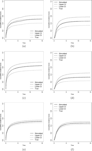
Figures – show the estimates of CIFs of the proposed model along with the true CIFs. We compare the CIFs of the event of primary interest () and other risks (
) with their
pointwise confidence intervals (CI). The estimated CIFs are close to the true values, and it becomes closer as sample sizes increase. All these evidences show that the proposed method performs well, even for small and medium size samples.
Figure 1. Estimated CIFs with Weibull distributions (solid lines), their 95% pointwise confidence intervals (dashed and dotted lines), and the true CIFs (dotdash lines). (a) . (b)
. (c)
. (d)
. (e)
. (f)
.
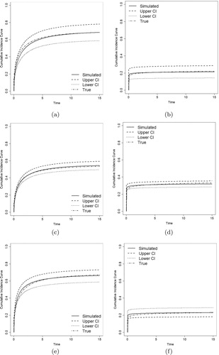
Figure 2. Estimated CIFs with lognormal distributions (solid lines), their 95% pointwise confidence intervals (dashed and dotted lines), and the true CIFs dotdash lines). (a) . (b)
. (c)
. (d)
. (e)
. (f)
.
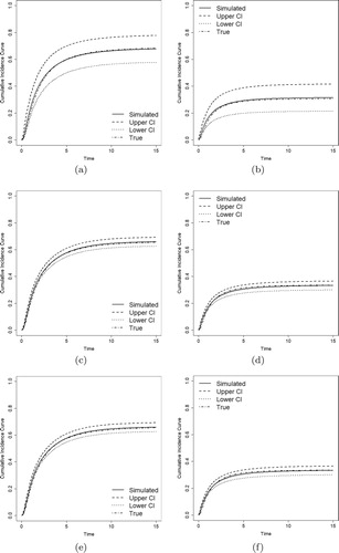
Figure 3. Estimated CIFs with Weibull and lognormal distributions (solid lines), their 95% pointwise confidence intervals (dashed and dotted lines), and the true CIFs (dotdash lines). (a) . (b)
. (c)
. (d)
. (e)
. (f)
.
5. Colorectal cancer clinical trial data
To illustrate the proposed estimation method for the AFT mixture cure model with competing risks data, we consider the colorectal cancer clinical trial data from González et al. (Citation2005), which contains rehospitalisation and death data of patients diagnosed with colorectal cancer between January 1996 and December 1998. The data includes calendar time (in days) of the successive hospitalisations after surgical procedure. Gray test with P=0.0006 provides the evidence for considering the competing risk model in this data set, and González et al. (Citation2005) considered death to be a competing risk to rehospitalisation. However, some patients may never have rehospitalisation after discharge. Thus, we consider time to rehospitalisation as the primary interest and death as other possible event which is non-curable, and analyse the data via the proposed model.
This study included 523 patients. The first hospital readmission time was considered as the day between date of surgery and the first rehospitalisation after discharge related to colorectal cancer. There are patients do not experience both events till the end of study and being treated as the right censoring. We considered drug treatment group (chem=1 for thiotepa drug and 0 for control group) and readmissions for comorbidity (Charlson's index:0, 1–2, 3) for possible risk factors for two events of interest. Thiotepa is a member of the class of alkylating agents, which were among the first anticancer drugs used. Alkylating agents are highly reactive and bind to certain chemical groups found in nucleic acids. These compounds inhibit proper synthesis of DNA and RNA, which leads to apoptosis or cell death. However, since alkylating agents cannot discriminate between cancerous and normal cells, both types of cells will be affected by this therapy. For example, normal cells can become cancerous due to alklyating agents. Thus, thiotepa is a highly cytotoxic compound and can potentially have adverse effects. Consequently, the effects of thiotepa on cancer recurrence and death are not obvious.
For the proposed model, all variables were included in the competing risk event with cured and without cured component. The estimated coefficients and their standard deviations for proposed model are listed in Table . Based on the uncure part and competing risk part, both Charlson's index (0) and Charlson's index(1−2) have significant impact. Similarly, both treatment and Charlson's index(1−2) show significant impact on whether patients will experience the rehospitalisation or death.
Table 2. Results for colorectal cancer clinical trial data.
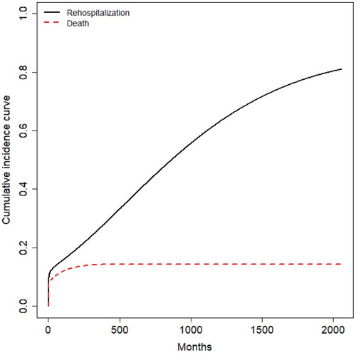
After using the (Equation3(3)
(3) ), we calculated and plotted the cumulative incidence curves for rehospitalisation and death of colorectal cancer in the Figure . Figure shows the competing relationship between the rehospitalisaion and death clearly, and the rehospita-lisaion has a higher rate than death.
Figure 4. Proposed model.
6. Discussions and conclusions
In this paper, we developed a new accelerated failure time mixture cure model allowing non-curable competing risk. Comparing with the existing models, this model can better capture the cure rate of disease than the traditional mixture cure model. The semiparametric estimation based on the EM algorithm can be easily got with the help of existing popular R packages. Although the variance estimation is based on the bootstrap due to the complex structure of model, the comprehensive simulation shows that the performance is reasonable even when the resampling size is small.
Acknowledgements
The research is supported by the Natural Science Foundation of China (Nos. 11271136, 81530086) and the 111 Project of China (No. B14019).
Disclosure statement
No potential conflict of interest was reported by the authors.
Additional information
Notes on contributors
Yijun Wang
Yijun Wang is a PhD candidate in the College of Statistics, East China Normal University, Shanghai, China. Her research interests include Bayesian statistics, reliability statistics and biostatistics.
Jiajia Zhang
Jiajia Zhang is a professor of biostatistics in the Department of Epidemiology and Biostatistics, University of South Carolina, USC. She received her PhD degree from Memorial University. Her professional publications and research interests have focused on survival analysis,semiparametric estimation methods and spatial survival analysis.
Yincai Tang
Yincai Tang is professor of statistics in the College of Statistics, East China Normal University, Shanghai, China. He received his PhD degree from East China Normal University. His professional publications and research interests have focused on lifetime data analysis, degradation data analysis, big data analysis and Bayesian inference.
References
- Boag, J.W. (1949). Maximum likelihood estimates of the proportion of patients cured by cancer therapy. Journal of the Royal Statistical Society. Series B (Methodological), 11(1), 15–53. doi: 10.1111/j.2517-6161.1949.tb00020.x
- Crowder, M. (2001). Classical competing risk. London: Chapman and Hall/CRC.
- David, H., & Moeschberge, M. (1978). The theory of competing risks. London: Griffn.
- Fine, J., & Gray, R. (1999). A proportional hazards model for the subdistribution of a competing risk. Journal of the American Statistical Association, 94(446), 496–509. doi: 10.1080/01621459.1999.10474144
- Fusaro, R., Bacchetti, P., & Jewell, N. (1996). A competing risks analysis of presenting aids diagnoses trends. Biometrics, 52, 211–225. doi: 10.2307/2533157
- Gamel, J., Weller, E., Wesley, M., & Feuer, E. (2000). Parametric cure models of relative and cause-specific survival for grouped survival times. Computer Methods and Programs in Biomedicine, 61(2), 99–110. doi: 10.1016/S0169-2607(99)00022-X
- Gaynor, J., Feuer, E., Tan, C., Wu, D., Little, C., Straus, D., …Brennan, M. (1993). On the use of cause-specific failure and conditional failure probabilities: Examples from clinical oncology data. Journal of the American Statistical Association, 88(422), 400–409. doi: 10.1080/01621459.1993.10476289
- González, J. R., Fernandez, E., Moreno, V., Ribes, J., Peris, M., Navarro, M., …Borrás, J. M. (2005). Sex differences in hospital readmission among colorectal cancer patients. Journal of Epidemiology & Community Health, 59(6), 506–511. doi: 10.1136/jech.2004.028902
- Kalbfleisch, J.D., & Prentice, R.L. (2002). The statistical analysis of failure time data. New York: John Wiley & Sons.
- Klein, J. (2006). Modelling competing risks in cancer studies. Statistics in Medicine, 25(6), 1015–1034. doi: 10.1002/sim.2246
- Kleinbaum, D., & Klein, M. (2006). Survival analysis: A self-learning text. New York: Springer Science & Business Media.
- Kuk, A. (1992). A semiparametric mixture model for the analysis of competing risks data. Australin Jounal of Statistics, 34(2), 169–180.
- Lambert, P., Thompson, J., Weston, C., & Dickman, P. (2006). Estimating and modeling the cure fraction in population-based cancer survival analysis. Biostatistics (Oxford, England), 8(3), 576–594. doi: 10.1093/biostatistics/kxl030
- Larson, M., & Dinse, G. (1985). A mixture model for the regression analysis of competing risks data. Applied Statistics, 34(3), 201–211. doi: 10.2307/2347464
- Li, C., & Taylor, J. (2002). A semi-parametric accelerated failure time cure model. Statistics in Medicine, 21(21), 3235–3247. doi: 10.1002/sim.1260
- Lu, W. (2010). Efficient estimation for an accelerated failure time model with a cure fraction. Statistica Sinica, 20, 661–674.
- Lu, W., & Peng, L. (2008). Semiparametric analysis of mixture regression models with competing risks data. Lifetime Data Analysis, 14(3), 231–252. doi: 10.1007/s10985-007-9077-6
- Ng, S., & McLachlan, G. (2003). An em-based semi-parametric mixture model approach to the regression analysis of competing-risks data. Statistics in Medicine, 22(7), 1097–1111. doi: 10.1002/sim.1371
- Ohneberg, K., Schumacher, M., & Beyersmann, J. (2017). Modelling two cause-specific hazards of competing risks in one cumulative proportional odds model?. Statistics in Medicine, 36(27), 4353–4363. doi: 10.1002/sim.7437
- Peng, Y. (2003). Fitting semiparametric cure models. Computational Statistics & Data Analysis, 41(3), 481–490. doi: 10.1016/S0167-9473(02)00184-6
- Peng, Y., & Dear, K. B. (2000). A nonparametric mixture model for cure rate estimation. Biometrics, 56(1), 237–243. doi: 10.1111/j.0006-341X.2000.00237.x
- Peng, Y., Dear, K. B., & Denham, J. (1998). A generalized f mixture model for cure rate estimation. Statistics in Medicine, 17(8), 813–830. doi: 10.1002/(SICI)1097-0258(19980430)17:8<813::AID-SIM775>3.0.CO;2-#
- Pintilie, M. (2007). Analysing and interpreting competing risk data. Statistics in Medicine, 26(6), 1360–1367. doi: 10.1002/sim.2655
- Sy, J., & Taylor, J. (2000). Estimation in a cox proportional hazards cure model. Biometrics, 56(1), 227–236. doi: 10.1111/j.0006-341X.2000.00227.x
- Tai, B., Machin, D., White, I., & Gebski, V. (2001). Competing risks analysis of patients with osteosarcoma: A comparison of four different approaches. Statistics in Medicine, 20(5), 661–684. doi: 10.1002/sim.711
- Van Der VaartJon, A., & Wellner, J. (1996). Weak convergence and empirical processes. New York, NY: Springer.
- Xu, L., & Zhang, J. (2009). An alternative estimation method for the semiparametric accelerated failure time mixture cure model. Communications in Statistics-Simulation and Computation, 38(9), 1980–1990. doi: 10.1080/03610910903180657
- Yu, B., & Tiwari, R. (2007). Application of em algorithm to mixture cure model for grouped relative survival data. Journal of Data Science, 5, 41–51.
- Yu, B., Tiwari, R., Cronin, K., & Feuer, E. (2004). Cure fraction estimation from the mixture cure models for grouped survival data. Statistics in Medicine, 23, 1733–1747. doi: 10.1002/sim.1774
- Zeng, D., & Lin, D. (2007). Efficient estimation for the accelerated failure time model. Journal of the American Statistical Association, 102(480), 1387–1396. doi: 10.1198/016214507000001085
- Zhang, J., & Peng, Y. (2007). A new estimation method for the semiparametric accelerated failure time mixture cure model. Statistics in Medicine, 26(16), 3157–3171. doi: 10.1002/sim.2748
Appendix
Brief description of approximation for the . When
,
, and
, according to the Donsker theorem, we obtain
Using the multiplier central limit theorem of Van Der VaartJon and Wellner (Citation1996), we have
Since
as
, we can obtain
Uniformly in β and
. Note, for the last term, we have
Then,
Similar to Zeng and Lin (Citation2007), we choose a kernel function
with bandwidth
. The theory of kernel estimation indicates that under suitable regularity conditions,
and
Thus we approximate
by
The Kernel-smoothed approximation of the likelihood function is
Discarding the constant term, we obtain the following log-likelihood function,