Discussion of prior-based Bayesian information criterion (PBIC) by M.J. Bayarria, James O. Berger, Woncheol Jang, Surajit Ray, Luis R. Pericchi, and Ingmar Visser

We congratulate the authors on their innovative and illuminating contribution. Their paper should not only lead to more refined and defensible applications of the Bayesian information criterion (BIC) through their proposed variants, but should also facilitate a deeper understanding of BIC and its theoretical underpinnings.

The development of the prior-based BIC variants, PBIC and PBIC*, results from a reconsideration of the Laplace approximation employed in the large-sample justification for BIC. The authors' more nuanced application of the Laplace approximation leads to the inclusion of terms based on (1) the log of the determinant of the observed information for those parameters that are common to all of the candidate models, (2) standardised estimates of the transformed parameters for those parameters that vary among the candidate models, and (3) an ‘effective sample size’ for each transformed parameter. The terms based on (2) and (3) replace the conventional penalty term of BIC.

An additional refinement to BIC could be incorporated based on terms governed by the prior probabilities assigned to each of the candidate models. To introduce such a correction, we consider the initial stages of the development that leads to BIC.

Assume that the observed $\mathbf{x}$ is to be described using a model ${\mathcal{M}}_k$ selected from a set of candidates ${\mathcal{M}}_1,{\mathcal{M}}_2,\dots ,{\mathcal{M}}_L$. Suppose that each ${\mathcal{M}}_k$ is uniquely parameterised by a vector ${\mathit{\theta }}_k$ $(k\in \{1,2,\dots ,L\left\}\right)$. Let $l\left({\mathit{\theta }}_k|\mathbf{x}\right)$ denote the likelihood for $\mathbf{x}$ based on ${\mathcal{M}}_k$.

Let $p\left({\mathcal{M}}_k\right)$ denote a discrete prior over the models ${\mathcal{M}}_1,{\mathcal{M}}_2,\dots ,{\mathcal{M}}_L$, specified so that $p\left({\mathcal{M}}_k\right)>0$ for all $k\in \{1,2,\dots ,L\}$, and $\sum _{k=1}^{L}p\left({\mathcal{M}}_k\right)=1$. Let $\pi \left({\mathit{\theta }}_k|{\mathcal{M}}_k\right)$ denote a prior on ${\mathit{\theta }}_k$ given the model ${\mathcal{M}}_k$.

Through the application of Bayes' Theorem, for the joint posterior of ${\mathcal{M}}_k$ and ${\mathit{\theta }}_k$, we have $h\left(\right({\mathcal{M}}_k,{\mathit{\theta }}_k\left)|\mathbf{x}\right)\propto p\left({\mathcal{M}}_k\right)\pi \left({\mathit{\theta }}_k|{\mathcal{M}}_k\right)l\left({\mathit{\theta }}_k|\mathbf{x}\right).$

Here, the constant of proportionality, say $K\left(\mathbf{x}\right)$, depends on the data $\mathbf{x}$, yet not on the constructs for model ${\mathcal{M}}_k$.

A Bayesian model selection rule might aim to choose the model ${\mathcal{M}}_k$ which is a posteriori most probable. For the posterior probability for ${\mathcal{M}}_k$, we then have $P\left({\mathcal{M}}_k|\mathbf{x}\right)=K\left(\mathbf{x}\right)p\left({\mathcal{M}}_k\right)\int l\left({\mathit{\theta }}_k|\mathbf{x}\right)\pi \left({\mathit{\theta }}_k|{\mathcal{M}}_k\right)d{\mathit{\theta }}_k.$ If we consider minimising $-2\log P\left({\mathcal{M}}_k|\mathbf{x}\right)$ as opposed to maximising $P\left({\mathcal{M}}_k|\mathbf{x}\right)$, we obtain $\begin{array}{rl}& -2\log P\left({\mathcal{M}}_k|y\right)\\ & =-2\log K\left(\mathbf{x}\right)-2\log p\left({\mathcal{M}}_k\right)\\ & -2\log \left\{\int l\left({\mathit{\theta }}_k|\mathbf{x}\right)\pi \left({\mathit{\theta }}_k|{\mathcal{M}}_k\right)d{\mathit{\theta }}_k\right\}.\end{array}$ Since the term involving $K\left(\mathbf{x}\right)$ does not vary in accordance with the structure of the model ${\mathcal{M}}_k$, for the purpose of model selection, this term can be discarded. We thereby obtain (1) $\begin{array}{r}-2\log p\left({\mathcal{M}}_k\right)-2\log \left\{\int l\left({\mathit{\theta }}_k|\mathbf{x}\right)\pi \left({\mathit{\theta }}_k|{\mathcal{M}}_k\right)d{\mathit{\theta }}_k\right\}.\end{array}$(1) The authors' variants of BIC result through a refined approximation of the integral $\int l\left({\mathit{\theta }}_k|\mathbf{x}\right)\pi \left({\mathit{\theta }}_k|{\mathcal{M}}_k\right)d{\mathit{\theta }}_k.$

In comparing candidate models based on differences in (1(1) $\begin{array}{r}-2\log p\left({\mathcal{M}}_k\right)-2\log \left\{\int l\left({\mathit{\theta }}_k|\mathbf{x}\right)\pi \left({\mathit{\theta }}_k|{\mathcal{M}}_k\right)d{\mathit{\theta }}_k\right\}.\end{array}$(1) ), the terms $-2\log p\left({\mathcal{M}}_k\right)$ are (i) immaterial under a uniform prior distribution $p\left({\mathcal{M}}_k\right)$, and (ii) negligible in large-sample settings where the prior probabilities are not markedly different. In the asymptotic justification of BIC, these terms are discarded. However, the terms involving $p\left({\mathcal{M}}_k\right)$ could play a role in smaller sample settings where candidate models are differentially favoured (e.g. Neath & Cavanaugh, 1997).

Additionally, a uniform prior on the candidate models can lead to inconsistency in high-dimensional sparse settings. To further explore this potential problem, consider a regression setting based on $P$ potential covariates. Let $s$ refer to the number of true ‘active’ regression parameters in the generating model, and let the saturation level $\omega$ refer to the proportion of all $P$ parameters that are in the generating model, so that $\omega =s/P$. The sparsity level (i.e. the proportion of regression parameters that are truly inactive) is simply $(1-\omega )$.

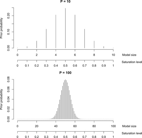
Assuming a uniform prior on the collection of candidate models induces a marginal distribution on the saturation level $\omega$ that becomes increasingly concentrated about $\omega =0.5$ as $P$ increases. For example, consider performing best-subsets selection with $P$ =10 covariates. One might perceive that a defensible approach for determining the final model would be to choose the fitted model corresponding to the lowest BIC. However, since BIC implicitly imposes a uniform prior on the candidate models, and since there are more models with 5 covariates than with 1 or 2 covariates, BIC favours models of size 5 over models of size 1 or 2. In fact, the prior distribution for model size is centred among values near 5; see Figure 1. As $P$ grows, this prior becomes increasingly concentrated around $P$/2. Consequently, the prior distribution on the saturation level becomes progressively more dense around $\omega =0.5$.

Figure 1. The prior instituted by BIC on the marginal distribution of model size (and, consequently, the saturation level) for $P=10$ (top) and $P=100$ (bottom).

Chen and Chen (2008) proffer a solution to this problem: the extended Bayesian information criterion (EBIC). EBIC corrects for the prior imbalance in model size by incorporating an additional term in the formulation of BIC that penalises a model in accordance with the number of candidate models of that size. Let $m_k$ denote the dimension of the regression parameter vector for ${\mathcal{M}}_k$. In the context of best-subsets selection, EBIC is defined as $\begin{array}{rl}\mathrm{EBIC}& =-2\log l\left({\hat{\mathit{\theta }}}_k|\mathbf{x}\right)+m_k\log n+2\gamma \log \left(\genfrac{}{}{0em}{}{P}{m_k}\right)\\ & =\mathrm{BIC}+2\gamma \log \left(\genfrac{}{}{0em}{}{P}{m_k}\right).\end{array}$

The additional penalty term for EBIC can be conveniently conceptualised in the context of the ubiquitous statistical metaphor of balls and urns. In any variable selection problem, each covariate can be viewed as a ball in an urn consisting of $P$ balls. Each model ${\mathcal{M}}_k$ is defined by a random draw, without replacement, of $m_k$ balls from that urn. There are $\left(\genfrac{}{}{0em}{}{P}{m_k}\right)$ ways of selecting the $m_k$ balls, which provides the reason that this combinatorics term arises in the criterion development.

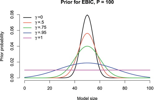
The additional penalty term of EBIC involves a tuning parameter $\gamma$, which is fixed at a value between 0 and 1, inclusive. Different values of $\gamma$ lead to important special cases of the criterion, which are depicted in Figure 2. If $\gamma =0$, EBIC becomes the original BIC. Setting $\gamma =1$ yields a uniform prior on the marginal distribution of model size (and consequently, $\omega$). However, setting $\gamma =1$ leads to a criterion that can be quite conservative in practice. The specification of $\gamma$ is associated with different consistency properties. Broadly speaking, BIC will be inconsistent when $P>\sqrt{n}$, and EBIC corrects for this. Note that since $\gamma \in [0,1]$, the penalty for EBIC will always be greater than or equal to BIC; thus, EBIC will always be at least as conservative as BIC, if not more. A more extensive discussion about the specification of $\gamma$ and related consistency implications can be found in Chen and Chen (2008).

In the best-subsets setting, a similar motivation modifies the prior distributions for all of the models to induce a more formal preference for sparse models (Bogdan, Ghosh, & Doerge, 2004; Bogdan, Ghosh, & Zak-Szatkowska, 2008). The resulting criterion is referred to as the modified Bayesian information criterion (mBIC). Unlike the symmetric priors of BIC and EBIC, the formulation of mBIC utilises a right-skewed prior probability mass function on model size, where the degree of skewness is governed by the saturation level $\omega$. For mBIC, instead of specifying a $\gamma$ parameter, one must specify the ‘expected’ or ‘central’ saturation level, which we will denote as $w$. For a central saturation level $w$, and for a model ${\mathcal{M}}_k$ with $m_k$ parameters, $p\left({\mathcal{M}}_k\right)=w^{m_k}(1-w{)}^{P-m_k}.$ Thus, mBIC views each coefficient as a random draw from an underlying population of effects where $wP$ are active and $(1-w)P$ are inactive, but we do not know which are which a priori.

Figure 2. Marginal distributions for model size resulting from the $\gamma$ parameter for EBIC.

Of course, of the two terms in (1(1) $\begin{array}{r}-2\log p\left({\mathcal{M}}_k\right)-2\log \left\{\int l\left({\mathit{\theta }}_k|\mathbf{x}\right)\pi \left({\mathit{\theta }}_k|{\mathcal{M}}_k\right)d{\mathit{\theta }}_k\right\}.\end{array}$(1) ), the term based on the integral $\int l\left({\mathit{\theta }}_k|\mathbf{x}\right)\pi \left({\mathit{\theta }}_k|{\mathcal{M}}_k\right)d{\mathit{\theta }}_k$ is of primary importance; the authors have justifiably focussed on refining the approximation of this integral in the development of their BIC variants. However, the inclusion of the additional terms $-2\log p\left({\mathcal{M}}_k\right)$ in PBIC and PBIC* could potentially be beneficial in instances where it is justifiable to employ priors $p\left({\mathcal{M}}_k\right)$ that differentially favour certain models in the candidate collection.

Disclosure statement

No potential conflict of interest was reported by the authors.

ORCID

Ryan A. Peterson  http://orcid.org/0000-0002-4650-5798

Joseph E. Cavanaugh  http://orcid.org/0000-0002-0514-7664

Additional information

Notes on contributors

Ryan A. Peterson

Dr Ryan A. Peterson recently received his Ph.D. from the Department of Biostatistics in the College of Public Health at the University of Iowa. In the summer of 2019, he will be joining the faculty of the Department of Biostatistics and Informatics in the Colorado School of Public Health at the University of Colorado Anschutz Medical Campus. His methodological research interests include variable selection, model selection, machine learning, high-dimensional data analysis, and computational statistics.

Joseph E. Cavanaugh

Dr Joseph E. Cavanaugh is a Professor of Biostatistics and Head of the Department of Biostatistics in the College of Public Health at the University of Iowa. He holds a secondary appointment in the Department of Statistics and Actuarial Science and is an affiliate professor in the Applied Mathematical and Computational Sciences interdisciplinary doctoral programme. His methodological research interests include variable selection, model selection, time series analysis, modelling diagnostics, and computational statistics.

References

- Bogdan, M., Ghosh, J. K., & Doerge, R. W. (2004). Modifying the Schwarz Bayesian information criterion to locate multiple interacting quantitative trait loci. Genetics, 167, 989–999. doi: 10.1534/genetics.103.021683
- Bogdan, M., Ghosh, J. K., & Zak-Szatkowska, M. (2008). Selecting explanatory variables with the modified version of the Bayesian information criterion. Quality and Reliability Engineering International, 24, 627–641. doi: 10.1002/qre.936
- Chen, J., & Chen, Z. (2008). Extended Bayesian information criteria for model selection with large model spaces. Biometrika, 95, 759–771. doi: 10.1093/biomet/asn034
- Neath, A. A., & Cavanaugh, J. E. (1997). Regression and time series model selection using variants of the Schwarz information criterion. Communications in Statistics – Theory and Methods, 26, 559–580. doi: 10.1080/03610929708831934