Empirical likelihood estimation in multivariate mixture models with repeated measurements

Abstract

Multivariate mixtures are encountered in situations where the data are repeated or clustered measurements in the presence of heterogeneity among the observations with unknown proportions. In such situations, the main interest may be not only in estimating the component parameters, but also in obtaining reliable estimates of the mixing proportions. In this paper, we propose an empirical likelihood approach combined with a novel dimension reduction procedure for estimating parameters of a two-component multivariate mixture model. The performance of the new method is compared to fully parametric as well as almost nonparametric methods used in the literature.

Keywords:

• Empirical likelihood
• estimating equation
• repeated measurements
• multivariate mixture model

1. Introduction

Mixture models provide a flexible way of modelling complex data obtained from a population with observed or unobserved heterogeneity. Mixture models have been applied in astronomy, biology, fishery, human genetics, and other scientific areas of research. See Titterington, Smith, and Makov (1985), Lindsay (1995), McLachlan and Peel (2000), and references therein.

We consider a special multivariate mixture model where repeated measurements are available for each subject. Let ${\mathit{X}}_1,\dots ,{\mathit{X}}_n$ be independent and identically distributed (i.i.d.) d-variate random vectors from a finite mixture model with m components. If the elements of the vector ${\mathit{X}}_i$ are independent conditional on belonging to a subpopulation, then the mixture density is given by (1) $h\left(\mathit{x}\right)=\sum _{j=1}^m{\pi }_j\prod _{r=1}^d{f}_{jr}\left(x_r\right),$(1) where ${\pi }_j$'s are mixing proportions such that $\sum _{j=1}^m{\pi }_j=1$, ${\pi }_j>0$ for all j, and $f(\cdot )$, with or without subscripts, denotes a univariate density function.

The above data structure is quite common especially in social sciences where measurements are taken repeatedly for various reasons. For example, the goal of research on preschool children's inclusion task responses is to study different solution strategies with which young children solve a given cognitive task. The solution strategy is often called the latent variable since it is hidden and unobservable. A group of preschool children can be considered as a sample from a mixture model where the components correspond to the various solution strategies; see Thomas and Horton (1997). In a simplified setting, one could assume that there are two main solution strategies which lead to a mixture model with two components.

Many researchers studied the nonparametric identifiability of the above multivariate mixture model. Hall and Zhou (2003) showed that the model (1(1) $h\left(\mathit{x}\right)=\sum _{j=1}^m{\pi }_j\prod _{r=1}^d{f}_{jr}\left(x_r\right),$(1) ) is always nonparametrically unidentifiable when d=2 and m=2. Under some mild regularity conditions, Hall and Zhou (2003) proved that the two-component mixture model is nonparametrically identifiable for $d\ge 3$. Kasahara and Shimotsu (2014) discussed the identifiability of the number of components in multivariate mixture models in which each component distribution has independent marginals. Hettmansperger and Thomas (2000) considered the situation where the elements of the vector ${\mathit{X}}_i$ are, not only conditionally independent, but also identically distributed. Under such an assumption, the mixture density (1(1) $h\left(\mathit{x}\right)=\sum _{j=1}^m{\pi }_j\prod _{r=1}^d{f}_{jr}\left(x_r\right),$(1) ) can be rewritten as (2) $h\left(\mathit{x}\right)=\sum _{j=1}^m{\pi }_j\prod _{r=1}^d{f}_j\left(x_r\right).$(2) They proposed an almost nonparametric approach to estimate the mixing proportions. Their key idea is to categorise data into 0 or 1 by setting an optimal cut point and then apply the EM algorithm to estimate the mixing proportion in the resulting binomial mixture models. Cruz-Medina, Hettmansperger, and Thomas (2004) extended the work of Hettmansperger and Thomas (2000) by transforming the observed vector into a count vector which leads to a multinomial mixture model.

To avoid possible loss of efficiency in categorising continuous data into count data, we propose a nonparametric approach to estimate the mixing proportions using empirical likelihood (EL). The EL, which was first introduced by Owen (1988), is a nonparametric method of inference based on a data-driven likelihood ratio function. This nonparametric and likelihood-based approach has become one of the most effective statistical methods. See Owen (2001) for a comprehensive review. As shown in Qin and Lawless (1994), the EL is a prominent efficient tool in estimating parameters by incorporating estimating equations into constrained maximisation of the empirical likelihood function.

We first develop the proposed methodology for the 3-dimensional mixture models, and later on extend it to higher dimensions. For the multivariate mixture model, we propose linking the various moment estimating equations through the EL to provide a more efficient estimation. In the d-dimensional mixture model, there are $2^d-1$ moment estimating equations. When d is large, it is impracticable to search for the optimal solution. We propose a simple and intuitive bootstrap-like modification of the method. First we obtain K sets of three indices chosen randomly and without replacement from $1,2,\dots ,d$, and then multiply the K nonparametric likelihoods pertinent to the chosen indices to obtain the profile empirical likelihood ratio function.

Our simulation results show that, when the parametric model is correctly specified, our EL estimators perform similarly to the parametric estimators. However, when the parametric model is misspecified, the EL estimators perform uniformly better than the parametric estimators and the almost nonparametric estimators.

The paper is organised as follows. The proposed empirical likelihood approach for multivariate mixture model and its theoretical properties are presented in Section 2. The extension to d-dimensional (d>3) mixtures is also presented. Simulation studies and real data analysis are provided in Section 3. Discussions are given in Section 4.

2. Methodology

We first discuss the methodology for the three-variate mixture model, and then extend to multivariate mixtures with higher dimensions.

2.1. Three-variate mixture model

Let $\mathit{X}=(X_1,X_2,X_3{)}^{\mathrm{T}}$ be a 3-dimensional random vector with distribution function $H\left(\mathit{x}\right)$ and joint probability density function (3) $h\left(\mathit{x}\right)=\pi \prod _{i=1}^3{f}_1\left(x_i\right)+(1-\pi )\prod _{i=1}^3{f}_2\left(x_i\right),$(3) where $0\le \pi \le 1$, and the component density functions $f_1$ and $f_2$ are different but unspecified. This model is a special case of model (2(2) $h\left(\mathit{x}\right)=\sum _{j=1}^m{\pi }_j\prod _{r=1}^d{f}_j\left(x_r\right).$(2) ) with m=2 and d=3.

The parameters of interest are the expectations of the random variables and the mixing proportion π. Suppose ${\mu }_0$ and ${\mu }_1$ are the expected values of the two components: ${\mu }_0=\int x{f}_1\left(x\right)\mathrm{d}x,{\mu }_1=\int x{f}_2\left(x\right)\mathrm{d}x,$ and that they satisfy ${\mu }_0<{\mu }_1$. We then have the following moment estimating equations $\begin{array}{rl}\mathbb{E}\left(X_1{X}_2{X}_3\right)& =\pi {\mu }_0^3+(1-\pi ){\mu }_1^3,\\ \mathbb{E}\left(X_1{X}_2\right)& =\mathbb{E}\left(X_1{X}_3\right)=\mathbb{E}\left(X_2{X}_3\right)\\ & =\pi {\mu }_0^2+(1-\pi ){\mu }_1^2,\\ \mathbb{E}\left(X_1\right)& =\mathbb{E}\left(X_2\right)=\mathbb{E}\left(X_3\right)=\pi {\mu }_0+(1-\pi ){\mu }_1.\end{array}$ There are seven estimating equations in total with three unknown parameters $(\pi ,{\mu }_0,{\mu }_1)$.

Let ${\mathit{x}}_i=(x_{i1},x_{i2},x_{i3}{)}^{\mathrm{T}}$, $i=1,\dots ,n$, be i.i.d. observations from the multivariate mixture model (3(3) $h\left(\mathit{x}\right)=\pi \prod _{i=1}^3{f}_1\left(x_i\right)+(1-\pi )\prod _{i=1}^3{f}_2\left(x_i\right),$(3) ), and $p_i=dH\left({\mathit{x}}_i\right)$. According to Owen (1988), the EL function based on the observed data is (4) $\prod _{i=1}^{n}dH\left({\mathit{x}}_i\right)=\prod _{i=1}^n{p}_i.$(4) Let $\mathit{\theta }=(\pi ,{\mu }_0,{\mu }_1{)}^{\mathrm{T}}$. For the distribution $H\left(\mathit{x}\right)$ under study, feasible $p_i$'s satisfy (5) $\sum _{i=1}^n{p}_i=1,p_i\ge 0,\text{and}\sum _{i=1}^n{p}_i\mathit{g}({\mathit{x}}_i,\mathit{\theta })=\mathbf{0},$(5) where (6) $\mathit{g}({\mathit{x}}_i,\mathit{\theta })=\left(g_1\right({\mathit{x}}_i,\mathit{\theta }),{\mathit{g}}_2^{\mathrm{T}}({\mathit{x}}_i,\mathit{\theta }),{\mathit{g}}_3^{\mathrm{T}}({\mathit{x}}_i,\mathit{\theta }){)}^{\mathrm{T}}$(6) with $g_1({\mathit{x}}_i,\mathit{\theta })=x_{i1}{x}_{i2}{x}_{i3}-\pi {\mu }_0^3-(1-\pi ){\mu }_1^3$, $\begin{array}{rl}{\mathit{g}}_2({\mathit{x}}_i,\mathit{\theta })& =\left(\begin{array}{c}{x}_{i1}{x}_{i2}-\pi {\mu }_0^2-(1-\pi ){\mu }_1^2\\ x_{i1}{x}_{i3}-\pi {\mu }_0^2-(1-\pi ){\mu }_1^2\\ x_{i2}{x}_{i3}-\pi {\mu }_0^2-(1-\pi ){\mu }_1^2\end{array}\right)\text{and}\\ {\mathit{g}}_3({\mathit{x}}_i,\mathit{\theta })& =\left(\begin{array}{c}{x}_{i1}-\pi {\mu }_0-(1-\pi ){\mu }_1\\ x_{i2}-\pi {\mu }_0-(1-\pi ){\mu }_1\\ x_{i3}-\pi {\mu }_0-(1-\pi ){\mu }_1\end{array}\right).\end{array}$ Inference on $\mathit{\theta }$ is usually made through their profile likelihood, which is obtained by maximising (4(4) $\prod _{i=1}^{n}dH\left({\mathit{x}}_i\right)=\prod _{i=1}^n{p}_i.$(4) ) with respect to $p_i$'s subject to the constraints in (5(5) $\sum _{i=1}^n{p}_i=1,p_i\ge 0,\text{and}\sum _{i=1}^n{p}_i\mathit{g}({\mathit{x}}_i,\mathit{\theta })=\mathbf{0},$(5) ). Up to a constant not depending on $\mathit{\theta }$, the resulting empirical log-likelihood is $\ell \left(\mathit{\theta }\right)=-\sum _{i=1}^n\log \{1+{\mathit{\lambda }}^{\mathrm{T}}\mathit{g}({\mathit{x}}_i,\mathit{\theta }\left)\right\},$ where $\mathit{\lambda }$ is the Lagrange multiplier determined by $\frac{1}{n}\sum _{i=1}^n\frac{\mathit{g}({\mathit{x}}_i,\mathit{\theta })}{1+{\mathit{\lambda }}^{\mathrm{T}}\mathit{g}({\mathit{x}}_i,\mathit{\theta })}=\mathbf{0}.$ We can show that in a $O\left(n^{-1/3}\right)$ neighbourhood of the true values of $\mathit{\theta }$, $\mathit{\lambda }=\mathit{\lambda }\left(\mathit{\theta }\right)$ is determined uniquely by an implicit function of $\mathit{\theta }$. We denote the maximum empirical likelihood estimators as $\hat{\mathit{\theta }}=(\hat{\pi },{\hat{\mu }}_0,{\hat{\mu }}_1{)}^{\mathrm{T}}$. Their asymptotic properties are given in the following theorem by Qin and Lawless (1994). When $\mathit{\theta }$ takes its true value ${\mathit{\theta }}_0$, we write $\mathit{g}(\mathit{x},{\mathit{\theta }}_0)$ to be $\mathit{g}\left(\mathit{x}\right)$ for short.

Theorem 2.1

Under the regularity conditions specified in Qin and Lawless (1994). As n goes to infinity, $\sqrt{n}(\hat{\mathit{\theta }}-{\mathit{\theta }}_0)\stackrel{d}{⟶}N(0,{\mathit{V}}_1),$ where

${\mathit{V}}_1={\left[\mathbb{E}{\left\{\frac{\mathrm{\partial }\mathit{g}\left(\mathit{X}\right)}{\mathrm{\partial }\mathit{\theta }}\right\}}^{\mathrm{T}}\left\{\mathbb{E}\mathit{g}\right(\mathit{X}\left){\mathit{g}}^{\mathrm{T}}\right(\mathit{X}){\}}^{-1}\mathbb{E}\left\{\frac{\mathrm{\partial }\mathit{g}\left(\mathit{X}\right)}{\mathrm{\partial }\mathit{\theta }}\right\}\right]}^{-1}.$

With $\left(\mathbf{1}\right(X_1\le t),\mathbf{1}(X_2\le t),\mathbf{1}(X_3\le t\left)\right)$ in place of $\mathit{X}$, we can estimate the underlying distribution functions $F_1\left(t\right)$ and $F_2\left(t\right)$. The asymptotic normality of the resulting empirical likelihood estimators can be established in a similar way to Theorem 2.1.

2.2. Multivariate mixtures with higher dimensions

We now extend the methodology discussed in the previous section to the case with d>3. Suppose the d-variate data ${\mathit{w}}_i=(w_{i1},\dots ,w_{id}{)}^{\mathrm{T}},i=1,\dots ,n$, arise from the mixture model with the following mixture density $h\left({\mathit{w}}_i\right)=\pi \prod _{j=1}^d{f}_1\left(w_{ij}\right)+(1-\pi )\prod _{j=1}^d{f}_2\left(w_{ij}\right).$ In principle, we can adopt the same approach as in the case d=3 in order to make inferences about $\mathit{\theta }$. When d is large, however, the number of estimating equations we must deal with is $\left(\begin{array}{c}d\\ d\end{array}\right)+\left(\begin{array}{c}d\\ d-1\end{array}\right)+\cdots +\left(\begin{array}{c}d\\ 1\end{array}\right)=2^d-1,$ which can be extremely large. Consequently, it is impractical to find the optimal solution to embrace that many estimating equations in the empirical likelihood setup.

We now propose a simple and intuitive solution to the high-dimensional problem. Let $M_d=\left(\genfrac{}{}{0ex}{}{d}{3}\right)$, and ${\mathrm{\Omega }}_i$ ($i=1,2,\dots ,M_d$) be all the possible samples of size 3 from $\{1,2,\dots ,d\}$ drawn by simple random sampling without replacement. We randomly select K sets from $\{{\mathrm{\Omega }}_1,\dots ,{\mathrm{\Omega }}_{M_d}\}$ by simple random sampling without replacement. Let ${\mathrm{\Omega }}_k^{\ast }=\{s_{k1},s_{k2},s_{k3}\}$ ($k=1,2,\dots ,K$) be the resulting K index sets, and ${\mathit{u}}_{ki}=(x_{ki},y_{ki},z_{ki}{)}^{\mathrm{T}}$ denote $(w_{i,s_{k1}},w_{i,s_{k2}},w_{i,s_{k3}}{)}^{\mathrm{T}}$. We assume $s_{k1}<s_{k2}<s_{k3}$ for each k, and treat the data with different ${\mathrm{\Omega }}_k^{\ast }$ as independent samples. The profile empirical likelihood ratio function of $\mathit{\theta }$ based on the selected index sets is $\begin{array}{rl}R\left(\mathit{\theta }\right)& =max\left\{\prod _{k=1}^K\prod _{i=1}^n\left(n{p}_{ki}\right)\left|\sum _{i=1}^n{p}_{ki}=1,p_{ki}\ge 0,\right.\right.\\ & \left.\sum _{i=1}^n{p}_{ki}\mathit{g}({\mathit{u}}_{ki},\mathit{\theta })=\mathbf{0},k=1,\dots ,K\right\},\end{array}$ where the function $\mathit{g}$ is defined in (6(6) $\mathit{g}({\mathit{x}}_i,\mathit{\theta })=\left(g_1\right({\mathit{x}}_i,\mathit{\theta }),{\mathit{g}}_2^{\mathrm{T}}({\mathit{x}}_i,\mathit{\theta }),{\mathit{g}}_3^{\mathrm{T}}({\mathit{x}}_i,\mathit{\theta }){)}^{\mathrm{T}}$(6) ).

Applying the method of constrained optimisation, we have $\begin{array}{rl}G& =\sum _{k=1}^K\sum _{i=1}^n\log \left(n{p}_{ki}\right)-n\sum _{k=1}^K\sum _{i=1}^n{p}_{ki}{\mathit{\lambda }}_k^{\mathrm{T}}\mathit{g}({\mathit{u}}_{ki},\mathit{\theta })\\ & +\sum _{k=1}^K{\gamma }_k\left(\sum _{i=1}^n{p}_{ki}-1\right),\end{array}$ where ${\mathit{\lambda }}_k$ and ${\gamma }_k$ are the Lagrange multipliers. Setting the first derivative of G with respect to $p_{ki}$ to zero, we have $\frac{\mathrm{\partial }G}{\mathrm{\partial }{p}_{ki}}=\frac{1}{p_{ki}}-n{\mathit{\lambda }}_k^{\mathrm{T}}\mathit{g}({\mathit{u}}_{ki},\mathit{\theta })+{\gamma }_k=0.$ Multiplying both sides of the above equation by $p_{ki}$ and summing over i give $\sum _{i=1}^n{p}_{ki}\frac{\mathrm{\partial }G}{\mathrm{\partial }{p}_{ki}}=n+{\gamma }_k=0,$ which leads to ${\gamma }_k=-n$. Therefore, the maximum of $\prod _{k=1}^K\prod _{i=1}^n\left(n{p}_{ki}\right)$ is attained at ${\hat{p}}_{ki}=\frac{1}{n}\frac{1}{1+{\mathit{\lambda }}_k^{\mathrm{T}}\mathit{g}({\mathit{u}}_{ki},\mathit{\theta })},k=1,\dots ,K,$ where the Lagrange multipliers ${\mathit{\lambda }}_k={\mathit{\lambda }}_k\left(\mathit{\theta }\right)$'s are the solutions to $\frac{1}{n}\sum _{i=1}^n\frac{\mathit{g}({\mathit{u}}_{ki},\mathit{\theta })}{1+{\mathit{\lambda }}_k^{\mathrm{T}}\mathit{g}({\mathit{u}}_{ki},\mathit{\theta })}=0.$ Putting ${\hat{p}}_{ki}$ back and taking logarithm, we have the profile empirical log-likelihood ratio function of $\mathit{\theta }$, $\ell \left(\mathit{\theta }\right)=\log \left\{R\right(\mathit{\theta }\left)\right\}=-\sum _{k=1}^K\sum _{i=1}^n\log \{1+{\mathit{\lambda }}_k^{\mathrm{T}}\mathit{g}({\mathit{u}}_{ki},\mathit{\theta }\left)\right\}.$ We show that with probability tending to one, there must be a local maximum point in a very small neighbourhood of the true parameter value of $\mathit{\theta }$. Let ${\mathrm{\Omega }}^{\ast }=\{{\mathrm{\Omega }}_1^{\ast },\dots ,{\mathrm{\Omega }}_K^{\ast }\}$.

Lemma 2.1

Let ${\mathit{\theta }}_0=({\pi }_{\ast },{\mu }_{0\ast },{\mu }_{1\ast })$ be the true value of $\mathit{\theta }$. Suppose $\int |x{|}^9\mathrm{d}{F}_0\left(x\right)+\int |x{|}^9\mathrm{d}{F}_1\left(x\right)<\mathrm{\infty },$ ${\pi }_{\ast }\in (0,1)$ and ${\mu }_{0\ast }\ne {\mu }_{1\ast },$ and that $F_0$ and $F_1$ are non-degenerate distributions. Conditioning on ${\mathrm{\Omega }}^{\ast },$ as $n\to \mathrm{\infty },$ $\ell \left(\mathit{\theta }\right)$ attains its maximum value at some point $\hat{\mathit{\theta }}$ with probability 1 in the interior of the ball $\parallel \mathit{\theta }-{\mathit{\theta }}_0\parallel \le n^{-1/3}$. Let $\hat{\mathit{\lambda }}=({\hat{\mathit{\lambda }}}_1^{\mathrm{T}},\dots ,{\hat{\mathit{\lambda }}}_K^{\mathrm{T}}{)}^{\mathrm{T}}$ with ${\hat{\mathit{\lambda }}}_i=\mathit{\lambda }\left(\hat{\mathit{\theta }}\right)$. Consequently, $\hat{\mathit{\theta }}$ and $\hat{\mathit{\lambda }}$ satisfy $\begin{array}{rl}& {\mathit{Q}}_{kn}(\hat{\mathit{\theta }},{\hat{\mathit{\lambda }}}_k)=0\text{for}k=1,\dots ,K,\text{and}\\ & {\mathit{Q}}_{0n}(\hat{\mathit{\theta }},\hat{\mathit{\lambda }})=0,\end{array}$ where $\begin{array}{rl}{\mathit{Q}}_{kn}(\mathit{\theta },\mathit{\lambda })& =\frac{1}{n}\sum _{i=1}^n\frac{\mathit{g}({\mathit{u}}_{ki},\mathit{\theta })}{1+{\mathit{\lambda }}_k^{\mathrm{T}}\mathit{g}({\mathit{u}}_{ki},\mathit{\theta })},\\ {\mathit{Q}}_{0n}(\mathit{\theta },\mathit{\lambda })& =\frac{1}{n}\sum _{k=1}^K\sum _{i=1}^n\frac{1}{1+{\mathit{\lambda }}_k^{\mathrm{T}}\mathit{g}({\mathit{u}}_{ki},\mathit{\theta })}\\ & {\left(\frac{\mathrm{\partial }\mathit{g}({\mathit{u}}_{ki},\mathit{\theta })}{\mathrm{\partial }\mathit{\theta }}\right)}^{\mathrm{T}}{\mathit{\lambda }}_k.\end{array}$

Lemma 2.1 implies that the proposed EL estimator $\hat{\mathit{\theta }}$ is consistent. Based on Lemma 2.1, we further establish the asymptotic normality of $\hat{\mathit{\theta }}$ in the following theorem. This result is an extension of Theorem 1 in Qin and Lawless (1994). It embraces the correlation structure of the selected elements within the random vectors.

Theorem 2.2

Assume the conditions of Lemma 2.1. Let $S_{11}=\mathbb{E}\left\{\mathit{g}\right(\mathit{X}\left){\mathit{g}}^{\mathrm{T}}\right(\mathit{X}\left)\right\},$ $S_{12}=S_{21}^{\mathrm{T}}=-\mathbb{E}\left\{\mathrm{\partial }\mathit{g}\right(\mathit{X}\left)/\mathrm{\partial }{\mathit{\theta }}^{\mathrm{T}}\right\},$ and ${\mathrm{\Sigma }}_{\mathrm{o}\mathrm{f}\mathrm{f}}=\frac{1}{K(K-1)}\sum _{1\le k\ne j\le K}\mathbb{E}\left\{\mathit{g}\right({\mathit{u}}_{k1}\left){\mathit{g}}^{\mathrm{T}}\right({\mathit{u}}_{j1}\left)|{\mathrm{\Omega }}^{\ast }\right\}.$ Conditioning on ${\mathrm{\Omega }}^{\ast },$ as n goes to infinity, $\sqrt{n}(\hat{\mathit{\theta }}-{\mathit{\theta }}_0)$ converges in distribution to $N(0,{\mathit{V}}_2),$ where $\begin{array}{rl}{\mathit{V}}_2& =\frac{1}{K}(S_{21}{S}_{11}^{-1}{S}_{12}{)}^{-1}\\ & +\frac{K-1}{K}\left(S_{21}{S}_{11}^{-1}{S}_{12}{)}^{-1}\right(S_{21}{S}_{11}^{-1})\\ & {\mathrm{\Sigma }}_{\mathrm{o}\mathrm{f}\mathrm{f}}\left(S_{11}^{-1}{S}_{12}\right)(S_{21}{S}_{11}^{-1}{S}_{12}{)}^{-1}.\end{array}$

If there are no common elements in ${\mathrm{\Omega }}_k^{\ast }$ and ${\mathrm{\Omega }}_j^{\ast }$, then $\mathbb{E}\left\{\mathit{g}\right({\mathit{u}}_{k1}\left){\mathit{g}}^{\mathrm{T}}\right({\mathit{u}}_{j1}\left)|{\mathrm{\Omega }}^{\ast }\right\}=0$. Further, if d is quite large, and there are no common elements in any pair of ${\mathrm{\Omega }}_k^{\ast }$ and ${\mathrm{\Omega }}_j^{\ast }$ ($k\ne j$), then ${\mathrm{\Sigma }}_{\mathrm{o}\mathrm{f}\mathrm{f}}=0$, and ${\mathit{V}}_2=(S_{21}{S}_{11}^{-1}{S}_{12}{)}^{-1}/K$. At the other extreme, if ${\mathrm{\Omega }}_k^{\ast }={\mathrm{\Omega }}_1^{\ast }$ for $k=2,\dots ,K$, then ${\mathrm{\Sigma }}_{\mathrm{o}\mathrm{f}\mathrm{f}}=S_{11}$, and ${\mathit{V}}_2=(S_{21}{S}_{11}^{-1}{S}_{12}{)}^{-1}$. Therefore, the second term in ${\mathit{V}}_2$ stands for the efficiency loss due to the fact that some data are used more than once.

3. Simulation studies and data analysis

3.1. Simulation studies

We have carried out simulations to evaluate the finite-sample performance of the proposed empirical likelihood estimators (EL). For comparison, we have also considered two of its competitors: the maximum likelihood estimators (ML) under the multivariate normal mixture model, and the almost nonparametric estimators based on multinomial mixtures (Cruz-Medina et al. (2004); MN for short). Both the ML and MN estimators can be calculated by the EM algorithm.

We generate data from the mixture model (3(3) $h\left(\mathit{x}\right)=\pi \prod _{i=1}^3{f}_1\left(x_i\right)+(1-\pi )\prod _{i=1}^3{f}_2\left(x_i\right),$(3) ). Different specifications of component distributions $f_1$ and $f_2$ are listed below:

1. (Normal mixtures) $f_1$ and $f_2$ are the density functions of $N({\mu }_1,1)$ and $N({\mu }_2,1)$, respectively. Here ${\mu }_1=0$ and ${\mu }_2=1$ or 2.

2. (Non-central t mixtures) $f_1$ and $f_2$ are the density functions of $t(r,a(r\left){\mu }_1\right)$ and $t(r,a(r\left){\mu }_2\right)$, respectively. Here $t(r,a(r\left)\mu \right)$ denotes a t-distribution with r degrees of freedom, non-centrality parameter $a\left(r\right)\mu$, and mean μ, where $a\left(r\right)=\left(2/r\right)\left(\mathrm{\Gamma }\left(r/2\right)/\mathrm{\Gamma }\left(\right(r-1\left)/2\right)\right)$. Here r=4, ${\mu }_1=0$, and ${\mu }_2=1.5$ or 2.

3. (Chi-square mixtures) $f_1$ and $f_2$ are the density functions of ${\chi }_{{\mu }_1}^2$ and ${\chi }_{{\mu }_2}^2$. Here ${\mu }_1=5$ and ${\mu }_2=10$ or 20.

For each setting, we generate 1000 samples with sample size n=400, d=3 or 6, and $\pi =0.2$, 0.5, or 0.8. When d=6, we set K=8 in the proposed EL method. We calculate the biases and standard deviations of the estimators under comparison, and summarise the results in Tables 1–3.

Table 1. Biases (%) and standard deviations (%) (in parentheses) of different estimators based on 1,000 simulations with n=400. Data were generated from the multivariate mixture model with $f_1$ and $f_2$ being $N({\mu }_1,1)$ and $N({\mu }_2,1)$, respectively. Here ${\mu }_1=0$, ${\mu }_2=1$ or 2 and d=3 or 6.

	d=3			d=6
Method	π	${\mu }_1$	${\mu }_2$	π	${\mu }_1$	${\mu }_2$
	$\pi =0.2$, ${\mu }_2=1$
EL	3.34(14.96)	−4.5(33.33)	2.33(11.54)	0.97(6.52)	0.18(14.11)	0.49(4.95)
MN	16.78(19.18)	13.84(40.78)	10.38(16.05)	2.46(9.62)	−20.72(25.32)	5.83(5.96)
ML	2.19(11.32)	−1.33(23.21)	1.45(8.56)	0.24(3.89)	−0.07(8.73)	0.08(3.28)
	$\pi =0.2$, ${\mu }_2=2$
EL	0.29(3.25)	0.61(13.31)	0.27(4.96)	−0.05(2.39)	−0.10(7.34)	−0.06(2.98)
MN	1.74(5.43)	−32.19(28.69)	10.57(7.03)	0.08(2.53)	−46.28(13.04)	10.53(3.53)
ML	0.10(2.46)	0.16(9.20)	0.07(3.75)	0.01(2.09)	0.11(5.00)	0.14(2.42)
	$\pi =0.5$, ${\mu }_2=1$
EL	0.72(13.16)	−1.09(15.10)	2.46(15.25)	−0.2(6.37)	−0.39(6.81)	−0.14(6.89)
MN	0.94(13.75)	−6.76(23.29)	8.86(23.67)	−0.3(5.50)	−13.79(10.83)	13.04(11.17)
ML	−0.2(10.45)	−1.37(11.76)	0.66(11.46)	−0.29(4.35)	−0.28(4.70)	−0.25(4.81 )
	$\pi =0.5$, ${\mu }_2=2$
EL	0.06(3.68)	0.09(6.54)	0.22(6.49)	−0.16(2.87)	0.01(4.06)	−0.28(3.98)
MN	0.00(4.15)	−16.14(16.52)	16.42(16.16)	−0.15(2.78)	−19.97(7.75)	19.64(6.88)
ML	0.00(2.94)	−0.04(4.94)	0.11(4.96)	−0.17(2.63)	−0.10(2.94)	−0.16(3.08)
	$\pi =0.8$, ${\mu }_2=1$
EL	−3.34(15.06)	−2.09(11.78)	4.23(34.49)	−0.97(7.08)	−0.38(5.06)	0.17(14.21)
MN	−17.77(20.32)	−10.54(16.36)	−14.67(41.56)	−2.17(8.89)	−5.83(5.81)	21.41(22.80)
ML	−3.71(13.25)	−2.26(9.88)	−0.95(25.60)	−0.53(3.90)	−0.23(3.28)	−0.37(8.70)
	$\pi =0.8$, ${\mu }_2=2$
EL	−0.37(3.36)	−0.24(5.07)	−0.07(13.19)	0.01(2.36)	−0.12(3.09)	−0.29(7.01)
MN	−1.95(6.22)	−10.16(7.70)	32.08(32.32)	−0.24(4.00)	−10.3(4.17)	45.26(19.93)
ML	−0.25(2.37)	−0.14(3.81)	0.06(8.70)	0.07(2.09)	−0.07(2.42)	0.12(4.61)

Table 2. Biases (%) and standard deviations (%) (in parentheses) of different estimators based on 1,000 simulations with n=400. Data were generated from the multivariate mixture model with $f_1$ and $f_2$ being $t(4,{\mu }_1)$ and $t(4,{\mu }_2/\{\sqrt{2}\mathrm{\Gamma }\left(3/2\right)/\mathrm{\Gamma }\left(2\right)\left\}\right)$, respectively. Here ${\mu }_1=0$, ${\mu }_2=1.5$ or 2 and d=3 or 6.

	d=3			d=6
Method	π	${\mu }_1$	${\mu }_2$	π	${\mu }_1$	${\mu }_2$
	$\pi =0.2$, ${\mu }_2=1.5$
EL	3.45(15.40)	−7.18(50.85)	3.84(21.38)	−0.49(5.90)	−3.91(20.41)	−1.44(7.11)
MN	9.79(15.66)	−14.9(82.18)	51.68(46.55)	1.08(7.48)	−71.86(67.91)	59.47(43.38)
ML	61.85(12.85)	101.00(22.48)	66.01(59.61)	56.13(21.56)	95.17(35.27)	38.41(37.84)
	$\pi =0.2$, ${\mu }_2=2$
EL	1.13(8.87)	−2.98(37.27)	0.92(13.61)	−0.46(3.92)	−2.47(16.23)	−1.53(6.36)
MN	3.42(8.78)	−51.51(87.04)	59.89(60.83)	0.67(5.98)	−92.36(66.26)	79.47(59.61)
ML	58.3(19.12)	128.91(42.01)	77.41(164.19)	17.33(29.78)	41.3(64.06)	21.8(68.62)
	$\pi =0.5$, ${\mu }_2=1.5$
EL	−0.56(12.44)	−3.27(21.17)	1.19(22.59)	−0.93(5.99)	−1.50(9.17)	−1.98(9.76)
MN	−0.42(11.04)	−31.21(48.91)	61.71(65.51)	0.01(4.61)	−42.77(35.48)	85.2(55.73)
ML	30.44(11.70)	53.29(16.19)	21.03(52.65)	15.15(16.04)	29.22(24.27)	8.13(30.20)
	$\pi =0.5$, ${\mu }_2=2$
EL	−0.61(7.80)	−1.46(15.47)	−0.73(19.03)	−0.54(3.86)	−0.72(7.20)	−2.54(8.42)
MN	−0.48(6.31)	−38.24(44.4)	82.58(64.56)	0.13(3.78)	−51.07(40.48)	109.59(71.1)
ML	19.19(17.25)	46.87(32.11)	29.21(95.27)	−0.01(8.46)	5.37(16.65)	−3.63(36.38)
	$\pi =0.8$, ${\mu }_2=1.5$
EL	−3.74(14.02)	−3.58(15.79)	3.55(50.90)	−1.00(5.70)	−0.74(6.35)	−2.41(19.01)
MN	−12.42(16.63)	−22.01(35.80)	41.44(96.03)	−1.57(8.17)	−18.67(29.21)	116.35(94.33)
ML	−1.71(12.38)	13.9(25.24)	−54.54(46.13)	−4.63(7.52)	7.89(7.06)	−49.65(26.15)
	$\pi =0.8$, ${\mu }_2=2$
EL	−1(6.46)	−1.06(9.54)	−1.50(31.48)	−0.49(3.40)	−0.32(4.88)	−4.20(14.72)
MN	−4.73(10.12)	−23.08(33.81)	100.56(104.09)	−0.69(5.67)	−23.85(28.05)	169.97(103.51)
ML	−6.44(9.50)	8.54(10.14)	−66.54(40.47)	−6.77(5.18)	−0.15(30.64)	−49.79(24.33)

Table 3. Biases (%) and standard deviations (%) (in parentheses) of different estimators based on 1,000 simulations with n=400. Data were generated from the multivariate mixture model with $f_1$ and $f_2$ being ${\chi }_{{\mu }_1}^2$ and ${\chi }_{{\mu }_2}^2$, respectively. Here ${\mu }_1=5$, ${\mu }_2=10$ or 20 and d=3 or 6.

	d=3			d=6
Method	π	${\mu }_1$	${\mu }_2$	π	${\mu }_1$	${\mu }_2$
	$\pi =0.2$, ${\mu }_2=10$
EL	1.72(9.81)	−9.58(106.79)	5.19(37.99)	−0.22(4.61)	−6.59(45.73)	−1.33(18.89)
MN	5.15(11.12)	41.52(125.27)	57.42(40.56)	0.53(4.9)	−14.54(52.22)	63.59(23.5)
ML	3.79(12.44)	−3.66(134.41)	13.29(52.78)	−2.27(4.25)	−22.54(57.72)	−10.11(21.07)
	$\pi =0.2$, ${\mu }_2=20$
EL	0.03(3.06)	1.94(92.73)	−1.27(27.15)	−0.17(2.10)	−0.51(25.73)	−1.22(17.57)
MN	0.27(3.41)	−1.38(91.57)	63.70(35.50)	−0.03(3.37)	−10.19(70.36)	75.51(29.02)
ML	−1.28(3.28)	−25.91(56.89)	−17.70(47.12)	−0.48(2.79)	−5.06(34.02)	−5.14(34.02)
	$\pi =0.5$, ${\mu }_2=10$
EL	−0.24(7.99)	−2.89(38.92)	1.2(48.92)	−0.51(4.19)	−2.26(18.18)	−3.29(24.06)
MN	−0.54(7.31)	7.22(60.73)	71.58(71.78)	0.02(3.33)	0.78(27.14)	96.32(37.29)
ML	−10.06(8.06)	−56.55(59.13)	−48.5(43.21)	−8.14(9.39)	−36.58(59.29)	−45.44(46.36)
	$\pi =0.5$, ${\mu }_2=20$
EL	0.08(2.82)	1.01(51.90)	−1.55(34.49)	−0.04(2.58)	−1.07(11.77)	−2.41(22.25)
MN	0.04(3.66)	2.25(68.84)	96.59(83.74)	−0.01(2.49)	−4.98(28.04)	125.48(47.09)
ML	−1.70(4.21)	−16.59(31.39)	−36.1(59.26)	−1.12(7.03)	−8.23(44.42)	−18.47(101.29)
	$\pi =0.8$, ${\mu }_2=10$
EL	−0.73(6.76)	−1.61(22.24)	2.94(85.03)	−0.38(3.52)	−0.95(11.57)	−7.90(41.22)
MN	−5.67(11.64)	9.08(34.32)	71.59(142.80)	−0.30(3.78)	20.31(14.44)	164.10(73.63)
ML	−20.50(8.55)	−67.61(37.71)	−153.48(48.88)	−15.45(14.64)	−43.67(59.79)	−138.41(67.07)
	$\pi =0.8$, ${\mu }_2=20$
EL	−0.14(2.16)	0.03(12.65)	−2.88(54.59)	−0.06(2.09)	0.00(8.44)	−7.86(37.19)
MN	−0.83(5.43)	1.64(24.09)	245.75(176.53)	−0.22(3.77)	2.40(15.46)	315.56(133.24)
ML	−2.40(2.19)	−13.19(11.43)	−106.07(66.16)	−2.47(13.03)	−10.13(53.34)	−48.96(194.17)

Let us first examine Table 1, where the multivariate normal mixture model is correctly specified. As expected, the ML estimators have the smallest standard deviations in all cases and the smallest absolute biases in most cases. The proposed EL estimators perform very similarly to the ML estimators and both of them are uniformly better than the MN estimators. As ${\mu }_2$ goes further away from ${\mu }_1=0$, all estimators have decreasing standard deviations. This may be because the two component distributions in the mixture model also get further away from each other. When π increases from 0.2 to 0.8, the performances of all the three estimators for ${\mu }_1$ are getting better, while those for ${\mu }_2$ are getting worse. This is probably because as π increases, the multivariate normal mixture contains increasing information about ${\mu }_1$ but decreasing information about ${\mu }_2$. All the three estimators for π have better performance when π lies in the middle than on the boundaries of its parameter space.

However, when data are generated from non-normal mixtures, the ML estimators lose their optimality. From Tables 2–3, we can see that compared with the MN estimators, they have smaller absolute biases in some cases, but larger standard deviations in other cases. The proposed EL estimators perform reasonably well as they have uniformly smaller biases and standard deviations than the other two competitors.

If the mixing proportion is of primary interest, we see that when the multivariate normal mixture is correctly specified, the ML estimator again performs the best and the EL estimator has almost the same reasonable performance. Both of them perform better than the MN estimator. When the model is misspecified, the EL estimator has the best performance followed by the MN estimator. These two estimators usually win the ML estimator by a large amount. For example, in Table 2, when $\pi =0.5$, ${\mu }_2=1.5$, and d=3, all three estimators for π have similar standard deviations, however, the ML estimator has a much larger absolute bias (0.3044) compared with the EL estimator (0.0056), and the MN estimator (0.0042).

When the data dimension d increases from 3 to 6, the standard deviations of both the EL and MN estimators are getting smaller but they have different performances in bias. The absolute biases of the EL estimators are always getting smaller, while those of the ML and MN estimators are not the case. For example, in Table 3, when $\pi =0.2$ and ${\mu }_2=10$, the absolute bias of the MN estimator for ${\mu }_2$ increases from 0.5742 to 0.6359 and that of the ML estimator for ${\mu }_1$ increases from 0.0366 to 0.2254. By contrast, that of the EL estimators for both $({\mu }_1,{\mu }_2)$ decreases from $(0.0958,0.0519)$ to $(0.0659,0.0133)$.

Overall, the EL method exhibits more robust performance than the MN and ML methods for different model specifications. When the normal mixture is correctly specified, the proposed EL estimators have comparable performance as the ML estimators. When the normal mixture is misspecified, the EL estimators perform uniformly better than the other two competitors.

3.2. Data analysis

Reaction time (RT) task is one of the most common experimental methods in psychology to study individual differences. In this section, we apply our proposed empirical likelihood method to a RT data set which was analysed by Cruz-Medina et al. (2004). In this experiment, 197 nine-year-old children were tested on mental rotation task in which a target figure was presented on the left and another one on the right. Children thus had to determine whether the second figure was identical to the first or simply a mirror image instead. The RT was recorded in milliseconds. There were 6 trials, and we considered these trials as d=6 repeated measurements. The time delays between trials were randomly chosen so that children would unable to anticipate the length of delays. The subsequent trials were then expected or assumed to be independent. We display only the histogram of the first measurement of the data in Figure 1; those for the rest are similar. Cruz-Medina et al. (2004) suggested using a two-component mixture to fit the heterogeneous RT distribution.

Since recorded in milliseconds, the RT values range from around 700 to 7000. For convenience, we re-scale them in seconds; the resulting numbers are no greater than 10. Although the mixing proportion π is of primary interest, we calculate the EL, MN and ML estimators for all the three parameters $\pi ,{\mu }_1$ and ${\mu }_2$. The results are tabulated in Table 4. Based on these point estimates, we also provide 95% Wald interval estimates for all the three parameters with variances estimated by 200 bootstrap repetitions.

Figure 1. Histogram of the first measurement of the RT data.

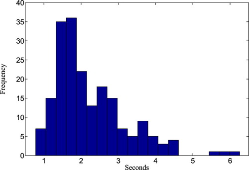
Table 4. Point and interval estimates of the EL, MN and ML methods for $\pi ,{\mu }_1$ and ${\mu }_2$. EL${}_0$: EL with $K=\left(\genfrac{}{}{0ex}{}{6}{3}\right)=20$; EL${}_1$, EL${}_2$, EL${}_3$: EL with K=8; MN${}_1$: MN with cut points $c_1,\dots ,c_{10}$ being the deciles of the empirical distribution, which was suggested by Cruz-Medina et al. (2004) for general use; MN${}_2$: MN with cut points $(c_1,\dots ,c_{10})=(0.5,1,1.2,1.4,1.6,2,2.5,3,4,5)$, which was used by Cruz-Medina et al. (2004) when they analysed this dataset.

Parameter	EL${}_0$	EL${}_1$	EL${}_2$	EL${}_3$	MN${}_1$	MN${}_2$	ML
	Point estimates
π	0.70	0.72	0.68	0.70	0.52	0.59	0.60
${\mu }_1$	1.68	1.70	1.66	1.67	1.58	1.64	1.64
${\mu }_2$	2.90	2.95	2.87	2.91	2.79	2.67	2.64
	95% Interval estimates
π	[0.58, 0.82]	[0.59, 0.84]	[0.55, 0.82]	[0.57, 0.83]	[0.34, 0.70]	[0.39, 0.78]	[0.42, 0.77]
${\mu }_1$	[1.57, 1.79]	[1.59, 1.82]	[1.53, 1.79]	[1.56, 1.79]	[1.39, 1.76]	[1.47, 1.81]	[1.49, 1.78]
${\mu }_2$	[2.58, 3.22]	[2.61, 3.28]	[2.53, 3.22]	[2.57, 3.25]	[2.46, 3.13]	[2.35, 2.98]	[2.35, 2.94]

As mentioned in Section 2.2, the EL estimator depends on the K randomly selected sets ${\mathrm{\Omega }}_k^{\ast }$ ($k=1,2,\dots ,K$). Therefore, we shall obtain different EL estimates in general when applying the EL method more than one time if $K<\left(\genfrac{}{}{0ex}{}{d}{3}\right)$. We apply the EL method with K=8 three times, and denote the results by EL${}_1$, EL${}_2$ and EL${}_3$, respectively. In this example, d=6. When $K=\left(\genfrac{}{}{0ex}{}{6}{3}\right)=20$, the results are denoted by EL${}_0$. We see that the EL estimates with K=8 are very close to those with K=20. This confirms that the proposed random selection strategy works very well. The EL proportion estimates are all around 0.7, and the EL estimates for ${\mu }_1$ and ${\mu }_2$ are around 1.6 and 2.9, respectively.

When applying the MN method, we need to determine the cut points $c_i$'s. For general use, Cruz-Medina et al. (2004) suggested using 10 cut points and choosing $c_1,\dots ,c_{10}$ to be the deciles of the empirical distribution of the data. The resulting MN method, denoted by MN${}_1$, is also the MN method compared in our simulation study. When analysing the RT data, Cruz-Medina et al. (2004) used $(c_1,\dots ,c_{10})=(0.5,1,1.2,1.4,1.6,2,2.5,3,4,5)$. We denote the resulting MN method by MN${}_2$. It seems that the MN results depend to some extent on the choice of cutting points, because the MN${}_1$ proportion estimate 0.52 is quite different from that of MN${}_2$ 0.59. In the meantime, the MN${}_2$ point and interval estimates are both nearly equal to those of the ML method.

According to our simulation studies, the EL method exhibits more robust performance than the MN and ML methods. This indicates that the EL analysis results are more trustworthy than those of the other two methods.

4. Discussions

In this paper, we proposed an empirical likelihood-based estimation method for the parameters of a multivariate two-component mixture model. We discussed three-variate mixtures in detail and extended the methodology to high-dimensional mixtures by giving a permutation-like method which reduces the high-dimensional problem to a three-dimensional situation. The performance and efficiency of the method are demonstrated through a real data example as well as simulation studies. The simulation results show that the proposed method is quite efficient in comparison to both completely parametric and almost nonparametric methods in the literature. Furthermore, the proposed method can accommodate parameter estimation in high-dimensional mixtures by requiring estimation only in three dimensions.

The extension of our approach to mixtures with more than two components is valuable and interesting. Similar to the two-component mixture situation, one can use a set of moment conditions implied by the mixture model to identify and estimate mixing proportions and other component parameters. When the number of components grows, the number of unknown parameters increases. The improvement in the performance of the proposed approach in terms of better identification and higher efficiency may crucially depend on the choice of the set of moment conditions. We will consider it in future research.

Acknowledgements

The authors would like to thank the editor, the AE, and the referee for their insightful comments and suggestions. The authors would like to thank Dr Jing Qin for valuable discussions and many helpful comments.

Disclosure statement

No potential conflict of interest was reported by the authors.

Additional information

Funding

The research is partially supported by the Natural Sciences and Engineering Research Council of Canada (NSERC) Discovery Grants (RGPIN-2018-05846, RGPIN-2018-05981), the National Natural Science Foundation of China (Grant Numbers 11771144, 11501354 and 11501208), and the Chinese 111 Project (B14019).

Notes on contributors

Yuejiao Fu

Yuejiao Fu is an Associate Professor of Statistics in the Department of Mathematics and Statistics at York University, Canada. She received her PhD in Statistics in 2004 from the University of Waterloo. Her research interests include mixture models, empirical likelihood, and statistical genetics.

Yukun Liu

Yukun Liu is a Professor in the School of Statistics, Faculty of Economic and Management, East China Normal University, China. He received his PhD in Statistics in 2009 from Nankai University, China. His research interests include nonparametric and semiparametric statistics based on empirical likelihood and their applications in case-control data, capture-recapture data, selection biased data, and finite mixture models.

Hsiao-Hsuan Wang

Hsiao-Hsuan Wang received her PhD in Statistics in 2010 from York University, Canada. She is now a director in Model Quantification, Enterprise Risk Management, CIBC, Canada.

Xiaogang Wang

Xiaogang Wang is a Professor in Statistics in the Department of Mathematics and Statistics of York University. He is also holding an adjunct position as a senior research fellow at the Institute of Data Science of Tsinghua University in Beijing. He received his PhD in Statistics from the University of British Columbia in 2001. His current research is on statistical analysis of complex data in health and life sciences.

Appendix

Since both Lemma 2.1 and Theorem 2.2 are established conditionally on the K selected sets ${\mathrm{\Omega }}_k^{\ast }$ ($k=1,2,\dots ,K$), for convenience we regard the K selected sets as fixed sets throughout the proofs. Note that ${\mathit{u}}_{ki}$'s are i.i.d. random vectors for fixed k and varying i, while they are not independent for fixed i and varying k.

Proof

Proof of Lemma 2.1

We consider $\mathit{\theta }\in \{\mathit{\theta }|\parallel \mathit{\theta }-{\mathit{\theta }}_0\parallel =n^{-1/3}\}$, which can be rewritten as $\mathit{\theta }={\mathit{\theta }}_0+n^{-1/3}\mathit{v}$ with $\parallel \mathit{v}\parallel =1$. From Qin and Lawless (1994), we can show that $\parallel {\mathit{\lambda }}_k\parallel =O\left(n^{-1/3}\right)$ and $\begin{array}{rl}{\mathit{\lambda }}_k\left(\mathit{\theta }\right)& ={\left\{\frac{1}{n}\sum _{i=1}^n\mathit{g}({\mathit{u}}_{ki},\mathit{\theta }){\mathit{g}}^{\mathrm{T}}({\mathit{u}}_{ki},\mathit{\theta })\right\}}^{-1}\left\{\frac{1}{n}\sum _{i=1}^n\mathit{g}({\mathit{u}}_{ki},\mathit{\theta })\right\}\\ & +o\left(n^{-1/3}\right)\text{(a.s.)}\end{array}$ uniformly about $\mathit{\theta }\in \{\mathit{\theta }|\parallel \mathit{\theta }-{\mathit{\theta }}_0\parallel \le n^{-1/3}\}$, for each $k=1,\dots ,K$. By Taylor's expansion, we have

$\begin{array}{rl}-\ell \left(\mathit{\theta }\right)& =\sum _{k=1}^K\sum _{i=1}^n\log \{1+{\mathit{\lambda }}^{\mathrm{T}}\mathit{g}({\mathit{u}}_{ki},\mathit{\theta }\left)\right\}\\ & =\frac{n}{2}\sum _{k=1}^K{\left[\frac{1}{n}\sum _{i=1}^n\mathit{g}({\mathit{u}}_{ki},\mathit{\theta })\right]}^{\mathrm{T}}{\left[\frac{1}{n}\sum _{i=1}^n\mathit{g}({\mathit{u}}_{ki},\mathit{\theta }){\mathit{g}}^{\mathrm{T}}({\mathit{u}}_{ki},\mathit{\theta })\right]}^{-1}\\ & \times \left[\frac{1}{n}\sum _{i=1}^n\mathit{g}({\mathit{u}}_{ki},\mathit{\theta })\right]+o\left(n^{1/3}\right)\text{(a.s.)}\\ & =\frac{n}{2}\sum _{k=1}^K{\left[\frac{1}{n}\sum _{i=1}^n\mathit{g}({\mathit{u}}_{ki},{\mathit{\theta }}_0)+\frac{1}{n}\sum _{i=1}^n\frac{\mathrm{\partial }\mathit{g}({\mathit{u}}_{ki},{\mathit{\theta }}_0)}{\mathrm{\partial }\mathit{\theta }}\mathit{v}{n}^{-1/3}\right]}^{\mathrm{T}}\\ & \times {\left[\frac{1}{n}\sum _{i=1}^n\mathit{g}({\mathit{u}}_{ki},\mathit{\theta }){\mathit{g}}^{\mathrm{T}}({\mathit{u}}_{ki},\mathit{\theta })\right]}^{-1}\\ & \times \left[\frac{1}{n}\sum _{i=1}^n\mathit{g}({\mathit{u}}_{ki},{\mathit{\theta }}_0)+\frac{1}{n}\sum _{i=1}^n\frac{\mathrm{\partial }\mathit{g}({\mathit{u}}_{ki},{\mathit{\theta }}_0)}{\mathrm{\partial }\mathit{\theta }}\mathit{v}{n}^{-1/3}\right]\\ & +o\left(n^{1/3}\right)\text{(a.s.)}\\ & =\frac{nK}{2}{\left[O\left(n^{-1/2}\right(\log \log n{)}^{1/2})+\mathbb{E}\left(\frac{\mathrm{\partial }\mathit{g}(\mathit{u},{\mathit{\theta }}_0)}{\mathrm{\partial }\mathit{\theta }}\right)\mathit{v}{n}^{-1/3}\right]}^{\mathrm{T}}\\ & \times {\left[\mathbb{E}\left(\mathit{g}\right(\mathit{u},{\mathit{\theta }}_0\left){\mathit{g}}^{\mathrm{T}}\right(\mathit{u},{\mathit{\theta }}_0\left)\right)\right]}^{-1}\\ & \times \left[O\left(n^{-1/2}\right(\log \log n{)}^{1/2})+\mathbb{E}\left(\frac{\mathrm{\partial }\mathit{g}(\mathit{u},{\mathit{\theta }}_0)}{\mathrm{\partial }\mathit{\theta }}\right)\mathit{v}{n}^{-1/3}\right]\\ & +o\left(n^{1/3}\right)\text{(a.s.)}\\ & \ge \left(c/2\right)n^{1/3},\left(\text{a.s.}\right),\end{array}$where c is the smallest eigenvalue of $\mathbb{E}{\left(\frac{\mathrm{\partial }\mathit{g}(\mathit{u},{\mathit{\theta }}_0)}{\mathrm{\partial }\mathit{\theta }}\right)}^{\mathrm{T}}{\left[\mathbb{E}\left(\mathit{g}\right(\mathit{u},{\mathit{\theta }}_0\left){\mathit{g}}^{\mathrm{T}}\right(\mathit{u},{\mathit{\theta }}_0\left)\right)\right]}^{-1}\mathbb{E}\left(\frac{\mathrm{\partial }\mathit{g}(\mathit{u},{\mathit{\theta }}_0)}{\mathrm{\partial }\mathit{\theta }}\right).$ Similarly, $\begin{array}{rl}-\ell \left({\mathit{\theta }}_0\right)& =\frac{n}{2}\sum _{k=1}^K{\left[\frac{1}{n}\sum _{i=1}^n\mathit{g}({\mathit{u}}_{ki},{\mathit{\theta }}_0)\right]}^{\mathrm{T}}\\ & \times {\left[\frac{1}{n}\sum _{i=1}^n\mathit{g}({\mathit{u}}_{ki},{\mathit{\theta }}_0){\mathit{g}}^{\mathrm{T}}({\mathit{u}}_{ki},{\mathit{\theta }}_0)\right]}^{-1}\\ & \times \left[\frac{1}{n}\sum _{i=1}^n\mathit{g}({\mathit{u}}_{ki},{\mathit{\theta }}_0)\right]+o\left(1\right)\text{(a.s.)}\\ & =O(\log \log n).\text{(a.s.)}\end{array}$ Since $\ell \left(\mathit{\theta }\right)$ is a continuous function of $\mathit{\theta }$ when $\mathit{\theta }$ belongs to the ball $\parallel \mathit{\theta }-{\mathit{\theta }}_0\parallel \le n^{-1/3}$, as n is large, $\ell \left(\mathit{\theta }\right)$ must have a maximum point $\hat{\mathit{\theta }}$ in the interior of this ball such that

$\begin{array}{rl}& {\left.\frac{\mathrm{\partial }\ell \left(\mathit{\theta }\right)}{\mathrm{\partial }\mathit{\theta }}\right|}_{\mathit{\theta }=\hat{\mathit{\theta }}}\\ & =-\sum _{k=1}^K\sum _{i=1}^n{\left.\frac{\left(\mathrm{\partial }{\mathit{\lambda }}_k^{\mathrm{T}}\right(\mathit{\theta }\left)/\mathrm{\partial }\mathit{\theta }\right)\mathit{g}({\mathit{u}}_{ki},\mathit{\theta })+\left(\mathrm{\partial }\mathit{g}\right({\mathit{u}}_{ki},\mathit{\theta }\left)/\mathrm{\partial }\mathit{\theta }{)}^{\mathrm{T}}{\mathit{\lambda }}_k\right(\mathit{\theta })}{1+{\mathit{\lambda }}_k^{\mathrm{T}}\left(\mathit{\theta }\right)\mathit{g}({\mathit{u}}_{ki},\mathit{\theta })}\right|}_{\mathit{\theta }=\hat{\mathit{\theta }}}\\ & =-\sum _{k=1}^K\sum _{i=1}^n{\left.\frac{1}{1+{\mathit{\lambda }}_k^{\mathrm{T}}\left(\mathit{\theta }\right)\mathit{g}({\mathit{u}}_{ki},\mathit{\theta })}{\left(\frac{\mathrm{\partial }\mathit{g}({\mathit{u}}_{ki},\mathit{\theta })}{\mathrm{\partial }\mathit{\theta }}\right)}^{\mathrm{T}}{\mathit{\lambda }}_k\left(\mathit{\theta }\right)\right|}_{\mathit{\theta }=\hat{\mathit{\theta }}}\\ & =\mathbf{0}.\end{array}$

Proof

Proof of Theorem 2.2

Taking derivatives about $\mathit{\theta }$ and ${\mathit{\lambda }}^{\mathrm{T}}$, we have $\begin{array}{rl}\frac{\mathrm{\partial }{\mathit{Q}}_{kn}(\mathit{\theta },\mathbf{0})}{\mathrm{\partial }\mathit{\theta }}& =\frac{1}{n}\sum _{i=1}^n\frac{\mathrm{\partial }\mathit{g}({\mathit{u}}_{ki},\mathit{\theta })}{\mathrm{\partial }\mathit{\theta }},\frac{\mathrm{\partial }{\mathit{Q}}_{kn}(\mathit{\theta },\mathbf{0})}{\mathrm{\partial }{\mathit{\lambda }}_j^{\mathrm{T}}}\\ & =-\frac{1}{n}\sum _{i=1}^n\mathit{g}({\mathit{u}}_{ki},\mathit{\theta }){\mathit{g}}^{\mathrm{T}}({\mathit{u}}_{ji},\mathit{\theta }){\delta }_{kj},\\ \frac{\mathrm{\partial }{\mathit{Q}}_{0n}(\mathit{\theta },\mathbf{0})}{\mathrm{\partial }\mathit{\theta }}& =0,\frac{\mathrm{\partial }{\mathit{Q}}_{0n}(\mathit{\theta },\mathbf{0})}{\mathrm{\partial }{\mathit{\lambda }}_k^{\mathrm{T}}}=\frac{1}{n}\sum _{i=1}^n{\left(\frac{\mathrm{\partial }\mathit{g}({\mathit{u}}_{ki},\mathit{\theta })}{\mathrm{\partial }\mathit{\theta }}\right)}^{\mathrm{T}},\end{array}$

for $k,j=1,\dots ,K$, and ${\delta }_{kj}$ is the Kronecker delta. Expanding ${\mathit{Q}}_{kn}(\hat{\mathit{\theta }},\hat{\mathit{\lambda }})$ and ${\mathit{Q}}_{0n}(\hat{\mathit{\theta }},\hat{\mathit{\lambda }})$ at $({\mathit{\theta }}_0,\mathbf{0})$, we have $\begin{array}{rl}\mathbf{0}& ={\mathit{Q}}_{kn}(\hat{\mathit{\theta }},{\hat{\mathit{\lambda }}}_k)={\mathit{Q}}_{kn}({\mathit{\theta }}_0,\mathbf{0})+\frac{\mathrm{\partial }{\mathit{Q}}_{kn}({\mathit{\theta }}_0,\mathbf{0})}{\mathrm{\partial }{\mathit{\lambda }}_k^{\mathrm{T}}}({\hat{\mathit{\lambda }}}_k-\mathbf{0})\\ & +\frac{\mathrm{\partial }{\mathit{Q}}_{kn}({\mathit{\theta }}_0,\mathbf{0})}{\mathrm{\partial }\mathit{\theta }}(\hat{\mathit{\theta }}-{\mathit{\theta }}_0)+o_p\left({\delta }_n\right),\\ \mathbf{0}& ={\mathit{Q}}_{0n}(\hat{\mathit{\theta }},\hat{\mathit{\lambda }})={\mathit{Q}}_{0n}({\mathit{\theta }}_0,\mathbf{0})+\sum _{k=1}^K\frac{\mathrm{\partial }{\mathit{Q}}_{0n}({\mathit{\theta }}_0,\mathbf{0})}{\mathrm{\partial }{\mathit{\lambda }}_k^{\mathrm{T}}}({\hat{\mathit{\lambda }}}_k-\mathbf{0})\\ & +\frac{\mathrm{\partial }{\mathit{Q}}_{0n}({\mathit{\theta }}_0,\mathbf{0})}{\mathrm{\partial }\mathit{\theta }}(\hat{\mathit{\theta }}-{\mathit{\theta }}_0)+o_p\left({\delta }_n\right),\end{array}$

where ${\delta }_n=\parallel \hat{\mathit{\theta }}-{\mathit{\theta }}_0\parallel +\sum _{k=1}^K\parallel {\hat{\mathit{\lambda }}}_k\parallel$.

It follows from the above equations that (A1) $\left(\begin{array}{c}\hat{\mathit{\lambda }}\\ \hat{\mathit{\theta }}-{\mathit{\theta }}_0\end{array}\right)={\mathit{S}}_n^{-1}\left(\begin{array}{c}{\mathit{D}}_n\\ \mathbf{0}\end{array}\right)+o_p\left({\delta }_n\right).$(A1) Here ${\mathit{D}}_n=\left(\begin{array}{c}{\mathit{Q}}_{1n}({\mathit{\theta }}_0,\mathbf{0})\\ ⋮\\ {\mathit{Q}}_{Kn}({\mathit{\theta }}_0,\mathbf{0})\end{array}\right),{\mathit{S}}_n=\left(\begin{array}{cc}{\mathit{S}}_{11n}& {\mathit{S}}_{12n}\\ {\mathit{S}}_{21n}& {\mathit{S}}_{22n}\end{array}\right),$ where $\begin{array}{rl}{\mathit{S}}_{11n}& ={\left(-\frac{\mathrm{\partial }{\mathit{Q}}_{kn}({\mathit{\theta }}_0,\mathbf{0})}{\mathrm{\partial }{\mathit{\lambda }}_j^{\mathrm{T}}}\right)}_{1\le j,k\le K}\\ & =\text{diag}\left(\frac{1}{n}\sum _{i=1}^n\mathit{g}({\mathit{u}}_{1i},{\mathit{\theta }}_0){\mathit{g}}^{\mathrm{T}}({\mathit{u}}_{1i},{\mathit{\theta }}_0),\dots ,\right.\\ & \left.\frac{1}{n}\sum _{i=1}^n\mathit{g}({\mathit{u}}_{Ki},{\mathit{\theta }}_0){\mathit{g}}^{\mathrm{T}}({\mathit{u}}_{Ki},{\mathit{\theta }}_0)\right),\end{array}$ $\begin{array}{rl}{\mathit{S}}_{12n}& =-{\left(\frac{\mathrm{\partial }{\mathit{Q}}_{1n}({\mathit{\theta }}_0,\mathbf{0})}{\mathrm{\partial }\mathit{\theta }},\dots ,\frac{\mathrm{\partial }{\mathit{Q}}_{Kn}({\mathit{\theta }}_0,\mathbf{0})}{\mathrm{\partial }\mathit{\theta }}\right)}^{\mathrm{T}}\\ & =-\left(\frac{1}{n}\sum _{i=1}^n\frac{\mathrm{\partial }\mathit{g}({\mathit{u}}_{1i},{\mathit{\theta }}_0)}{\mathrm{\partial }\mathit{\theta }},\dots ,\frac{1}{n}\sum _{i=1}^n\frac{\mathrm{\partial }\mathit{g}({\mathit{u}}_{Ki},{\mathit{\theta }}_0)}{\mathrm{\partial }\mathit{\theta }}\right),\end{array}$${\mathit{S}}_{21n}={\mathit{S}}_{12n}^{\mathrm{T}}$ and ${\mathit{S}}_{22n}=-\mathrm{\partial }{\mathit{Q}}_{0n}({\mathit{\theta }}_0,\mathbf{0})/\mathrm{\partial }\mathit{\theta }=0$.

Define ${\mathit{S}}_{11}=I_K\otimes S_{11}$ and ${\mathit{S}}_{12}={\mathbf{1}}_K\otimes S_{12}$, where ⊗ is the Kronecker product operator. Under the conditions of Theorem 2.2, as $n\to \mathrm{\infty }$, it can be verified that ${\mathit{S}}_{11n}={\mathit{S}}_{11}+o_p\left(1\right),{\mathit{S}}_{12n}={\mathit{S}}_{12}+o_p\left(1\right),$ and therefore ${\mathit{S}}_n=\mathit{S}+o_p\left(1\right),$ where $\mathit{S}=\left(\begin{array}{cc}{\mathit{S}}_{11}& {\mathit{S}}_{12}\\ {\mathit{S}}_{21}& {\mathit{S}}_{22}\end{array}\right)=\left(\begin{array}{cc}{I}_K\otimes S_{11}& {\mathbf{1}}_K\otimes S_{12}\\ {\mathbf{1}}_K^{\mathrm{T}}\otimes S_{12}^{\mathrm{T}}& \mathbf{0}\end{array}\right).$ In addition, $\sqrt{n}{\mathit{D}}_n$ converges in distribution to $N(\mathbf{0},\mathbf{\Sigma })$, where $\mathbf{\Sigma }={\left(\mathbb{E}\left\{\mathit{g}\right({\mathit{u}}_{k1}\left){\mathit{g}}^{\mathrm{T}}\right({\mathit{u}}_{j1}\left)|{\mathrm{\Omega }}^{\ast }\right\}\right)}_{1\le k,j\le K}.$ Therefore, ${\delta }_n=O_p\left(n^{-1/2}\right)$. Since the inverse of $\mathit{S}$ is ${\mathit{S}}^{-1}=\left(\begin{array}{cc}{\mathit{S}}_{11}^{-1}+{\mathit{S}}_{11}^{-1}{\mathit{S}}_{12}{\mathit{S}}_{22.1}^{-1}{\mathit{S}}_{21}{\mathit{S}}_{11}^{-1}& -{\mathit{S}}_{11}^{-1}{\mathit{S}}_{12}{\mathit{S}}_{22.1}^{-1}\\ -{\mathit{S}}_{22.1}^{-1}{\mathit{S}}_{21}{\mathit{S}}_{11}^{-1}& {\mathit{S}}_{22.1}^{-1}\end{array}\right),$ where ${\mathit{S}}_{22.1}=-{\mathit{S}}_{21}{\mathit{S}}_{11}^{-1}{\mathit{S}}_{12}$, we further have $\sqrt{n}(\hat{\mathit{\theta }}-{\mathit{\theta }}_0)=-{\mathit{S}}_{22.1}^{-1}{\mathit{S}}_{21}{\mathit{S}}_{11}^{-1}\cdot \sqrt{n}{\mathit{D}}_n,$ which converges in distribution to $N(0,{\mathit{V}}_2)$ with (A2) ${\mathit{V}}_2={\mathit{S}}_{22.1}^{-1}{\mathit{S}}_{21}{\mathit{S}}_{11}^{-1}\mathbf{\Sigma }{\mathit{S}}_{11}^{-1}{\mathit{S}}_{12}{\mathit{S}}_{22.1}^{-1}.$(A2) With some algebra, it can be seen that ${\mathit{S}}_{22.1}=-K{S}_{21}{S}_{11}^{-1}{S}_{12}$ and ${\mathit{S}}_{21}{\mathit{S}}_{11}^{-1}={\mathbf{1}}_K^{\mathrm{T}}\otimes \left(S_{21}{S}_{11}^{-1}\right)$, which implies $\begin{array}{rl}{\mathit{V}}_2& =K^{-2}(S_{21}{S}_{11}^{-1}{S}_{12}{)}^{-1}{\mathbf{1}}_K^{\mathrm{T}}\otimes (S_{21}{S}_{11}^{-1})\\ & \mathbf{\Sigma }{\mathbf{1}}_K\otimes \left(S_{11}^{-1}{S}_{12}\right)(S_{21}{S}_{11}^{-1}{S}_{12}{)}^{-1}\\ & =K^{-2}\left(S_{21}{S}_{11}^{-1}{S}_{12}{)}^{-1}\right(S_{21}{S}_{11}^{-1})\\ & \sum _{k,j=1}^K\mathbb{E}\left\{\mathit{g}\right({\mathit{u}}_{k1}\left){\mathit{g}}^{\mathrm{T}}\right({\mathit{u}}_{j1}\left)|{\mathrm{\Omega }}^{\ast }\right\}\left(S_{11}^{-1}{S}_{12}\right)(S_{21}{S}_{11}^{-1}{S}_{12}{)}^{-1}\\ & =K^{-1}(S_{21}{S}_{11}^{-1}{S}_{12}{)}^{-1}+\frac{K-1}{K}(S_{21}{S}_{11}^{-1}{S}_{12}{)}^{-1}\left(S_{21}{S}_{11}^{-1}\right)\\ & {\mathrm{\Sigma }}_{\mathrm{o}\mathrm{f}\mathrm{f}}\left(S_{11}^{-1}{S}_{12}\right)(S_{21}{S}_{11}^{-1}{S}_{12}{)}^{-1}.\end{array}$ This finishes the proof of Theorem 2.2.

References

- Cruz-Medina, I. R., Hettmansperger, T. P., & Thomas, H. (2004). Semiparametric mixture models and repeated measures: The multinomial cut point model. Journal of the Royal Statistical Society: Series C (Applied Statistics), 53, 463–474. doi: 10.1111/j.1467-9876.2004.05203.x
- Hall, P., & Zhou, X. H. (2003). Nonparametric estimation of component distributions in a multivariate mixture. The Annals of Statistics, 31, 201–224. doi: 10.1214/aos/1046294462
- Hettmansperger, T. P., & Thomas, H. (2000). Almost nonparametric inference for repeated measures in mixture models. Journal of the Royal Statistical Society. Series B, 62, 811–825. doi: 10.1111/1467-9868.00266
- Kasahara, H., & Shimotsu, K. (2014). Nonparametric identification and estimation of the number of components in multivariate mixtures. Journal of the Royal Statistical Society. Series B, 76(1), 97–111. doi: 10.1111/rssb.12022
- Lindsay, B. G. (1995). Mixture models: Theory, geometry and applications. Hayward: Institute for Mathematical Statistics.
- McLachlan, G. J., & Peel, D. (2000). Finite mixture models. New York: Wiley.
- Owen, A. B. (1988). Empirical likelihood ratio confidence intervals for a single functional. Biometrika, 75, 237–249. doi: 10.1093/biomet/75.2.237
- Owen, A. B. (2001). Empirical likelihood. New York: Chapman & Hall/CRC.
- Qin, J., & Lawless, J. (1994). Empirical likelihood and general estimating equations. The Annals of Statistics, 22, 300–325. doi: 10.1214/aos/1176325370
- Thomas, H., & Horton, J. J. (1997). Competency criteria and the class inclusion task: Modeling judgments and justifications. Developmental Psychology, 33, 1060–1073. doi: 10.1037/0012-1649.33.6.1060
- Titterington, D. M., Smith, A. F. M., & Makov, U. E. (1985). Statistical analysis of finite mixture distributions. New York: Wiley.