Group screening for ultra-high-dimensional feature under linear model

Abstract

Ultra-high-dimensional data with grouping structures arise naturally in many contemporary statistical problems, such as gene-wide association studies and the multi-factor analysis-of-variance (ANOVA). To address this issue, we proposed a group screening method to do variables selection on groups of variables in linear models. This group screening method is based on a working independence, and sure screening property is also established for our approach. To enhance the finite sample performance, a data-driven thresholding and a two-stage iterative procedure are developed. To the best of our knowledge, screening for grouped variables rarely appeared in the literature, and this method can be regarded as an important and non-trivial extension of screening for individual variables. An extensive simulation study and a real data analysis demonstrate its finite sample performance.

Keywords:

• Ultra-high-dimensional
• group screening
• linear model
• sure screening property

AMS 2000 Subject Classifications:

• 62G05
• 62E20

1. Introduction

Nowadays, grouping predictors arise naturally in many regression problems. It means that we are interested in finding relevant predictors in modelling the response variable, where each predictors may be represented by a group of indictor variables or a set of basis functions. Grouping structures can be introduced into a regression model naturally in hoping that the prior knowledge about predictors may be used to the full. Thus, grouping structure problems become increasingly important in various research fields. One common example is the representation of multi-level analysis-of-variance (ANOVA) in a regression model with a group of derived input variables. The aim of ANOVA is often to select relevant main factors and interactions, that is the selection of groups of derived input variables. Another example is the additive model with nonparametric components, where each component can be expressed a linear combination of a set of basis functions of the original predictors. Thus, in both cases, variable selection amounts to the selection of groups of variables rather than individual derived variables.

Using the penalised method, many researchers have considered the group selection problems in various parametric or nonparametric regression models. These articles include, but are not limited to the following. First, Bakin (1999) proposed the group LASSO in his doctoral dissertation. Yuan and Lin (2006) further studied the group LASSO and related group selection methods, such as the group LARS and the group Garrote, and proposed the corresponding algorithms. But they did not give any asymptotic properties of the group LASSO. Wei and Huang (2010) showed that, under a generalised sparsity condition and the sparse Riesz condition proposed by Zhang and Huang (2008), together with some regularity conditions, the group LASSO can select a model with the same order as the underlying model. They also established the asymptotic properties of the adaptive group LASSO, which can correctly select groups with probability tending to one. Under the assumption of generalised linear models, Breheny and Huang (2009) established a general framework for simultaneous group and individual variable selection, or bi-level selection and the corresponding local coordinate descent algorithm. In addition to the group LASSO, many authors also proposed other methods for various parametric models. For example, Huang, Ma, Xie, and Zhang (2009) showed that simultaneous group and individual variable selection can be conducted by a group bridge method. They showed that it can correctly selected relevant groups with probability tending to one. Moreover, Zhao, Rocha, and Yu (2009) introduced a quite general composite penalty for groups selection by combing different norms to form an intelligent penalty. All these methods are very useful for moderate number of predictors to be smaller than the sample size or comparable with it. However, with rapid progress of computing power and modern technology for data collection, massive amounts of ultra-high-dimensional data are frequently seen in diverse fields of scientific research. Due to the “curse of dimensionality” in terms of simultaneous challenges to computational expediency, statistical accuracy and algorithm stability, the above methods are limited in handling ultra-high-dimensional problems.

In the seminal work of Fan and Lv (2008), a new framework for sure independence screening (SIS) was established. They showed that the method based on Pearson correlation learning possess a sure screening property for linear regressions. That is, all relevant predictors can be selected with probability tending to one even if the number of predictors p can grow much faster than the number of observations n with log $p=O\left(n^{\alpha }\right)$ for some $\alpha \in \left(0,\frac{1}{2}\right)$. Following Fan and Lv (2008), we call this non-polynomial dimensionality or ultra-high dimensionality. From this on, various screening methods based on model assumption or model free have been developed (Fan & Lv, 2008; Fan, Samworth, & Wu, 2009; Fan & Song, 2010; He, Wang, & Hong, 2013; Li, Zhong, & Zhu, 2012; Shao & Zhang, 2014; Wang, 2009; Zhao & Li, 2012). However, all these screening methods deal with the individual variables rather than grouped predictors. To the best of our knowledge, screening methods for grouped predictors are quite limited in existing literatures. Thus it is very important to propose a new screening method based on grouped predictors.

Motivated by the theory of SIS, we consider how to deal with these ultra-high-dimensional grouped predictors in the assumption of linear regression model. Considering grouping structures in linear regression model, we have (1) $Y=\sum _{j=1}^J{\mathit{X}}_j^{\mathrm{T}}{\mathit{\beta }}_j+\epsilon ,$(1) where Y is the response variable, ${\mathit{X}}_j=(X_{j1},\dots ,X_{j{p}_j}{)}^{\mathrm{T}}$ is a $p_j\times 1$ random vector representing the jth group, ${\mathit{\beta }}_j=({\beta }_{j1},\dots ,{\beta }_{j{p}_j}{)}^{\mathrm{T}}$ is the $p_j\times 1$ parameter vector corresponding to the jth group predictors, and $\epsilon$ is the random error with mean 0.

Our method is a two-stage approach. First, an efficient screening procedure is employed to reduce the number of group predictors to a moderate order under sample size, and then the existing group selection methods can be used to recover the final sparse model. Due to fastness and efficiency of the screening method for group predictors, we consider a independence screening method by ranking the magnitude of marginal estimators based on each grouped predictor. That is, we fit p marginal linear regressions of the response Y against the variables of the jth group respectively, and the select the relevant group predictors by a measure of the goodness of fit in its marginal linear regression model. Under some mild conditions, We show that there is a significant difference between relevant group predictors and irrelevant ones, according to the strength of these marginal utility. Thus we can distinguish active group predictors from much more inactive ones. Next, the existing group selection methods, such as the group LASSO, the group SCAD (Breheny & Huang, 2015) and the group MCP (Breheny & Huang, 2015), can be used to obtain the final sparse model. We refer to our screening procedure as the Group-SIS, and theoretically establish the sure screening property of our approach. In order to further reduce the false-positive rate, we propose a iterative version of algorithm, named ISIS-Group-Lasso. To enhance performance and speed up the computation of ISIS-Group-Lasso, a greedy modification to the above iterative algorithm, named g-ISIS-Group-Lasso is also developed. Our simulation studies indicate that ISIS-Group-Lasso and g-ISIS-Group-Lasso significantly outperform the competitive group selection, such as distance correlation-based screening method and the group LASSO, especially when the dimensionality is ultra-high.

The rest of the article is organised as follows. In Section 2, we introduce a marginal group SIS in linear regression models. Under some mild conditions, the sure screening property and model selection consistency of the Group-SIS will be established in Section 3. In Section 4, simulation studies and a real data analysis are carried out to assess the performance of our method. Concluding remarks are given in Section 5. All technical proofs for the main theoretical results are given in the Appendix.

2. Group SIS and iterative algorithm

2.1. Marginal linear regression based on grouped predictors

Suppose that we have n random sample from model (1(1) $Y=\sum _{j=1}^J{\mathit{X}}_j^{\mathrm{T}}{\mathit{\beta }}_j+\epsilon ,$(1) ) of the form (2) $y_i=\sum _{j=1}^J{\mathit{x}}_{ij}^{\mathrm{T}}{\mathit{\beta }}_j+{\epsilon }_i,i=1,2,\dots ,n,$(2) in which ${\mathit{x}}_{ij}=(x_{ij1},\dots ,x_{ij{p}_j}{)}^{\mathrm{T}}$, $y_i$ and ${\epsilon }_i$ are scalar. Let $\mathit{y}=(y_1,\dots ,y_n{)}^{\mathrm{T}}$, ${\mathit{x}}_j=({\mathit{x}}_{1j},\dots ,{\mathit{x}}_{nj}{)}^{\mathrm{T}}$ and $\mathit{\epsilon }=({\epsilon }_1,\dots ,{\epsilon }_n{)}^{\mathrm{T}}$, where ${\mathit{x}}_j$ is the $n\times p_j$ design matrix corresponding to the jth group for each $j=1,2,\dots ,p$. Then the model (2(2) $y_i=\sum _{j=1}^J{\mathit{x}}_{ij}^{\mathrm{T}}{\mathit{\beta }}_j+{\epsilon }_i,i=1,2,\dots ,n,$(2) ) can be rewritten as (3) $\mathit{y}=\sum _{j=1}^J{\mathit{x}}_j{\mathit{\beta }}_j+\mathit{\epsilon }.$(3) For simplicity, the number of variables in each group is uniformly bounded. That is, there exists a positive constant K such that $p_j\le K$ for $j=1,2,\dots ,J$. To rapidly select the relevant grouped predictors, we consider the following J marginal linear regressions against the grouped predictors: (4) $\underset{{\mathit{\gamma }}_j\in {\mathbb{R}}^{p_j}}{min}\sum _{i=1}^n(y_i-{\mathit{x}}_{ij}^{\mathrm{T}}{\mathit{\gamma }}_j{)}^2,$(4) where ${\mathit{\gamma }}_j=({\gamma }_{j1},\dots ,{\gamma }_{j{p}_j}{)}^{\prime }$ is a $p_j$-dimensional vector for each $j=1,2,\dots ,J$.

It is easy to see that the minimiser of (4(4) $\underset{{\mathit{\gamma }}_j\in {\mathbb{R}}^{p_j}}{min}\sum _{i=1}^n(y_i-{\mathit{x}}_{ij}^{\mathrm{T}}{\mathit{\gamma }}_j{)}^2,$(4) ) is given by ${\hat{\mathit{\gamma }}}_j=({\mathit{x}}_j^{\mathrm{T}}{\mathit{x}}_j{)}^{-1}{\mathit{x}}_j^{\mathrm{T}}\mathit{y}.$ Then we define the marginal utility of the jth grouped predictors as (5) $\parallel {\hat{\upsilon }}_{nj}{\parallel }_n^2\equiv \frac{1}{n}\sum _{i=1}^n({\hat{\mathit{\gamma }}}_j^{\mathrm{T}}{\mathit{x}}_{ij}{)}^2=\frac{1}{n}{\mathit{y}}^{\mathrm{T}}{\mathit{x}}_j({\mathit{x}}_j^{\mathrm{T}}{\mathit{x}}_j{)}^{-1}{\mathit{x}}_j^{\mathrm{T}}\mathit{y}.$(5) We now select a set of relevant grouped predictors as follows: ${\hat{\mathcal{M}}}_{\kappa }=\left\{1\le j\le J:\frac{1}{p_j}\parallel {\hat{\upsilon }}_{nj}{\parallel }_n^2\ge {\pi }_n\right\},$ where $\kappa$ is a positive constant and ${\pi }_n$ is a pre-specified threshold value which will be given later.

Equivalently, we can also define a screening criterion by ranking the residual sum of squares of the corresponding marginal linear regression. These two ways can reduce the group dimensionality from J to a moderate size $|{\hat{\mathcal{M}}}_{\kappa }|$. Here, the pre-specified threshold value is crucial in the screening procedure. If we choose it too small, we may select many irrelevant grouped predictors in the final model. On the contrary, we have the risk of losing some important variables. In a word, we should select all of the relevant grouped predictors and control the selected model size simultaneously. In Section 3, we will theoretically show that this group screening approach possesses a sure screening property and the final model size is only of polynomial order. Noted that, our method is the same as traditional feature screening when each group has one variable. In this sense, our method can be regarded as a non-trivial extension of feature screening under the context of single feature screening.

2.2. Iterative group-SIS algorithm

For these ultra-high-dimensional group variable selection problems, we propose a two-stage procedure. That is, we first apply a sure screening method such as Group-SIS to reduce the number of groups from J to a relatively large scale d, where the dimensionality of the selected d group is below sample size n. Then we can use a lower dimensional group-wise variable selection procedure, such as group Lasso, group SCAD or group MCP. In this article, we use group lasso penalty as our group selection strategy. In fact, other group variable selection methods would also work.

However, as Fan and Lv (2008) point out, this marginal independence screening method would still suffer from false negative (i.e., miss some important group predictors that are marginally uncorrelated, but jointly correlated with response), and false positive (i.e., select some unimportant group predictors which have higher marginal correlation than some important group variables). Therefore, we propose an iterative framework to enhance the finite performance of this screening method. That is, we can iteratively use a large-scale group screening and moderate-scale group variable selection strategy.

To obtain a data-driven thresholding for independence group screening, we extend the random permutation idea of Zhao and Li (2012), which select a small proportion of inactive variables to enter the model in each screening step. Let $\mathit{x}=({\mathit{x}}_1,{\mathit{x}}_2,\dots ,{\mathit{x}}_J)$, randomly permute the row of $\mathit{x}$ to get the decouple data $\tilde{\mathit{x}}$ and $\mathit{y}$. Based on the randomly decoupled data $(\tilde{\mathit{x}},\mathit{y})$, which has no relationship between group variables and response, we compute the value of $\parallel {\hat{\upsilon }}_{nj}^{\ast }{\parallel }_n^2$ similar to $\parallel {\hat{\upsilon }}_{nj}{\parallel }_n^2$ for $j=1,2,\dots ,J$. These values serve as the baseline of the marginal group screening utilities under the null model (no relationship between group variables and response). To obtain the screening threshold, we choose ${\omega }_q$ as the q-ranked magnitude of $\{\parallel {\hat{\upsilon }}_{nj}^{\ast }{\parallel }_n^2,j=1,2,\dots ,J\}$. In our simulation, we uses q=1, namely, the largest marginal group screening utilities under the null model. For the sake of completeness, our ISIS-Group-Lasso algorithm proceeds as follows.

Step 1. Compute J marginal utility $\parallel {\hat{\upsilon }}_{nj}{\parallel }_n^2$, and the initial index subset is chosen as ${\mathcal{A}}_1=\left\{1\le j\le J:\frac{1}{p_j}\parallel {\hat{\upsilon }}_{nj}{\parallel }_n^2\ge {\omega }_q\right\}.$

Step 2. Apply the group Lasso (Breheny & Huang, 2009) on the index subset ${\mathcal{A}}_1$ to obtain a subset ${\mathcal{M}}_1$. In this step, we choose the regularisation parameter by the Bayesian Information Criterion (BIC) method.

Step 3. Conditioning on ${\mathcal{M}}_1$, compute the marginal regression ${\hat{\upsilon }}_{nj}=\underset{{\mathit{\gamma }}_j\in {\mathbb{R}}^{p_j}}{min}\sum _{i=1}^n{\left(y_i-\sum _{\tilde{k}\in {\mathcal{M}}_1}{\mathit{x}}_{i\tilde{k}}^{\mathrm{T}}{\mathit{\gamma }}_{\tilde{k}}-{\mathit{x}}_{ij}^{\mathrm{T}}{\mathit{\gamma }}_j\right)}^2$ for each $j\in {\mathcal{M}}_1^c$. By randomly permuting only the groups not in ${\mathcal{M}}_1$, we obtain a new index subset ${\mathcal{A}}_2$ similar to step 1. Apply the group LASSO on the index subset ${\mathcal{A}}_2\cup {\mathcal{M}}_1$ to obtain a new subset ${\mathcal{M}}_2$.

Step 4. Repeat the process until we have the final index set ${\mathcal{A}}_k$ such that $|{\mathcal{A}}_k|\ge k_o$ or ${\mathcal{A}}_k={\mathcal{A}}_l$ for some $l<k.$

In order to further reduce false positive and speed up computation, we propose a greedy modification to enhance the finite performance of the above algorithm. Specifically, we restrict the number of the selected groups in the iterative screening steps to be at most $J_0$, a small positive integer, and the procedure stops when none of the group predictors is recruited. In our simulation, we set $J_0=1$. This greedy version of ISIS-Group-Lasso algorithm is called g-ISIS-Group-Lasso. When $J_0=1$, this method is connected with forward regression screening (Wang, 2009), which select at most one new group predictor into the model at a time. However, there is a great difference between the two methods, that is our method includes a deletion step via group selection that can remove multiple group predictors. This makes our procedure more effective, because it is more flexible in terms of recruiting and deleting group predictors. Based on our simulation results in Section 4, g-ISIS-Group-Lasso outperforms other methods in terms of lower false-positive rate, higher percentage of selected the corrected model and small model error.

3. Theoretical properties

Before we establish the sure screening property of our method for linear models, let us introduce some notations first. Denote the Euclidean and the sup norm of a vector $\alpha$ by $\parallel \alpha \parallel$ and $\parallel \alpha {\parallel }_{\mathrm{\infty }}$, respectively. For any symmetric matrix A, let $\parallel A{\parallel }_{\mathrm{\infty }}=\underset{i,j}{max}{A}_{ij}$ be the infinity norm and $\parallel A\parallel$ the operator norm. Let ${\lambda }_{min}\left(A\right)$ and ${\lambda }_{max}\left(A\right)$ be the minimum and maximum eigenvalue of the matrix A. Let $\mathit{X}=({\mathit{X}}_1^{\mathrm{T}},{\mathit{X}}_2^{\mathrm{T}},\dots ,{\mathit{X}}_J^{\mathrm{T}}{)}^{\mathrm{T}}$ and $E\left(\mathit{X}{\mathit{X}}^{\mathrm{T}}\right)=\mathbf{\Sigma }$. For each $j=1,2,\dots ,J$ and $k=1,2,\dots ,p_j$, let $[a,b]$ be the support of $X_{jk}$. Define the index set of the truly model ${\mathcal{M}}_{\ast }$ by ${\mathcal{M}}_{\ast }=\{1\le j\le J:{\mathit{\beta }}_j\ne 0\}.$ To gain theoretical insights into the Group-SIS, we need to define ${\upsilon }_j$, which is the population version of (4), by minimising $minE(Y-{\upsilon }_j{)}^2\equiv \underset{{\mathit{\gamma }}_j\in {\mathbb{R}}^{p_j}}{min}E(Y-{\mathit{X}}_j^{\mathrm{T}}{\mathit{\gamma }}_j{)}^2$ with respect to ${\mathit{\gamma }}_j\in {\mathbb{R}}^{p_j}$. Then we have ${\upsilon }_j={\mathit{X}}_j^{\mathrm{T}}(E{\mathit{X}}_j{\mathit{X}}_j^{\mathrm{T}}{)}^{-1}E{\mathit{X}}_{j}Y.$ Similar to (5(5) $\parallel {\hat{\upsilon }}_{nj}{\parallel }_n^2\equiv \frac{1}{n}\sum _{i=1}^n({\hat{\mathit{\gamma }}}_j^{\mathrm{T}}{\mathit{x}}_{ij}{)}^2=\frac{1}{n}{\mathit{y}}^{\mathrm{T}}{\mathit{x}}_j({\mathit{x}}_j^{\mathrm{T}}{\mathit{x}}_j{)}^{-1}{\mathit{x}}_j^{\mathrm{T}}\mathit{y}.$(5) ), we define $\begin{array}{rl}\parallel {\upsilon }_j{\parallel }^2& \equiv E\left({\mathit{X}}_j^{\mathrm{T}}\right(E{\mathit{X}}_j{\mathit{X}}_j^{\mathrm{T}}{)}^{-1}E{\mathit{X}}_{j}Y{)}^2\\ & =\left(E{\mathit{X}}_{j}Y{)}^{\mathrm{T}}\right(E{\mathit{X}}_j{\mathit{X}}_j^{\mathrm{T}}{)}^{-1}\left(E{\mathit{X}}_{j}Y\right).\end{array}$ Next we collect the technical assumptions to establish the sure screening property of our group screening method.

1. $\frac{1}{p_j}\underset{j\in {\mathcal{M}}_{\ast }}{min}\parallel {\upsilon }_j{\parallel }^2\ge c{n}^{-\kappa }$, for some $0<\kappa <\frac{1}{2}$ and c>0.

2. $\parallel \sum _{j=1}^J{X}_j^{\mathrm{\prime }}{\beta }_j{\parallel }_{\mathrm{\infty }}<M_1$ for $M_1>0$.

3. For any B>0 and $i=1,2,\dots ,n$, there is a positive constant $M_2$ such that $E[\exp \{B|{\epsilon }_i|\left\}\right]<M_2$.

4. For $j=1,2,\dots ,J$, the eigenvalues of ${\mathrm{\Sigma }}_j=E{\mathit{X}}_j{\mathit{X}}_j^{\mathrm{T}}$ are bounded away from zero and infinity. That is, there are some positive constants ${\tau }_1$ and ${\tau }_2$ such that $0<{\tau }_1\le {\lambda }_{min}\left({\mathrm{\Sigma }}_j\right)\le {\lambda }_{max}\left({\mathrm{\Sigma }}_j\right)\le {\tau }_2<\mathrm{\infty }$.

Under condition (i), we obtain the minimum signal of the relevant grouped predictors. That is, the magnitude of these marginal utilities of the grouped predictors can preserve the non-sparsity signal of the real model with the fastest convergence rate. This condition is often seen in screening literatures, which is important as it guarantees that marginal utilities carry information about the relevant covariates in the active set. And, conditions (ii) and (iii) are two mild conditions needed in using Berstein's inequality (Van der Vaart & Wellner, 1996). Because we allow $|{\mathcal{M}}_{\kappa }|$ increase with n, condition (ii) ensures the convergence of $\sum _{j=1}^J{\mathit{x}}_j^{\mathrm{T}}{\mathit{\beta }}_j$. Condition (iv) is also easy to be satisfied, for the small number of variables in each grouped predictor.

Remark 3.1

The above assumptions only serve to help us to further understand the new group screening methodology. Thus these conditions are imposed to facilitate the technical proofs, and the weaker condition may be an interesting topic for future research.

The following Theorem 3.1 provides the sure screening property of our group screening method.

Theorem 3.1

Suppose that conditions (i)–(iv) hold. There exists a constant $c_1,$ such that we have $P\{{\mathcal{M}}_{\ast }\subset \widehat{{\mathcal{M}}_{\kappa }}\}\ge 1-4\sum _{j=1}^J(p_j+p_j^2)\exp \{-c_1{n}^{1-2\kappa }\}.$

Theorem 3.1 indicates that we can select all the relevant grouped predictors with probability tending to 1, and the key to the theorem's proof is on how to obtain the uniform consistence of $\parallel {\hat{\upsilon }}_{jn}{\parallel }^2$ to $\parallel {\upsilon }_{jn}{\parallel }^2$. Denote $\sum _{j=1}^J{p}_j=p$. Note that $p_j\le K$ uniformly, the dimensionality can be handled as high as $\log p=o\left(n^{1-2\kappa }\right).$ That is, under some mild conditions, our method has the sure screening property and can reduce from the exponentially growing dimension p to a relatively moderate scale which will be applied in the next group variable selection. Especially, we should point out that $\kappa$ is very important to our screening procedure. The greater $\kappa$ is, the higher number of groups that our method can deal with.

On the other hand, although we can select the relevant grouped predictors with probability tending to 1, the cardinality of the $\widehat{{\mathcal{M}}_{\kappa }}$ may be relatively large compared with the sample size. That is, there are many unimportant grouped predictors in the final model. Thus controlling the false-positive rate is also necessary for our method. From the perspective in simulation, we have proposed an iterative algorithm in Section 2.2 to enhance the performance of our method in terms of the false selection rates. Under the same conditions as in Theorem 3.1, we will show theoretically that the size of the final model is as large as $n^{\kappa }{\lambda }_{max}\left(\mathbf{\Sigma }\right)$ with probability tending to one exponentially.

Theorem 3.2

Suppose that conditions (i)–(iv) hold, there exists some positive constant $c_0,$ $\begin{array}{rl}P\{|\widehat{{\mathcal{M}}_{\kappa }}|& \le c_0{n}^{\kappa }{\lambda }_{max}\left(\mathbf{\Sigma }\right)\}\\ & \ge 1-4\sum _{j=1}^J(p_j+p_j^2)\exp \{-c_1{n}^{1-2\kappa }\}.\end{array}$

Theorem 3.2 shows that, with probability tending to 1, the size of the selected model by our procedure is as large as polynomial order when ${\lambda }_{max}\left(\mathbf{\Sigma }\right)$ is of polynomial order. It is crucial to the next group selection stage, which make our two-stage approach much better than traditional group variable selection methods. Because there is no guarantee that existing group selection methods can select the relevant grouped predictors consistently if there are too irrelevant grouped predictors. Thus this theorem, together with Theorem 3.1, implies we can select a model which includes all relevant grouped predictors and a small number of irrelevant ones with high probability.

4. Numerical studies

4.1. Simulation results

In this section, we carry out some simulation studies to demonstrate the finite sample performance of our group screen methods described in Section 2. We consider two group size scenarios of simulation models. In the first scenario, the group sizes are equal. In the second, the group sizes vary. In our simulation, we set all groups with size 5 or 3. We set the sample size n=200, and the following three configurations with $J=200,$ 400, 1000 groups are considered for generating the covariates $({\mathit{x}}_1,{\mathit{x}}_2,\dots ,{\mathit{x}}_J)$. For example, when J=200 and group size is 5, the final predictor matrix has the number of variables $p=1000.$ To gauge the difficulties of the simulation models, different scenarios of signal-to-noise ratio (SNR) are given in Examples 4.1–4.4, where $\mathrm{S}\mathrm{N}\mathrm{R}=\mathrm{V}\mathrm{a}\mathrm{r}\left(\sum _{j=1}^J{\mathit{X}}_j^{\mathrm{T}}{\mathit{\beta }}_j\right)/\mathrm{V}\mathrm{a}\mathrm{r}\left(ϵ\right).$ It is obviously that the larger the value of SNR, the higher probability that our group screening method can select the relevant groups. In all examples, the simulation results are based on 200 replications for each parameter setup.

To further explore the finite sample performance of our methods, we create some unimportant group variables highly correlated with the response due to the presence of the important group variables associated with the spurious group variables. The correlation between group variables can be specified as follows.

The group vector is $\mathit{X}=({\mathit{X}}_1^{\mathrm{T}},\dots ,{\mathit{X}}_J^{\mathrm{T}}{)}^{\mathrm{T}}$ where ${\mathit{X}}_j=(X_{j1},\dots ,X_{j{p}_j}{)}^{\mathrm{T}}$, $j=1,2,\dots ,J$. In the following four examples, we set two different group size and three configurations of the number of groups are considered. For example, we set $p_j=5$ for each $j=1,\dots ,J$. To generate $\mathit{X}$, we first simulate $5J$ random variables $T_1,\dots ,T_{5J}$ independently from $N(0,1)$. Then $Z_1,\dots ,Z_{50}$ are simulated from a multivariate normal distribution with mean 0 and $Cov(Z_{j_1},Z_{j_2})={0.6}^{|j_1-j_2|}$. For $k=1,\dots ,5$, the group variable $X_{jk}$ are generated as $X_{jk}=\left\{\begin{array}{ll}\frac{Z_j+T_{5(j-1)+k}}{\sqrt{2}},& j=1,\dots ,50,\\ T_{5(j-1)+k},& j=51,\dots ,J.\end{array}\right.$ Here, the group components were the relevant variables, while most of components were spurious variables not used in the model but correlated to the relevant group variables. The random error ${\epsilon }_i$ was generated from a standard normal distribution. To ensure that the theoretical value of SNR was not too weak or strong, ${\epsilon }_i$ can be multiplied by a constant σ.

Extensive simulation studies have been conducted to demonstrate the finite performance of our group screening method. For comparison purpose, the performance of distance correlation screening (DC-SIS) (Li et al., 2012), which is a model-free screening method that uses the distance correlation to replace Pearson correlation in marginal correlation screening, is examined. For the sake of fairness, we propose first to apply DC-SIS to reduce the number of groups to $\frac{n}{\log n}$, and a group-wise variable selection procedure such as group Lasso is conducted to recover the final model. We call DC-SIS followed by group Lasso DC-SIS-Group-Lasso. To enhance the performance of DC-SIS, Zhong and Zhu (2015) propose an iterative version of DC-SIS, named by DC-ISIS, which will also be chosen as a comparison. For the sake of fairness, group Lasso is conducted after DC-ISIS, referring to DC-ISIS-Group-Lasso. At the same time, the performance of group Lasso was also examined. Thus, we have five group screening method (i.e., ISIS-Group-Lasso, g-ISIS-Group-Lasso, Group-Lasso, DC-SIS-Group-Lasso, DC-ISIS-Group-Lasso) under consideration. In the following four examples, we report five performance measures: true positive (TP), false positive (FP), median of the model size (MEDIAN), percentage of occasions on which the exactly correct groups are selected (CORRECT) and model error (Yuan & Lin, 2006).

Example 4.1

Each group consists of five variables, and the number of the relevant groups is 4. And we generate the response from the following linear model: $Y={\mathit{X}}_1^{\mathrm{T}}{\mathit{\beta }}_1+{\mathit{X}}_2^{\mathrm{T}}{\mathit{\beta }}_2+{\mathit{X}}_3^{\mathrm{T}}{\mathit{\beta }}_3+{\mathit{X}}_4^{\mathrm{T}}{\mathit{\beta }}_4+\sigma \epsilon ,$ where $\begin{array}{rl}{\mathit{\beta }}_1& =(1.5,1.5,1,1,-0.5{)}^{\mathrm{T}},\\ {\mathit{\beta }}_2& =(1.5,-0.5,0.5,2,0.5{)}^{\mathrm{T}},\\ {\mathit{\beta }}_3& =(2,-1,1.5,1.5,2{)}^{\mathrm{T}},\\ {\mathit{\beta }}_4& =(-1,-2,-2,0.5,-1{)}^{\mathrm{T}},\\ {\mathit{\beta }}_5& ={\mathit{\beta }}_6=\cdots ={\mathit{\beta }}_J=(0,0,0,0,0{)}^{\mathrm{T}}.\end{array}$

Example 4.2

Similar to Example 4.1, the number of the relevant groups is 8 with group size 3. We generate the response from the following linear model: $\begin{array}{rl}Y& ={\mathit{X}}_1^{\mathrm{T}}{\mathit{\beta }}_1+{\mathit{X}}_2^{\mathrm{T}}{\mathit{\beta }}_2+{\mathit{X}}_3^{\mathrm{T}}{\mathit{\beta }}_3+{\mathit{X}}_4^{\mathrm{T}}{\mathit{\beta }}_4+{\mathit{X}}_5^{\mathrm{T}}{\mathit{\beta }}_5\\ & +{\mathit{X}}_6^{\mathrm{T}}{\mathit{\beta }}_6+{\mathit{X}}_7^{\mathrm{T}}{\mathit{\beta }}_7+{\mathit{X}}_8^{\mathrm{T}}{\mathit{\beta }}_8+\sigma \epsilon ,\end{array}$ where $\begin{array}{rl}{\mathit{\beta }}_1& =(0.5,-2,-2{)}^{\mathrm{T}},{\mathit{\beta }}_2=(1,3,1{)}^{\mathrm{T}},\\ {\mathit{\beta }}_3& =\sqrt{2}\ast (1.5,-0.5,2{)}^{\mathrm{T}},\\ {\mathit{\beta }}_4& =\sqrt{2}\ast (1,-1.5,-2{)}^{\mathrm{T}},\\ {\mathit{\beta }}_5& =(0.5,-2,-2{)}^{\mathrm{T}},{\mathit{\beta }}_6=(1,3,1{)}^{\mathrm{T}},\\ {\mathit{\beta }}_7& =\sqrt{2}\ast (1.5,-0.5,2{)}^{\mathrm{T}},\\ {\mathit{\beta }}_8& =\sqrt{2}\ast (1,-1.5,-2{)}^{\mathrm{T}},\\ {\mathit{\beta }}_9& ={\mathit{\beta }}_{10}=\cdots ={\mathit{\beta }}_J=(0,0,0{)}^{\mathrm{T}}.\end{array}$

Example 4.3

In this example, the group sizes differ across groups. There are half of the groups with size 5 and the other groups with size 3. The group variables are generated the same way as the above examples. The response variable Y is generate from $Y=\sum _{k=1}^4{\mathit{X}}_k^{\mathrm{T}}{\mathit{\beta }}_k+\sigma \epsilon$. However, the regression coefficients $\begin{array}{rl}& {\mathit{\beta }}_1=(0.5,0.5,-0.5,2,1{)}^{\mathrm{T}},{\mathit{\beta }}_2=(2,0,1,1.5,-1{)}^{\mathrm{T}},\\ & {\mathit{\beta }}_3=(0.5,-2,-2{)}^{\mathrm{T}},{\mathit{\beta }}_4=(1,3,1{)}^{\mathrm{T}},\\ & {\mathit{\beta }}_5=\cdots ={\mathit{\beta }}_{0.5\ast (J-4)+4}=(0,0,0,0,0{)}^{\mathrm{T}},\\ & {\mathit{\beta }}_{0.5\ast (J-4)+5}=\cdots ={\mathit{\beta }}_J=(0,0,0{)}^{\mathrm{T}}.\end{array}$

Example 4.4

In this example, the group sizes also differ across groups. This example is a more difficult case than Example 4.3, because it has eight groups with more different regression coefficients. There are $0.5\ast J$ groups with size 5 and the other groups with size 3. The group variables are generated the same way as the above Example 4.3. The response variable Y is generate from $Y=\sum _{k=1}^8{\mathit{X}}_k^{\mathrm{T}}{\mathit{\beta }}_k+\sigma \epsilon$. However, the regression coefficients $\begin{array}{rl}& {\mathit{\beta }}_1=(1.5,1.5,1,1,-0.5{)}^{\mathrm{T}},\\ & {\mathit{\beta }}_2=(1.5,-0.5,0.5,1.5,0.5{)}^{\mathrm{T}},\\ & {\mathit{\beta }}_3=(1.5,-1,1,1,2{)}^{\mathrm{T}},\\ & {\mathit{\beta }}_4=(-1,-1.5,-1.5,0.5,-1{)}^{\mathrm{T}},\\ & {\mathit{\beta }}_5=(0.5,-2,-2{)}^{\mathrm{T}},{\mathit{\beta }}_6=(1,3,1{)}^{\mathrm{T}},\\ & {\mathit{\beta }}_7=\sqrt{2}\ast (0.5,-2,-2{)}^{\mathrm{T}},{\mathit{\beta }}_8=\sqrt{2}\ast (1,3,1{)}^{\mathrm{T}},\\ & {\mathit{\beta }}_9=\cdots ={\mathit{\beta }}_{0.5\ast (J-8)+8}=(0,0,0,0,0{)}^{\mathrm{T}},\\ & {\mathit{\beta }}_{0.5\ast (J-8)+9}=\cdots ={\mathit{\beta }}_J=(0,0,0{)}^{\mathrm{T}}.\end{array}$

Detailed simulation results of Examples 4.1–4.4 are given in Tables 1–4, respectively. Especially, the boxplots of average model size are presented in Figure 1. Obviously, in all these four examples, the relevant groups can almost be selected for four methods except for DC-SIS-Group-Lasso, which misses more groups most of the time. In terms of true positives (TP), the iterative version of DC-SIS-Group-Lasso performs well at the cost of increasing the size of the model, which leads to large FP and ME. On the other hand, the number of false-positive groups selected by group Lasso is much larger than the other four methods. Compared with distance correlation-based screening methods, our approaches have better finite performance. This may be due to the reasons for their methods based on model-free framework, while our screening methods take full advantage of the assumptions of the linear model. Especially for the greedy modification, g-ISIS-Group-Lasso, the size of final selected model is much smaller than the other four methods in all examples. Just because of this, g-ISIS-Group-Lasso outperforms its competitors in terms of the percentage of correct selected model. On the other hand, the simulations show that the value of SNR has an important impact on the results of the three methods. In Examples 4.2 and 4.4, there are eight relevant groups, while the number of relevant groups in the other two examples is 4. It means that screening relevant groups in these two examples is difficult than the other two. Thus, if we want achieve sure screening, the value of SNR in these two examples is much larger than the other two.

Figure 1. Boxplots of average model sizes for Example 4.1 under different group number.

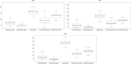
Table 1. Simulation results of MEDIAN, TP, FP, CORRECT and ME for Example 4.1.

p	Method	MEDIAN	TP	FP	CORRECT	ME
	ISIS-Group-Lasso	6.00	4.00 (0.00)	2.88 (2.99)	0.12	2.19 (0.32)
p=200	g-ISIS-Group-Lasso	4.00	4.00 (0.00)	0.76 (0.75)	0.51	1.90 (0.38)
	Group Lasso	16.00	4.00 (0.00)	11.78 (2.24)	0.00	2.82 (0.36)
	DC-SIS-Group-Lasso	9.00	3.13 (0.00)	5.76 (2.24)	0.00	4.05 (0.28)
	DC-ISIS-Group-Lasso	13.00	4.00 (0.00)	8.52 (2.24)	0.00	2.73 (0.35)
	ISIS-Group-Lasso	7.00	4.00 (0.00)	3.43 (2.99)	0.09	2.30 (0.39)
p=400	g-ISIS-Group-Lasso	4.00	4.00 (0.00)	0.76 (0.75)	0.51	1.92 (0.46)
	Group Lasso	20.00	4.00 (0.00)	16.11 (2.24)	0.00	2.93 (0.38)
	DC-SIS-Group-Lasso	11.00	3.09 (0.00)	7.48 (2.24)	0.00	4.15 (0.29)
	DC-ISIS-Group-Lasso	14.00	4.00 (0.00)	10.17 (1.49)	0.00	2.77 (0.33)
	ISIS-Group-Lasso	7.00	4.00 (0.00)	3.32 (2.99)	0.14	2.34 (0.49)
p=1000	g-ISIS-Group-Lasso	4.00	3.99 (0.00)	0.83 (0.75)	0.51	1.97 (0.50)
	Group Lasso	28.00	4.00 (0.00)	24.15 (2.99)	0.00	3.02 (0.32)
	DC-SIS-Group-Lasso	13.00	3.04 (0.00)	9.81 (2.24)	0.00	4.17 (0.24)
	DC-ISIS-Group-Lasso	16.00	4.00 (0.00)	11.80 (2.24)	0.00	2.80 (0.32)

Note: Robust standard deviations are given in parentheses. ($\sigma =5$, SNR= 2.92.)

Table 2. Simulation results of MEDIAN, TP, FP, CORRECT and ME for Example 4.2.

p	Method	MEDIAN	TP	FP	CORRECT	ME
	ISIS-Group-Lasso	10.00	8.00 (0.00)	2.89 (2.24)	0.12	1.81 (0.34)
p=200	g-ISIS-Group-Lasso	8.00	8.00 (0.00)	0.73 (0.75)	0.52	1.58 (0.33)
	Group Lasso	34.00	8.00 (0.00)	26.44 (3.73)	0.00	2.74 (0.33)
	DC-SIS-Group-Lasso	19.00	6.22 (0.75)	13.23 (2.24)	0.00	4.40 (1.04)
	DC-ISIS-Group-Lasso	23.00	7.94 (0.00)	14.85 (2.24)	0.00	3.15 (0.44)
	ISIS-Group-Lasso	11.00	8.00 (0.00)	3.08 (2.99)	0.13	1.87 (0.37)
p=400	g-ISIS-Group-Lasso	9.00	8.00 (0.00)	0.87 (0.75)	0.44	1.66 (0.33)
	Group Lasso	45.00	8.00 (0.00)	36.86 (3.73)	0.00	2.95 (0.31)
	DC-SIS-Group-Lasso	21.00	5.47 (0.75)	15.39 (2.24)	0.00	4.99 (0.79)
	DC-ISIS-Group-Lasso	25.00	7.90 (0.00)	17.33 (2.24)	0.00	3.35 (0.43)
	ISIS-Group-Lasso	11.00	8.00 (0.00)	3.37 (2.99)	0.12	1.92 (0.43)
p=1000	g-ISIS-Group-Lasso	8.00	8.00 (0.00)	0.83 (0.75)	0.51	1.66 (0.43)
	Group Lasso	60.00	7.99 (0.00)	52.18 (3.92)	0.00	3.13 (0.33)
	DC-SIS-Group-Lasso	24.00	4.86 (0.75)	19.02 (2.99)	0.00	5.29 (0.62)
	DC-ISIS-Group-Lasso	27.00	7.78 (0.00)	19.43 (2.24)	0.00	3.50 (0.47)

Note: Robust standard deviations are given in parentheses. ($\sigma =4$, SNR= 5.34.)

Table 3. Simulation results of MEDIAN, TP, FP, CORRECT and ME for Example 4.3.

p	Method	MEDIAN	TP	FP	CORRECT	ME
	ISIS-Group-Lasso	7.00	4.00 (0.00)	2.87 (2.24)	0.12	1.64 (0.32)
p=200	g-ISIS-Group-Lasso	4.00	4.00 (0.00)	0.75 (0.75)	0.56	1.37 (0.35)
	Group Lasso	19.00	4.00 (0.00)	15.42 (2.24)	0.00	2.15 (0.28)
	DC-SIS-Group-Lasso	12.00	3.68 (0.75)	8.33 (2.43)	0.00	2.41 (0.67)
	DC-ISIS-Group-Lasso	13.00	4.00 (0.00)	8.73 (1.49)	0.00	2.03 (0.27)
	ISIS-Group-Lasso	6.00	4.00 (0.00)	2.88 (2.24)	0.14	1.64 (0.43)
p=400	g-ISIS-Group-Lasso	4.00	4.00 (0.00)	0.74 (0.75)	0.56	1.37 (0.40)
	Group Lasso	27.00	3.99 (0.00)	22.86 (2.99)	0.00	2.22 (0.26)
	DC-SIS-Group-Lasso	13.00	3.51 (0.75)	9.25 (2.24)	0.00	2.64 (0.71)
	DC-ISIS-Group-Lasso	14.00	4.00 (0.00)	9.88 (1.49)	0.00	2.07 (0.28)
	ISIS-Group-Lasso	7.00	4.00 (0.00)	3.20 (2.99)	0.10	1.77 (0.37)
p=1000	g-ISIS-Group-Lasso	5.00	3.99 (0.00)	0.79 (0.75)	0.44	1.47 (0.41)
	Group Lasso	40.00	4.00 (0.00)	36.01 (3.17)	0.00	2.33 (0.26)
	DCS-Group-Lasso	15.00	3.43 (0.75)	11.71 (2.24)	0.00	2.71 (0.56)
	DC-ISIS-Group-Lasso	15.00	4.00 (0.00)	11.53 (2.24)	0.00	2.15 (0.26)

Note: Robust standard deviations are given in parentheses. ($\sigma =4$, SNR= 2.69.)

Table 4. Simulation results of MEDIAN, TP, FP, CORRECT and ME for Example 4.4.

p	Method	MEDIAN	TP	FP	CORRECT	ME
	ISIS-Group-Lasso	11.00	8.00 (0.00)	3.45 (2.99)	0.13	2.08 (0.43)
p=200	g-ISIS-Group-Lasso	9.00	8.00 (0.00)	0.79 (0.75)	0.46	1.80 (0.32)
	Group Lasso	30.00	8.00 (0.00)	22.17 (2.99)	0.00	3.15 (0.30)
	DC-SIS-Group-Lasso	14.00	5.70 (0.75)	8.08 (2.99)	0.00	5.53 (0.91)
	DC-ISIS-Group-Lasso	18.00	7.52 (0.75)	10.23 (2.24)	0.00	3.52 (1.16)
	ISIS-Group-Lasso	11.00	8.00 (0.00)	3.96 (2.24)	0.07	2.19 (0.38)
p=400	g-ISIS-Group-Lasso	9.00	7.98 (0.00)	0.79 (0.75)	0.49	1.86 (0.34)
	Group Lasso	37.00	7.97 (0.00)	29.55 (3.17)	0.00	3.35 (0.41)
	DC-SIS-Group-Lasso	14.00	5.26 (0.75)	8.99 (2.24)	0.00	5.87 (0.82)
	DC-ISIS-Group-Lasso	18.00	7.44 (0.75)	11.25 (2.99)	0.00	3.69 (1.12)
	ISIS-Group-Lasso	11.00	8.00 (0.00)	3.91 (2.24)	0.07	2.24 (0.39)
p=1000	g-ISIS-Group-Lasso	8.00	7.94 (0.00)	0.75 (0.75)	0.50	1.92 (0.34)
	Group Lasso	49.00	7.91 (0.00)	40.75 (4.48)	0.00	3.60 (0.36)
	DC-SIS-Group-Lasso	16.00	4.88 (0.75)	11.19 (2.99)	0.00	6.07 (0.54)
	DC-ISIS-Group-Lasso	20.00	7.40 (0.75)	12.77 (2.24)	0.00	3.77 (1.11)

Note: Robust standard deviations are given in parentheses. ($\sigma =4$, SNR= 6.78.)

4.2. Real example

In this section, we compare ISIS-Group-Lasso, g-ISIS-Group-Lasso and Group-Lasso on colon data (Alon et al., 1999). Alon's work reports the application of a two-way clustering method for analysis a data set consisting of the expression patterns of different cell types. For these data, we were interested in finding the genes that are related to colon tumour. In the original colon data, the identity of the 62 samples from colon-cancer patients were analysed with an Affymetrix oligonucleotide Hum6000 array. And these data contain the expression of the 2000 genes with the highest minimal intensity across the 62 tissues, where the genes are placed in order of descending minimal intensity. That is, the original data have 2000 numerical variables. For each continuous variable in the additive model, we use five B-spline basis functions to represent its effect, which is originally used by Yang and Zou (2015) in solving group-lasso penalise learning problems. Thus we obtain 10,000 predictors in 2000 groups after basis function expansion. Three methods are used to select relevant additive components.

Before the analysis, all data are standardised in advance such that each variable has zero mean and unit sample variance. To valuate the performance of the three methods, we used cross-validation and compared the average model size (AMS) and the prediction mean squared error (PE). We randomly partitioned the data into a training data set of 50 observations and a test set of 12 observations. That is, we conduct group screening using 50 observations and the PEs on these 12 test sets. Detailed results based on 100 replications are presented in Table 5. In addition, the boxplot of the average model size is presented in Figure 2. As clearly shown in Table 5, ISIS-Group-Lasso and g-ISIS-Group-Lasso select far fewer genes than Group-Lasso, while the first two methods have a smaller PE. In conclusion, the proposed iterative group screening approach is very useful in high-dimensional scientific studies, which can select a parsimonious model and reveal interesting relationship between group variables.

Figure 2. Boxplot of average model sizes for colon data analysis.

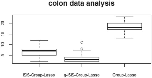
Table 5. Results of AMS and CORRECT for colon data.

Method	AMS	PE
ISIS-Group-Lasso	6.58 (2.24)	2.08 (0.34)
g-ISIS-Group-Lasso	3.6 (1.49)	2.10 (0.35)
Group Lasso	18.49 (2.24)	3.09 (0.58)

Note: Robust standard deviations are given in parentheses.

5. Concluding remarks

In this article, we have proposed the marginal group sure screening method under the context of ultra-high dimensionality. Unlike most existing literatures, we deal with variables, which can be naturally grouped. Our group screening method respects the grouping structure in the data and is based on a working independence. Theoretically, we establish the sure screening property for this group screening approach. To enhance the finite sample performance, a data-driven thresholding and an iterative procedure, ISIS-Group-Lasso, are developed. A greedy modification to the iterative procedure, g-ISIS-Group-Lasso is also proposed to further reduce the false positive. Simulation results show that these two methods perform well in terms of the five performance measures.

This article leaves the problems of extending the ISIS-Group-Lasso and g-ISIS-Group-Lasso under linear model to the family of generalised linear model and other parametric models. And model-free group screening approach may be appealing for dealing with ultra-high-dimensional data more generally, which avoids the difficult task of specifying the form of a statistical model. These problems are beyond the scopes of this article and are interesting topics for future research.

Disclosure statement

No potential conflict of interest was reported by the authors.

Additional information

Funding

This research was supported by the National Natural Science Foundation of China (CN) (11571112), the National Social Science Foundation Key Program (17ZDA091) and Natural Science Fund of Education Department of Anhui Province (KJ2013B233), the 111 Project of China (B14019).

Notes on contributors

Yong Niu

Yong Niu is a PhD candidate in the College of Statistics, East China Normal University, Shanghai, China. His research interests include high dimensional data, big data analytics and nonparametric statistics.

Riquan Zhang

Riquan Zhang is a professor and chair of School of Statistics in East China Normal University. His research interests include high dimensional data, big data analytics, functional data analysis, statistical machine learning and nonparametric statistics.

Jicai Liu

Jicai Liu is an associate professor of statistics in the department of mathematics at Shanghai Normal University, China. His research interests include high dimensional data, lifetime data analysis and nonparametric statistics.

Huapeng Li

Huapeng Li is an associate professor of statistics in the school of mathematics and statistics at Datong University, China. His research interests include nonparametric and semiparametric statistics based on empirical likelihood, selection biased data and finite mixture models.

Appendix 1.

Three lemmas

Next, we state some lemmas which will be used in the proof of Theorems 3.1 and 3.2.

Lemma A.1

Under conditions (i)–(iii), for any $\delta >0,$ $j=1,2,\dots ,J,$ we have $\begin{array}{rl}& P\left\{\frac{1}{\sqrt{p_j}}∥\frac{1}{n}{\mathit{x}}_j^{\mathrm{T}}\mathit{y}-E{\mathit{X}}_{j}Y∥\ge \frac{\delta }{n}\right\}\\ & \le 4p_j\exp \{-{\delta }^2/(c_{2}n+c_3\delta \left)\right\},\end{array}$ where $c_2=max(8M_0^2{M}_1,16M_2)$ and $c_3=max\left(\frac{1}{3}{M}_0{M}_1,1\right).$

Proof.

Using Bonferroni's inequality, we can easily prove that $\begin{array}{rl}& P\left\{\frac{1}{\sqrt{p_j}}∥\frac{1}{n}{\mathit{x}}_j^{\mathrm{T}}\mathit{y}-E{\mathit{X}}_{j}Y∥\ge \frac{\delta }{n}\right\}\\ & \le P\left\{\bigcup _{k=1}^{p_j}\left({\left[\frac{1}{n}\sum _{i=1}^n(x_{ijk}{y}_i-E{X}_{jk}Y)\right]}^2\ge \frac{{\delta }^2}{n^2}\right)\right\}\\ & \le \sum _{k=1}^{p_j}P\left\{\left|\sum _{i=1}^n(x_{ijk}{y}_i-E{X}_{jk}Y)\right|\ge \delta \right\}.\end{array}$ Thus we need to show that $P\left\{\left|\sum _{i=1}^n(x_{ijk}{y}_i-E{X}_{jk}Y)\right|\ge \delta \right\}\le 4\exp \{-{\delta }^2/(c_{2}n+c_3\delta \left)\right\},$ for every $k=1,2,\dots ,p_j.$ Recall that the support of $X_{jk}$ is $[a,b]$ for $j=1,2,\dots ,J$ and $k=1,2,\dots ,p_j,$ we denote $M_0=max(|a|,|b|).$ Because $y_i=\sum _{j=1}^J{\mathbf{x}}_{ij}^{\mathrm{T}}{\beta }_j+{\epsilon }_i,$ we can obtain that $\begin{array}{rl}{x}_{ijk}{y}_i-E{X}_{jk}Y& =\left\{x_{ijk}\left(\sum _{j=1}^J{\mathit{x}}_{ij}^{\mathrm{T}}{\mathit{\beta }}_j\right)-E\left[x_{ijk}\left(\sum _{j=1}^J{\mathit{x}}_{ij}^{\mathrm{T}}{\mathit{\beta }}_j\right)\right]\right\}\\ & +x_{ijk}{\epsilon }_i\\ & \widehat{=}{S}_{ijk1}+S_{ijk2}.\end{array}$ Next we bound the tails probability of $|S_{ijk1}|$ and $|S_{ijk2}|$ respectively. By condition (ii)–(iii), it is easy to see that $\begin{array}{rl}|S_{ijk1}|& \le M_0{M}_1,\\ \mathrm{V}\mathrm{a}\mathrm{r}\left(S_{ijk1}\right)& \le M_0^2{M}_1^2,\\ E|S_{ijk2}{|}^m& \le E{M}_0^m|{\epsilon }_i{|}^m\\ & \le m!E\exp M_0|{\epsilon }_i|\le M_{2}m!(m\ge 2).\end{array}$ Using the Bernstein's inequality (Van der Vaart & Wellner, 1996, lemma 2.2.9 and lemma 2.2.11), we conclude that (A1) $\begin{array}{r}P\left\{\left|\sum _{i=1}^n{S}_{ijk1}\right|>\frac{\delta }{2}\right\}\le 2\exp \left\{-\frac{{\delta }^2}{8}\frac{1}{n{M}_0^2{M}_1^2+M_0{M}_1\delta /6}\right\},\end{array}$(A1) (A2) $\begin{array}{r}P\left\{\left|\sum _{i=1}^n{S}_{ijk2}\right|>\frac{\delta }{2}\right\}\le 2\exp \left\{-\frac{{\delta }^2}{8}\frac{1}{2n{M}_2+\delta /2}\right\}.\end{array}$(A2) Therefore, we combine the results (A1(A1) $\begin{array}{r}P\left\{\left|\sum _{i=1}^n{S}_{ijk1}\right|>\frac{\delta }{2}\right\}\le 2\exp \left\{-\frac{{\delta }^2}{8}\frac{1}{n{M}_0^2{M}_1^2+M_0{M}_1\delta /6}\right\},\end{array}$(A1) ) and (A2(A2) $\begin{array}{r}P\left\{\left|\sum _{i=1}^n{S}_{ijk2}\right|>\frac{\delta }{2}\right\}\le 2\exp \left\{-\frac{{\delta }^2}{8}\frac{1}{2n{M}_2+\delta /2}\right\}.\end{array}$(A2) ) with $c_2=max(8M_0^2{M}_1,16M_2)$ and $c_3=max\left(\frac{1}{3}{M}_0{M}_1,1\right)$, to obtain that $P\left\{\left|\sum _{i=1}^n(x_{ijk}{y}_i-E{X}_{jk}Y)\right|\ge \delta \right\}\le 4\exp \{-{\delta }^2/(c_{2}n+c_3\delta \left)\right\}.$ This concludes the proof of the lemma.

Lemma A.2

Under conditions (ii)–(iv), for any $\delta >0$ and $j=1,2,\dots ,J$, we have $P\left\{\frac{1}{p_j}∥\frac{1}{n}{\mathit{x}}_j^{\mathrm{T}}{\mathit{x}}_j-E{\mathit{X}}_j{\mathit{X}}_j^{\mathrm{T}}∥\ge \frac{1}{n}\delta \right\}\le 2p_j^2\exp \left\{-\frac{{\delta }^2}{c_{4}n+c_5\delta }\right\}$ where $c_4=2M_0^4$ and $c_5=\frac{4M_0^2}{3}$.

Proof.

For $s=1,2,\dots ,p_j,t=1,2,\dots ,p_j$, let $T_j=\frac{1}{n}{\mathit{x}}_j^{\mathrm{T}}{\mathbf{x}}_j-E{X}_j{X}_j^{\mathrm{T}}$ and $T_j^{(s,t)}$ be the entry of $T_j$. Then we can write $T_j^{(s,t)}=\frac{1}{n}\sum _{i=1}^n(x_{ijs}{x}_{ijt}-E{X}_{js}{X}_{jt}).$

By the fact that $\parallel A\parallel \le p\parallel A{\parallel }_{\mathrm{\infty }}$, we have (A3) $\begin{array}{rl}& P\left\{\frac{1}{p_j}∥\frac{1}{n}{\mathit{x}}_j^{\mathrm{T}}{\mathit{x}}_j-E{\mathit{X}}_j{\mathit{X}}_j^{\mathrm{T}}∥\ge \frac{1}{n}\delta \right\}\\ & \le P\left\{{∥\frac{1}{n}{\mathit{x}}_j^{\mathrm{T}}{\mathit{x}}_j-E{\mathit{X}}_j{\mathit{X}}_j^{\mathrm{T}}∥}_{\mathrm{\infty }}\ge \frac{1}{n}\delta \right\}\\ & \le \sum _{s=1}^{p_j}\sum _{t=1}^{p_j}P\left\{|T_j^{(s,t)}|\ge \frac{\delta }{n}\right\}.\end{array}$(A3) Next we also use Bernstein's inequality to bound the tails probability of $T_j^{(s,t)}$. By condition (ii)–(iii), we can obtain easily that $\begin{array}{rl}|x_{ijs}{x}_{ijt}-E{X}_{js}{X}_{jt}|& \le 2M_0^2,\\ \mathrm{V}\mathrm{a}\mathrm{r}\left(x_{ijs}{x}_{ijt}\right)& \le M_0^4.\end{array}$ Using Bernstein's inequality, it follows that (A4) $P\left\{|T_j^{(s,t)}|\ge \frac{\delta }{n}\right\}\le 2\exp \left\{-\frac{1}{2}\frac{{\delta }^2}{n{M}_0^4+2M_0^2\delta /3}\right\}.$(A4) Thus the desired result is obtained from (A3(A3) $\begin{array}{rl}& P\left\{\frac{1}{p_j}∥\frac{1}{n}{\mathit{x}}_j^{\mathrm{T}}{\mathit{x}}_j-E{\mathit{X}}_j{\mathit{X}}_j^{\mathrm{T}}∥\ge \frac{1}{n}\delta \right\}\\ & \le P\left\{{∥\frac{1}{n}{\mathit{x}}_j^{\mathrm{T}}{\mathit{x}}_j-E{\mathit{X}}_j{\mathit{X}}_j^{\mathrm{T}}∥}_{\mathrm{\infty }}\ge \frac{1}{n}\delta \right\}\\ & \le \sum _{s=1}^{p_j}\sum _{t=1}^{p_j}P\left\{|T_j^{(s,t)}|\ge \frac{\delta }{n}\right\}.\end{array}$(A3) ) and (A4(A4) $P\left\{|T_j^{(s,t)}|\ge \frac{\delta }{n}\right\}\le 2\exp \left\{-\frac{1}{2}\frac{{\delta }^2}{n{M}_0^4+2M_0^2\delta /3}\right\}.$(A4) ) by taking $c_4=2M_0^4$ and $c_5=\frac{4M_0^2}{3}$.

Remark A.1

If A and B are two symmetric matrices of order p, we have the following two results (Fan, Feng, & Song, 2011; He et al., 2013): $\begin{array}{rl}& |{\lambda }_{min}\left(A\right)-{\lambda }_{min}\left(B\right)|\le max\left\{|{\lambda }_{min}\right(A-B)|,{\lambda }_{min}(B-A\left)|\right\},\\ & |{\lambda }_{max}\left(A\right)-{\lambda }_{max}\left(B\right)|\le max\left\{|{\lambda }_{max}\right(A-B)|,{\lambda }_{max}(B-A\left)|\right\}.\end{array}$ In addition, note that $|{\lambda }_{min}(A-B)|\le |{\lambda }_{max}(A-B)|\le p\parallel A-B{\parallel }_{\mathrm{\infty }}.$ The above results, together with Lemma 2, imply that (A5) $\begin{array}{rl}& P\left\{\left|{\lambda }_{min}\left(\frac{1}{n}{\mathit{x}}_j^{\mathrm{T}}{\mathit{x}}_j\right)-{\lambda }_{min}\left(E{\mathit{X}}_j{\mathit{X}}_j^{\mathrm{\prime }}\right)\right|\ge \frac{p_j}{n}\delta \right\}\\ & \le 2p_j^2\exp \left\{-\frac{{\delta }^2}{c_{4}n+c_5\delta }\right\},\end{array}$(A5) (A6) $\begin{array}{rl}& P\left\{\left|{\lambda }_{max}\left(\frac{1}{n}{\mathit{x}}_j^{\mathrm{T}}{\mathit{x}}_j\right)-{\lambda }_{max}\left(E{\mathit{X}}_j{\mathit{X}}_j^{\mathrm{T}}\right)\right|\ge \frac{p_j}{n}\delta \right\}\\ & \le 2p_j^2\exp \left\{-\frac{{\delta }^2}{c_{4}n+c_5\delta }\right\}\end{array}$(A6) for $j=1,2,\dots ,p_j$.

Lemma A.3

Suppose conditions (ii)–(iv) hold, there exist some positive constants ${\tau }_3$ and ${\tau }_4$ such that (A7) $\begin{array}{rl}& P\left\{{\tau }_3\le {\lambda }_{min}\left(\frac{1}{n}{\mathit{x}}_j^{\mathrm{T}}{\mathit{x}}_j\right)\le {\lambda }_{max}\left(\frac{1}{n}{\mathit{x}}_j^{\mathrm{T}}{\mathit{x}}_j\right)\le {\tau }_4\right\}\\ & \ge 1-2p_j^2\exp \left\{-\frac{{\delta }^2}{c_{4}n+c_5\delta }\right\}.\end{array}$(A7) That is, with probability approaching 1, we have $0<{\tau }_3\le {\lambda }_{min}\left(\frac{1}{n}{\mathit{x}}_j^{\mathrm{T}}{\mathit{x}}_j\right)\le {\lambda }_{max}\left(\frac{1}{n}{\mathit{x}}_j^{\mathrm{T}}{\mathit{x}}_j\right)\le {\tau }_4<\mathrm{\infty }.$

Proof.

Combing condition (iv) and (A5(A5) $\begin{array}{rl}& P\left\{\left|{\lambda }_{min}\left(\frac{1}{n}{\mathit{x}}_j^{\mathrm{T}}{\mathit{x}}_j\right)-{\lambda }_{min}\left(E{\mathit{X}}_j{\mathit{X}}_j^{\mathrm{\prime }}\right)\right|\ge \frac{p_j}{n}\delta \right\}\\ & \le 2p_j^2\exp \left\{-\frac{{\delta }^2}{c_{4}n+c_5\delta }\right\},\end{array}$(A5) )–(A6(A6) $\begin{array}{rl}& P\left\{\left|{\lambda }_{max}\left(\frac{1}{n}{\mathit{x}}_j^{\mathrm{T}}{\mathit{x}}_j\right)-{\lambda }_{max}\left(E{\mathit{X}}_j{\mathit{X}}_j^{\mathrm{T}}\right)\right|\ge \frac{p_j}{n}\delta \right\}\\ & \le 2p_j^2\exp \left\{-\frac{{\delta }^2}{c_{4}n+c_5\delta }\right\}\end{array}$(A6) ), it is easy to obtain (A7(A7) $\begin{array}{rl}& P\left\{{\tau }_3\le {\lambda }_{min}\left(\frac{1}{n}{\mathit{x}}_j^{\mathrm{T}}{\mathit{x}}_j\right)\le {\lambda }_{max}\left(\frac{1}{n}{\mathit{x}}_j^{\mathrm{T}}{\mathit{x}}_j\right)\le {\tau }_4\right\}\\ & \ge 1-2p_j^2\exp \left\{-\frac{{\delta }^2}{c_{4}n+c_5\delta }\right\}.\end{array}$(A7) ).

Appendix 2.

Proof of Theorem 3.1

Proof of Theorem 3.1.

The key idea of the proof is to show the uniform consistence of $\parallel {\hat{\upsilon }}_{nj}{\parallel }_n^2$ under conditions (ii)–(iv). As to the existing literatures, the sure screening property is typically established in this way. Recall that $\parallel {\hat{\upsilon }}_{nj}{\parallel }_n^2={\left(\frac{1}{n}{\mathit{x}}_j^{\mathrm{T}}\mathit{y}\right)}^{\mathrm{T}}{\left(\frac{1}{n}{\mathit{x}}_j^{\mathrm{T}}{\mathit{x}}_j\right)}^{-1}\left(\frac{1}{n}{\mathit{x}}_j^{\mathrm{T}}\mathit{y}\right)$ and $\parallel {\upsilon }_j{\parallel }^2=\left(E{\mathit{X}}_{j}Y{)}^{\mathrm{T}}\right(E{\mathit{X}}_j{\mathit{X}}_j^{\mathrm{T}}{)}^{-1}\left(E{\mathit{X}}_{j}Y\right).$ Thus we need to evaluate $\begin{array}{rl}\frac{1}{p_j}\parallel {\hat{\upsilon }}_{nj}{\parallel }_n^2-\frac{1}{p_j}\parallel {\upsilon }_j{\parallel }^2& =\frac{1}{p_j}{\left(\frac{1}{n}{\mathit{x}}_j^{\mathrm{T}}\mathit{y}\right)}^{\mathrm{T}}{\left(\frac{1}{n}{\mathit{x}}_j^{\mathrm{T}}{\mathit{x}}_j\right)}^{-1}\left(\frac{1}{n}{\mathit{x}}_j^{\mathrm{T}}\mathit{y}\right)\\ & -\frac{1}{p_j}\left(E{\mathit{X}}_{j}Y{)}^{\mathrm{T}}\right(E{\mathit{X}}_j{\mathit{X}}_j^{\mathrm{T}}{)}^{-1}\left(E{\mathit{X}}_{j}Y\right).\end{array}$ By some algebra, we decompose it into three parts $\parallel {\hat{\upsilon }}_{nj}{\parallel }_n^2-\parallel {\upsilon }_j{\parallel }^2={\lambda }_1+{\lambda }_2+{\lambda }_3$ in which $\begin{array}{rl}& {\lambda }_1={\left(\frac{1}{n}{\mathit{x}}_j^{\mathrm{T}}\mathit{y}-E{\mathit{X}}_{j}Y\right)}^{\mathrm{T}}{\left(\frac{1}{n}{\mathit{x}}_j^{\mathrm{T}}{\mathit{x}}_j\right)}^{-1}\left(\frac{1}{n}{\mathit{x}}_j^{\mathrm{T}}\mathit{y}-E{\mathit{X}}_{j}Y\right),\\ & {\lambda }_2={\left(\frac{1}{n}{\mathit{x}}_j^{\mathrm{\prime }}\mathit{y}-E{\mathit{X}}_{j}Y\right)}^{\mathrm{T}}{\left(\frac{1}{n}{\mathit{x}}_j^{\mathrm{T}}{\mathit{x}}_j\right)}^{-1}E{\mathit{X}}_{j}Y,\\ & {\lambda }_3=\left(E{\mathit{X}}_{j}Y{)}^{\mathrm{T}}{\left(\frac{1}{n}{\mathit{x}}_j^{\mathrm{T}}{\mathit{x}}_j\right)}^{-1}\right(E{\mathit{X}}_j{\mathit{X}}_j^{\mathrm{T}}\\ & -\frac{1}{n}{\mathit{x}}_j^{\mathrm{T}}{\mathit{x}}_j\left)\right(E{\mathit{X}}_j{\mathit{X}}_j^{\mathrm{T}}{)}^{-1}E{\mathit{X}}_{j}Y.\end{array}$ Now, we define a event ${\mathrm{\Omega }}_{\delta }$ on which we have $\begin{array}{rl}& \frac{1}{\sqrt{p_j}}∥\frac{1}{n}{\mathit{x}}_j^{\mathrm{T}}\mathit{y}-E{\mathit{X}}_{j}Y∥\le \frac{\delta }{n},\\ & \frac{1}{p_j}∥\frac{1}{n}{\mathit{x}}_j^{\mathrm{T}}{\mathit{x}}_j-E{\mathit{X}}_j{\mathit{X}}_j^{\mathrm{T}}∥\le \frac{1}{n}\delta ,\\ & {\tau }_3\le {\lambda }_{min}\left(\frac{1}{n}{\mathit{x}}_j^{\mathrm{T}}{\mathit{x}}_j\right)\le {\lambda }_{max}\left(\frac{1}{n}{\mathit{x}}_j^{\mathrm{T}}{\mathit{x}}_j\right)\le {\tau }_4\end{array}$ for $j=1,2,\dots ,J$.

Then the above three lemmas indicate that (A8) $\begin{array}{rl}P\left({\mathrm{\Omega }}_{\delta }\right)& \ge 1-4\sum _{j=1}^J{p}_j\exp \{-{\delta }^2/(c_{2}n+c_3\delta \left)\right\}\\ & -4\sum _{j=1}^J{p}_j^2\exp \{-{\delta }^2/(c_{4}n+c_5\delta \left)\right\}.\end{array}$(A8) By the fact that $\parallel AB\parallel \le \parallel A\parallel \parallel B\parallel$, we have on ${\mathrm{\Omega }}_{\delta }$, $\begin{array}{rl}\frac{1}{p_j}|{\lambda }_1|& \le {∥\frac{1}{n}{\mathit{x}}_j^{\mathrm{T}}\mathit{Y}-E{\mathit{X}}_{j}Y∥}^2∥{\left(\frac{1}{n}{\mathit{x}}_j^{\mathrm{T}}{\mathit{x}}_j\right)}^{-1}∥\le \frac{{\delta }^2}{n^2}\frac{1}{{\tau }_3},\\ \frac{1}{p_j}|{\lambda }_2|& \le 2∥\frac{1}{n}{\mathit{x}}_j^{\mathrm{T}}\mathit{y}-E{\mathit{X}}_{j}Y∥∥{\left(\frac{1}{n}{\mathit{x}}_j^{\mathrm{T}}{\mathit{x}}_j\right)}^{-1}∥\\ \parallel E{\mathit{X}}_{j}Y\parallel & \le \frac{\delta }{n}\frac{2M_0{M}_1}{{\tau }_3},\\ \frac{1}{p_j}|{\lambda }_3|& \le ∥{\left(\frac{1}{n}{\mathit{x}}_j^{\mathrm{T}}{\mathit{x}}_j\right)}^{-1}∥\parallel (E{\mathit{X}}_j{\mathit{X}}_j^{\mathrm{T}}{)}^{-1}\parallel ∥E{\mathit{X}}_j{\mathit{X}}_j^{\mathrm{T}}-\frac{1}{n}{\mathit{x}}_j^{\mathrm{T}}{\mathit{x}}_j∥\\ \parallel E{\mathit{X}}_{j}Y{\parallel }^2& \le \frac{\delta }{n}\frac{M_0{M}_1}{{\tau }_1{\tau }_3}.\end{array}$ Take $\delta =c_6{n}^{1-\kappa }$, there exists a constant $c_7$ such that $\frac{{\delta }^2}{n^2}\frac{1}{{\tau }_3}+\frac{\delta }{n}\frac{2M_0{M}_1}{{\tau }_3}+\frac{\delta }{n}\frac{M_0{M}_1}{{\tau }_1{\tau }_3}\le c_6{c}_7{n}^{-\kappa }.$ Choosing $c_6$ such that $c_6{c}_7\le c$, we can easily obtain that $\left|{∥\frac{1}{p_j}{\hat{\upsilon }}_{nj}∥}_n^2-\frac{1}{p_j}\parallel {\upsilon }_j{\parallel }^2\right|\le c{n}^{-\kappa }.$ By invoking condition (i), we have on ${\mathrm{\Omega }}_{\delta }$ for sufficiently large n ${∥\frac{1}{p_j}{\hat{\upsilon }}_{nj}∥}_n^2\ge 2c{n}^{-\kappa }.$ If we choose ${\pi }_n\le 2c{n}^{-\kappa }$, it is easy to show that $j\in {\mathcal{M}}_{\ast }.$ This, together with (A8(A8) $\begin{array}{rl}P\left({\mathrm{\Omega }}_{\delta }\right)& \ge 1-4\sum _{j=1}^J{p}_j\exp \{-{\delta }^2/(c_{2}n+c_3\delta \left)\right\}\\ & -4\sum _{j=1}^J{p}_j^2\exp \{-{\delta }^2/(c_{4}n+c_5\delta \left)\right\}.\end{array}$(A8) ), indicates that there exists a constant $c_1$ such that $P\{{\mathcal{M}}_{\ast }\subset \widehat{{\mathcal{M}}_{\kappa }}\}\ge 1-4\sum _{j=1}^J(p_j+p_j^2)\exp \{-c_1{n}^{1-2\kappa }\}.$

Appendix 3.

Proof of Theorem 3.2

Proof of Theorem 3.2.

Following the similar argument of the proof of Theorem 3.1, we have on ${\mathrm{\Omega }}_{\delta }$ $\begin{array}{rl}& \left|\left\{1\le j\le J:\frac{1}{p_j}\parallel {\hat{\upsilon }}_{nj}{\parallel }_n^2\ge 2c{n}^{-\kappa }\right\}\right|\\ & \le \left|\left\{1\le j\le J:\frac{1}{p_j}\parallel {\upsilon }_j{\parallel }^2\ge c{n}^{-\kappa }\right\}\right|,\end{array}$ where $|.|$ denotes the size of the set. This implies that $\sum _{j\in \widehat{{\mathcal{M}}_{\kappa }}}\frac{1}{p_j}\parallel {\upsilon }_j{\parallel }^2\ge c{n}^{-\kappa }|\widehat{{\mathcal{M}}_{\kappa }}|.$ By some algebra, it follows that $|\widehat{{\mathcal{M}}_{\kappa }}|\le O(n^{\kappa }\sum _{j=1}^J\parallel E{\mathit{X}}_{j}Y{\parallel }^2)=O(n^{\kappa }\parallel E\mathit{X}Y{\parallel }^2).$ That is, we have (A9) $\begin{array}{rl}P\{|\widehat{{\mathcal{M}}_{\kappa }}|& \le O(n^{\kappa }\parallel E\mathit{X}Y{\parallel }^2)\}\\ & \ge 1-4\sum _{j=1}^J(p_j+p_j^2)\exp \{-c_1{n}^{1-2\kappa }\}.\end{array}$(A9) Thus the key point is to show that $\parallel E\mathit{X}Y{\parallel }^2=O\left(1\right).$ For this purpose, we consider the following linear regression: $\underset{\mathit{\alpha }}{min}E(Y-{\mathit{X}}^{\mathrm{T}}\mathit{\alpha }{)}^2$

with respect to $\mathit{\alpha }\in {\mathbb{R}}^{\sum _{j=1}^J{p}_j}$. By least square, we can easily obtain that $\parallel E\mathit{X}Y{\parallel }^2={\hat{\mathit{\alpha }}}^{\mathrm{\prime }}\left[E\right({\mathit{X}}^{\mathrm{T}}\mathit{X}){]}^2\hat{\mathit{\alpha }}\le {\lambda }_{max}(\mathrm{\Sigma }\left){\hat{\mathit{\alpha }}}^{\mathrm{\prime }}E\right({\mathit{X}}^{\mathrm{T}}\mathit{X})\hat{\mathit{\alpha }}$ in which $\hat{\mathit{\alpha }}$ is the least square estimator. On the other hand, the orthogonal decomposition of least square implies that $\mathrm{V}\mathrm{a}\mathrm{r}\left(Y\right)=\mathrm{V}\mathrm{a}\mathrm{r}\left({\mathit{X}}^{\mathrm{T}}\hat{\mathit{\alpha }}\right)+\mathrm{V}\mathrm{a}\mathrm{r}(Y-{\mathit{X}}^{\mathrm{T}}\hat{\mathit{\alpha }})$. Because $\mathrm{V}\mathrm{a}\mathrm{r}\left(Y\right)=O\left(1\right)$, we conclude that (A10) $\parallel E\mathit{X}Y{\parallel }^2\le O\left(1\right).$(A10) Combining (A9(A9) $\begin{array}{rl}P\{|\widehat{{\mathcal{M}}_{\kappa }}|& \le O(n^{\kappa }\parallel E\mathit{X}Y{\parallel }^2)\}\\ & \ge 1-4\sum _{j=1}^J(p_j+p_j^2)\exp \{-c_1{n}^{1-2\kappa }\}.\end{array}$(A9) ) and (A10(A10) $\parallel E\mathit{X}Y{\parallel }^2\le O\left(1\right).$(A10) ), the desired result can be easily obtained.

References

- Alon, U., Barkai, N., Notterman, D. A., Gish, K., Ybarra, S., Mack, D., & Levine, A. J. (1999). Broad patterns of gene expression revealed by clustering analysis of tumor and normal colon tissues probed by oligonucleotide arrays. Proceedings of the National Academy of Sciences, 96(12), 6745–6750. doi: 10.1073/pnas.96.12.6745
- Bakin, S. (1999). Adaptive regression and model selection in data mining problems (Ph.D. thesis). Australian National University, Canberra.
- Breheny, P., & Huang, J. (2009). Penalized methods for bi-level variable selection. Statistics and its Interface, 2(3), 369. doi: 10.4310/SII.2009.v2.n3.a10
- Breheny, P., & Huang, J. (2015). Group descent algorithms for nonconvex penalized linear and logistic regression models with grouped predictors. Statistics and Computing, 25(2), 173–187. doi: 10.1007/s11222-013-9424-2
- Fan, J., Feng, Y., & Song, R. (2011). Nonparametric independence screening in sparse ultra-high-dimensional additive models. Journal of the American Statistical Association, 106(494), 544–557. doi: 10.1198/jasa.2011.tm09779
- Fan, J., & Lv, J. (2008). Sure independence screening for ultrahigh dimensional feature space (with discussion). Journal of the Royal Statistical Society, Series B: Statistical Methodology, 70(5), 849–911. doi: 10.1111/j.1467-9868.2008.00674.x
- Fan, J., Samworth, R., & Wu, Y. (2009). Ultrahigh dimensional variable selection: Beyond the linear model. Journal of Machine Learning Research, 10, 1829–1853.
- Fan, J., & Song, R. (2010). Sure independence screening in generalized linear models with NP-dimensionality. Annals of Statistics, 38(6), 3567–3604. doi: 10.1214/10-AOS798
- He, X., Wang, L., & Hong, H. G. (2013). Quantile-adaptive model-free variable screening for high-dimensional heterogeneous data. Annals of Statistics, 41(1), 342–369. doi: 10.1214/13-AOS1087
- Huang, J., Ma, S., Xie, H., & Zhang, C. H. (2009). A group bridge approach for variable selection. Biometrika, 96(2), 339–355. doi: 10.1093/biomet/asp020
- Li, R., Zhong, W., & Zhu, L. (2012). Feature screening via distance correlation learning. Journal of the American Statistical Association, 107(499), 1129–1139. doi: 10.1080/01621459.2012.695654
- Shao, X., & Zhang, J. (2014). Martingale difference correlation and its use in high-dimensional variable screening. The American Statistical Association, 109(507), 1302–1318. doi: 10.1080/01621459.2014.887012
- Van der Vaart, A. W., & Wellner, J. A. (1996). Weak convergence and empirical processes. New York: Springer.
- Wang, H. (2009). Forward regression for ultra-high dimensional variable screening. Journal of the American Statistical Association, 104(488), 1512–1524. doi: 10.1198/jasa.2008.tm08516
- Wei, F., & Huang, J. (2010). Consistent group selection in high-dimensional linear regression. Bernoulli, 16(4), 1369–1384. doi: 10.3150/10-BEJ252
- Yang, Y., & Zou, H. (2015). A fast unified algorithm for solving group-lasso penalize learning problems. Statistics and Computing, 2015(6), 1129–1141. doi: 10.1007/s11222-014-9498-5
- Yuan, M., & Lin, Y. (2006). Model selection and estimation in regression with grouped variables. Journal of the Royal Statistical Society, Series B: Statistical Methodology, 68(1), 49–67. doi: 10.1111/j.1467-9868.2005.00532.x
- Zhang, C. H., & Huang, J. (2008). The sparsity and bias of the lasso selection in high-dimensional linear regression. The Annals of Statistics, 36(4), 1567–1594. doi: 10.1214/07-AOS520
- Zhao, S. D., & Li, Y. (2012). Principled sure independence screening for Cox models with ultra-high-dimensional covariates. Journal of Multivariate Analysis, 105(1), 397–411. doi: 10.1016/j.jmva.2011.08.002
- Zhao, P., Rocha, G., & Yu, B. (2009). The composite absolute penalties family for grouped and hierarchical variable selection. Annals of Statistics, 37(6A), 3468–3497. doi: 10.1214/07-AOS584
- Zhong, W., & Zhu, L.-P. (2015). An iterative approach to distance correlation-based sure independence screening. Journal of Statistical Computation and Simulation, 85(11), 2331–2345. doi: 10.1080/00949655.2014.928820