Domain estimation under informative linkage

ABSTRACT

A standard assumption when modelling linked sample data is that the stochastic properties of the linking process and process underpinning the population values of the response variable are independent of one another. This is often referred to as non-informative linkage. But what if linkage errors are informative? In this paper, we provide results from two simulation experiments that explore two potential informative linking scenarios. The first is where the choice of sample record to link is dependent on the response; and the second is where the probability of correct linkage is dependent on the response. We focus on the important and widely applicable problem of estimation of domain means given linked data, and provide empirical evidence that while standard domain estimation methods can be substantially biased in the presence of informative linkage errors, an alternative estimation method, based on a Gaussian approximation to a maximum likelihood estimator that allows for non-informative linkage error, performs well.

KEYWORDS:

• Non-deterministic data linkage
• exchangeable linkage errors
• informative sampling
• auxiliary information
• domain estimation
• maximum likelihood

1. Introduction

The steady increase in researcher access to large administrative databases this century has meant that the use of linkage to enhance, or even create, data sets for analysis is now ubiquitous. But concerns about the confidentiality of the sources being linked has meant that in many cases the linking is non-deterministic and is carried out by an independent third party, often referred to as Trusted Third Party, or TTP, linkage. In such cases, the analyst using the linked data set has no access to the identifier information used for linkage and so cannot be sure that the outcome of the linkage process is not related to the analytic variables of interest. This creates a dilemma, since all methods that have been suggested for secondary analysis of linked data have, at their core, an assumption that the linkage error process and the stochastic behaviour of the analysis variables are conditionally independent given the known characteristics of the analysis population. This is sometimes referred to as the assumption of non-informative linkage.

In this paper, we explore sensitivity to this assumption when the focus of analysis is the well-known linear model and the linkage is very straightforward, just involving two register databases covering the same target population, with sample values of the response variable sourced from one register and the model covariates from the other. We also restrict our attention to the common situation where the linear model itself is the very simple one that characterises a set of domain means of interest, with all domains exhibiting the same variability. Our approach is empirical rather than theoretical, in the sense that we use small scale simulation to illustrate issues that can arise when the linkage process is actually informative and also describe a realistic data application where informative linkage is plausible.

We focus on two informative linkage scenarios. The first is where the sample inclusion probabilities for the sample of linked records used in analysis depend on the response variable of interest. The second is where the actual linkage process depends on the values of this variable, in the sense that the probabilities of correct linkage depend on them. Other informative linkage scenarios are no doubt feasible, including where both informative linkage scenarios that we address occur together. However, it seems reasonable to start with an examination of each of these two situations separately since they are easily motivated in the context of TTP linkage. When considering the impact of informative linkage on analysis methods that are supposed to correct for linkage error bias in secondary analysis of linked data, we also restrict our attention to two recently described approaches, both based on a simple exchangeable specification for the linkage error model (LEM) that characterises the distribution of the linkage errors. The first of these is described in Section 3.1 and corresponds to modifying the usual estimating equations for the linear model parameters so that they are unbiased under this LEM, while the second, described in Section 3.2, uses a Gaussian approximation to the joint distribution of the data defined by the observed linkages and the correctly linked data to define the maximum likelihood estimator (MLE) under the LEM. The two approaches are mainly distinguished by their use of auxiliary information. The first uses only linked sample data plus knowledge of the LEM parameters, while the second uses this information as well as information about the marginal distributions of the response and the model covariates in the two population registers.

The paper consists of six sections. The next section describes the inferential framework underpinning the results in the paper, along with the two informative linkage mechanisms that we consider. Section 3 then specifies the LEM that we assume, and shows how it can be used to define unbiased estimating equations for the parameters of the linear model of interest as well as an approximate MLE for these parameters. Section 4 sets out results from model-based simulations of the impact of the two informative linkage mechanisms while Section 5 describes a simulation based on a more practical application that evaluates the impact of potential informative linkage and real LEM misspecification on the estimating methods described in Section 3. Section 6 finally concludes the paper with a short discussion of the implications of the results presented in it.

2. The inferential framework

We focus on using linked data from two population registers. In particular, we assume that the covariates X are available from the first register, while the response values are available from the second register. The records making up the registers do not have a common unique identifier, so linkage is non-deterministic, based on shared, but not unique, identifying information about the units making up the population covered by the registers. These identifiers are assumed to have no errors. However, since they are also not unique, linkage based upon them is subject to error. Without loss of generality, we assume that the ordering of records on the first register is the ‘true’ population ordering, with y denoting the correspondingly ordered vector of population values of the response. By definition, y is unknown. However, the population vector ${\mathbf{\text{y}}}^{\ast }$of linked values of the response is supposed to be close (if not equal) to y. The actual population records of interest are then the rows of $\left[\mathbf{\text{y}}\mathbf{\text{X}}\right]$, while their linked version is defined by the rows of $\left[{\mathbf{\text{y}}}^{\ast }\mathbf{\text{X}}\right]$. Finally, we note that in many cases it may be too expensive to completely link both registers, so a sample of records from the first register (i.e., the one defining X) is linked to records in the second register (the one defining y). However, the linking agency is willing to make non-identifying tabulations from both registers available, and these can be used to define auxiliary data for inference.

The linked data analysis methods set out in the following section make a number of further assumptions. These are:

1. Both registers have complete coverage of the same population, with no duplicates;

2. Linkage is one to one, with all records (potentially) linkable, i.e., there are no intrinsically non-linkable records;

3. Error-free common identifiers are available on each register, and allow both to be partitioned into q = 1,..,Q disjoint subsets referred to as blocks in what follows;

4. Records in different blocks can never be linked, so there can be no linkage errors between blocks;

5. Sampling from rows of X and then linking to obtain ${\mathbf{\text{y}}}^{\ast }$ is stochastically equivalent to directly sampling the rows of $\left[{\mathbf{\text{y}}}^{\ast }\mathbf{\text{X}}\right]$. That is, sample then link is stochastically equivalent to link then sample;

6. The auxiliary data consist of the block averages for both y and X.

In addition to these assumptions, it is usually assumed (often implicitly) that the linkage process is non-informative for the population model of interest. That is, linkage errors are independent of analysis errors given covariate information. However, in this paper, we consider the case where linkage is in fact informative. In particular, in the simulations described in Section 4, we consider two potential informative linkage mechanisms.

1. The decision on which record to link is correlated with the value of the response variable Y of interest via a latent variable Z. For example, probability sampling is used to determine which linked register unit to sample, with inclusion probability proportional to the value of a latent variable Z that is correlated with Y.

2. The probability of making a correct link depends on the value of the response variable Y through a latent variable Z. That is, Pr(correct link) = f(Z), where Z is correlated with Y.

In both cases, Z could be thought of as a measure of the amount of high-quality linking information available for a particular population unit. Under TTP linkage this information would not be provided to a secondary analyst working with the linked data, and would, therefore, be latent as far as that analyst is concerned.

3. Modelling under linkage error

Without loss of generality, we confine our attention to the M records making up a single block within the population of interest. We, therefore, drop the block subscript q, with the understanding that all block-specific summations defined below need to be extended to population-specific summations by re-introducing q and summing over this index. Following Chambers (2009), we next note that ${\mathbf{\text{y}}}^{\ast }=\mathbf{\text{A}}\mathbf{\text{y}}$ when linkage is one to one and complete, where $\mathbf{\text{A}}=\left[a_{ij}\right]$ is an unknown latent random permutation matrix of order M, with binary-valued coefficients. This reference also proposes a simple (unrealistic but pragmatic) non-informative linkage error model (LEM) for A for use in secondary analysis. This is the Exchangeable Linkage Errors (ELE) model, defined by $\begin{array}{rl}& Pr\left\{y_i^{\ast }=y_j|\mathbf{\text{X}}\right\}=Pr\left\{a_{ij}=1|\mathbf{\text{X}}\right\}={\lambda }_{ij}\\ & =\left\{\begin{array}{ll}\lambda ,& i=j,\\ \eta ,& i\ne j\end{array}\right.i,j=1,\dots ,M\end{array}$Here, $\lambda$ is a fixed, block-specific, parameter which for the time being is assumed to be known. Also, since linkage is one to one and complete, it is straightforward to see that $\eta =(M-1{)}^{-1}\left(1-\lambda \right)$. Let ${\mathbf{\text{I}}}_M$ denote the identity matrix of order M and ${\mathbf{\text{1}}}_M$ denote a vector of ones of size equal to M. Then $\mathbf{\text{T}}=E\left(\mathbf{\text{A}}|\mathbf{\text{X}}\right)=\left(\lambda -\eta \right){\mathbf{\text{I}}}_M+\eta {\mathbf{\text{1}}}_M{\mathbf{\text{1}}}_M^T$

Sampling corresponds to selecting a subset of m linked records. We assume that this sampling is non-informative given X (e.g., simple random sampling within blocks) and use a subscript of s to denote the set of sampled records. Without loss of generality, we also assume that s consists of the population units making up the first m rows of X. Let ${\mathbf{\text{A}}}_s$ denote the rows of A corresponding to records in s. The linked sample values of the response variable are then ${\mathbf{\text{y}}}_s^{\ast }={\mathbf{\text{A}}}_s\mathbf{\text{y}}$. Finally, we put $\begin{array}{rl}{\mathbf{\text{T}}}_s& =E\left({\mathbf{\text{A}}}_s|\mathbf{\text{X}}\right)\\ & =\left[\begin{array}{ccc}\left(\lambda -\eta \right){\mathbf{\text{I}}}_m+\eta {\mathbf{\text{1}}}_m{\mathbf{\text{1}}}_m^T& |& \eta {\mathbf{\text{1}}}_m{\mathbf{\text{1}}}_{M-m}^T\end{array}\right]\\ & =\left[\begin{array}{cc}{\mathbf{\text{T}}}_{ss}& {\mathbf{\text{T}}}_{sr}\end{array}\right].\end{array}$Here, ${\mathbf{\text{I}}}_m$ denotes the identity matrix of order m and ${\mathbf{\text{1}}}_m$, ${\mathbf{\text{1}}}_{M-m}$ denote vectors of ones of sizes equal to m and M-m respectively.

3.1. Solution of an approximate unbiased estimating equation under ELE

From now on, we assume that our population response and covariate values are related via the simple linear model, $E\left(\mathbf{\text{y}}|\mathbf{\text{X}}\right)=\mathbf{\text{f}}=\mathbf{\text{X}}\beta$ and $Var\left(\mathbf{\text{y}}|\mathbf{\text{X}}\right)={\sigma }^2{\mathbf{\text{I}}}_M$. In this sub-section, we further restrict ourselves to where we only have access to linked sample data $\left\{{\mathbf{\text{y}}}_s^{\ast },{\mathbf{\text{X}}}_s\right\}$, see Kim and Chambers (2012). Under the ELE model, an unbiased estimating equation for $\beta$ is ${\mathbf{\text{G}}}_s\left({\mathbf{\text{y}}}_s^{\ast }-{\mathbf{\text{H}}}_s\beta \right)=\mathbf{\text{0}}$where ${\mathbf{\text{H}}}_s={\mathbf{\text{T}}}_s\mathbf{\text{X}}=(\lambda -\eta ){\mathbf{\text{X}}}_s+\eta M{\mathbf{\text{1}}}_m{\overline{\mathbf{\text{x}}}}^T$, $\overline{\mathbf{\text{x}}}$ is the vector of column averages for X and ${\mathbf{\text{G}}}_s$ is a user-specified matrix of weights. Without access to $\overline{\mathbf{\text{x}}}$, we cannot calculate ${\mathbf{\text{H}}}_s$. Consequently, when only sample data are available, we approximate this unbiased estimating equation by ${\mathbf{\text{G}}}_s\left({\mathbf{\text{y}}}_s^{\ast }-{\widehat{\mathbf{\text{H}}}}_s\beta \right)=\mathbf{\text{0}}$where ${\widehat{\mathbf{\text{H}}}}_s=(\lambda -\eta ){\mathbf{\text{X}}}_s+\eta M{\mathbf{\text{1}}}_s{\stackrel{ˆ}{\overline{\mathbf{\text{x}}}}}^T.$Here $\stackrel{ˆ}{\overline{\mathbf{\text{x}}}}$ is the sample weighted estimate of $\overline{\mathbf{\text{x}}}$ defined by the columns of ${\mathbf{\text{X}}}_s$. The resulting estimator of $\beta$ is then $\hat{\beta }=({\mathbf{\text{G}}}_s{\widehat{\mathbf{\text{H}}}}_s{)}^{-1}\left({\mathbf{\text{G}}}_s{\mathbf{\text{y}}}_s^{\ast }\right).$

The variance of $\hat{\beta }$ can be estimated via a sandwich approximation (for details see Kim & Chambers, 2012). This approximation depends on ${\sigma }^2$, which can be estimated using a method of moments approach, see Chambers (2009), and leads to an estimator for ${\sigma }^2$ of the form ${\hat{\sigma }}^2=m^{-1}\left\{{\left({\mathbf{\text{y}}}_s^{\ast }-{\mathbf{\text{f}}}_s\right)}^T\left({\mathbf{\text{y}}}_s^{\ast }-{\mathbf{\text{f}}}_s\right)-2{\mathbf{\text{f}}}_s^T\left({\mathbf{\text{I}}}_m-{\mathbf{\text{T}}}_{ss}\right){\mathbf{\text{f}}}_s\right\}$where ${\mathbf{\text{f}}}_s$ denotes the sample components of $\mathbf{\text{f}}=\mathbf{\text{X}}\beta$.

There are three standard choices for the weighting matrix ${\mathbf{\text{G}}}_s$. The first is least squares weighting, defined by ${\mathbf{\text{G}}}_s={\mathbf{\text{X}}}_s^T$. The second is the type of weighting implicit in the approach of Lahiri and Larsen (2005), corresponding to ${\mathbf{\text{G}}}_s={\widehat{\mathbf{\text{H}}}}_s^T$. The third option, described in Chambers (2009), is a plug-in approximation to the efficient weights ${\mathbf{\text{H}}}_s^T{\mathrm{\Sigma }}_s^{-1}$ that lead to the estimator $\hat{\beta }$ with smallest variance given $\mathbf{\text{X}}$. Here $Var\left({\mathbf{\text{y}}}_s^{\ast }|\mathbf{\text{X}}\right)={\sigma }^2{\mathrm{\Sigma }}_s$ where ${\mathrm{\Sigma }}_s={\mathbf{\text{I}}}_m+{\sigma }^{-2}Var\left({\mathbf{\text{A}}}_s\mathbf{\text{f}}|\mathbf{\text{X}}\right)$. An approximation to these efficient weights is ${\widehat{\mathbf{\text{H}}}}_s^T{\mathrm{\Sigma }}_s^{-1}$. When we replace ${\mathrm{\Sigma }}_s$ by an estimate ${\hat{\mathrm{\Sigma }}}_s$ we obtain the so-called empirical best linear unbiased estimator or EBLUE weights, ${\mathbf{\text{G}}}_s={\widehat{\mathbf{\text{H}}}}_s^T{\hat{\mathrm{\Sigma }}}_s^{-1}$. The solution to the sample-based estimating equation defined by ${\widehat{\mathbf{\text{H}}}}_s$ above based on these EBLUE weights is denoted BL in what follows, and its simulation performance under informative linkage is reported in the next section. Note that BL is analogous to the BLUE for $\beta$ given $\mathbf{\text{X}}$ where $Var\left({\mathbf{\text{y}}}_s^{\ast }|\mathbf{\text{X}}\right)$ is known up to a proportional constant.

The BL weights must be computed iteratively since they depend on both ${\sigma }^2$ and $Var\left({\mathbf{\text{A}}}_s\mathbf{\text{f}}|\mathbf{\text{X}}\right)$. A method of moments estimator for ${\sigma }^2$ is defined above. In order to estimate $Var\left({\mathbf{\text{A}}}_s\mathbf{\text{f}}|\mathbf{\text{X}}\right)$ we note that Chambers (2009) shows that under the ELE $Var\left(\mathbf{\text{Af}}\right)\approx diag\left((1-\lambda )\left\{\lambda {\left(f_j-\overline{f}\right)}^2+{\overline{f}}^{\left(2\right)}-{\left(\overline{f}\right)}^2\right\}\right)$where $\overline{f}$ denotes the mean of the components of f and ${\overline{f}}^{\left(2\right)}$ denotes the mean of their squares. Replacing $\overline{f}$ and ${\overline{f}}^{\left(2\right)}$ by sample-weighted estimates $\hat{\overline{f}}$ and ${\hat{\overline{f}}}^{\left(2\right)}$ respectively we obtain the approximation $\begin{array}{rl}Var\left({\mathbf{\text{A}}}_s\mathbf{\text{f}}\right)& \approx diag\left(\right(1-\lambda \left)\right\{\lambda (f_j-\hat{\overline{f}}{)}^2\\ & +{\hat{\overline{f}}}^{\left(2\right)}-(\hat{\overline{f}}{)}^2\};j\in s)\end{array}$which can be computed given values for $\lambda$ and $\beta$.

3.2. Approximate Gaussian MLE under ELE

In Section 2 we noted that non-identifying block-level tabulations from the y and X registers could be made available by the linking agency. This information is not used in the estimating equation approach described in the previous sub-section. Following the development in Chambers and Diniz da Silva (2019), we therefore now show how this auxiliary information, which corresponds to the block averages $\overline{y}$ and $\overline{\mathbf{\text{x}}}$ of y and X respectively, can be used in inference. To start, we make the further assumption that the regression errors are Gaussian, i.e., $\mathbf{\text{y}}\sim N\left(\mathbf{\text{X}}\beta ,{\sigma }^2{\mathbf{\text{I}}}_M\right)$. Since both sampling and linkage are non-informative, the marginal distribution of ${\mathbf{\text{y}}}_s^{\ast }$ is also Gaussian, with $E\left({\mathbf{\text{y}}}_s^{\ast }|\mathbf{\text{X}}\right)=E\left({\mathbf{\text{A}}}_s\mathbf{\text{y}}|\mathbf{\text{X}}\right)={\mathbf{\text{H}}}_s\beta$ $Var\left({\mathbf{\text{y}}}_s^{\ast }|\mathbf{\text{X}}\right)=Var\left({\mathbf{\text{A}}}_s\mathbf{\text{y}}|\mathbf{\text{X}}\right)={\sigma }^2{\mathrm{\Sigma }}_s$ $Cov\left(\mathbf{\text{y}},{\mathbf{\text{y}}}_s^{\ast }|\mathbf{\text{X}}\right)=Cov\left(\mathbf{\text{y}},{\mathbf{\text{A}}}_s\mathbf{\text{y}}|\mathbf{\text{X}}\right)={\sigma }^2{\mathbf{\text{T}}}_s^T$

Similarly $\begin{array}{rl}Cov\left({\mathbf{\text{y}}}_s^{\ast },\overline{y}|\mathbf{\text{X}}\right)& =M^{-1}Cov\left({\mathbf{\text{A}}}_s\mathbf{\text{y}},{\mathbf{\text{1}}}_M^T\mathbf{\text{y}}|\mathbf{\text{X}}\right)\\ & ={\sigma }^2{M}^{-1}{\mathbf{\text{T}}}_s{\mathbf{\text{1}}}_M.\end{array}$Since linked data values are permuted actual data values, their conditional distribution given these actual data values cannot be continuous. Consequently, the existence of the above second-order moments is insufficient to guarantee that the joint distribution of the components of the random vector $\left(\mathbf{\text{y}},{\mathbf{\text{y}}}_s^{\ast },\overline{y}\right)$ is Gaussian. However, in the same way that a copula-based argument can be used to approximate a multivariate distribution from a set of univariate marginal distributions and a correlation structure, we approximate this joint distribution by a multivariate Gaussian distribution of the form $\left(\begin{array}{c}\mathbf{\text{y}}\\ {\mathbf{\text{y}}}_s^{\ast +}\end{array}\right)|\mathbf{\text{X}}\sim N\left\{\left(\begin{array}{c}\mathbf{\text{X}}\\ {\mathbf{\text{H}}}_s^{+}\end{array}\right)\beta ,{\sigma }^2\left[\begin{array}{cc}{\mathbf{\text{I}}}_M& {\mathbf{\text{C}}}^T\\ \mathbf{\text{C}}& {\mathbf{\text{W}}}_s\end{array}\right]\right\}.$where ${\mathbf{\text{y}}}_s^{\ast +}=({\mathbf{\text{y}}}_s^{\ast T},\overline{y}{)}^T$, $\mathbf{\text{C}}=[{\mathbf{\text{T}}}_s^T{M}^{-1}{\mathbf{\text{1}}}_M{]}^T$, ${\mathbf{\text{H}}}_s^{+}=[{\mathbf{\text{H}}}_s^T\overline{\mathbf{\text{x}}}{]}^T$ and ${\mathbf{\text{W}}}_s=\left[\begin{array}{cc}{\mathrm{\Sigma }}_s& M^{-1}{\mathbf{\text{T}}}_s{\mathbf{\text{1}}}_M\\ M^{-1}{\mathbf{\text{1}}}_M^T{\mathbf{\text{T}}}_s^T& M^{-1}\end{array}\right].$Our multivariate Gaussian approximation then implies $\begin{array}{rl}& \left(\mathbf{\text{y}}|{\mathbf{\text{y}}}_s^{\ast +},\mathbf{\text{X}}\right)\sim N\{\mathbf{\text{X}}\beta +{\mathbf{\text{C}}}^T{\mathbf{\text{W}}}_s^{-1}({\mathbf{\text{y}}}_s^{\ast +}-{\mathbf{\text{H}}}_s^{+}\hat{\beta }),\\ & {\sigma }^2\left({\mathbf{\text{I}}}_M-{\mathbf{\text{C}}}^T{\mathbf{\text{W}}}_s^{-1}\mathbf{\text{C}}\right)\}.\end{array}$

An application of the Missing Information Principle (MIP) finally leads to the (approximate) MLEs $\hat{\beta }=({\mathbf{\text{H}}}_s^{+T}{\widehat{\mathbf{\text{W}}}}_s^{-1}{\mathbf{\text{H}}}_s^{+}{)}^{-1}{\mathbf{\text{H}}}_s^{+T}{\widehat{\mathbf{\text{W}}}}_s^{-1}{\mathbf{\text{y}}}_s^{\star +}$ $\begin{array}{rl}{\hat{\sigma }}^2& =(trace\left({\mathbf{\text{C}}}^T{\widehat{\mathbf{\text{W}}}}_s^{-1}\mathbf{\text{C}}\right){)}^{-1}({\mathbf{\text{y}}}_s^{\ast +}-{\mathbf{\text{H}}}_s^{+}\hat{\beta }{)}^T\\ & {\widehat{\mathbf{\text{W}}}}_s^{-1}\mathbf{\text{C}}{\mathbf{\text{C}}}^T{\widehat{\mathbf{\text{W}}}}_s^{-1}\left({\mathbf{\text{y}}}_s^{\ast +}-{\mathbf{\text{H}}}_s^{+}\hat{\beta }\right)\end{array}$where ${\widehat{\mathbf{\text{W}}}}_s$ is defined by substituting these estimates for corresponding parameter values in ${\mathbf{\text{W}}}_s$.

Given values for $\lambda$ and $\beta$, these approximate MLEs can be computed iteratively, after replacing $Var\left({\mathbf{\text{A}}}_s\mathbf{\text{f}}\right)$ by the approximation given at the end of the previous sub-section. The resulting estimator $\hat{\beta }$ is denoted as MLE in the simulation results reported in the next section, with its variance estimated via the usual weighted least squares formula $v\left(\hat{\beta }\right)={\hat{\sigma }}^2({\mathbf{\text{H}}}_s^{+T}{\widehat{\mathbf{\text{W}}}}_s^{-1}{\mathbf{\text{H}}}_s^{+}{)}^{-1}.$Note that the above development treats $\lambda$ as known, or at least equal to a value provided by the TPP linkage agency. In practice, this may not be the case. In our simulations later in this paper, we address this issue by substituting an estimate of $\lambda$ obtained from a small independent audit sample. This adds an extra component of variance to the sampling distribution of $\hat{\beta }$, as noted in Chambers (2009). For simplicity, we ignore this component of variance in our assessment of the variance of $\hat{\beta }$.

4. Simulations of domain estimation under informative linking

The impact of informative linking on the estimators MLE and BL described in the previous section was first evaluated via model-based simulation, assuming either an ELE linkage error model, or a variation that allowed heterogeneous linkage errors within a block. A total of 1000 simulations were independently carried out for each of twelve scenarios, reflecting different types of informative linkage as well as different population structures. In all cases the population model of interest was one where the regression parameters corresponded to expected values for the response within a set of non-overlapping domains that covered the population. That is, the column dimension of X was the same as the number of domains, with each column of X consisting of indicator values for a different domain. The response value for unit j in domain i was then generated as $y_{ij}={\beta }_i+e_{ij}$, where $e_{ij}$ was an independent draw from a $N(0,{\sigma }_e^2)$ distribution. The value of ${\beta }_i$ was specified as described below, with the target of inference equal to the actual domain mean ${\overline{y}}_i$. In addition, values of a positive latent variable $Z_{ij}=z_{ij}-min\left(\mathbf{\text{z}}\right)$ were generated, with $z_{ij}=0.5y_{ij}+0.5u_{ij}$ and where $u_{ij}$ was another independent draw from a $N(0,{\sigma }_e^2)$ distribution.

The model-based simulations reported in this section consider two distinct sources for informative linkage, the first corresponding to informative choice of which linked records to use in analysis, i.e., where selection is based on sample inclusion probabilities for the linked sample which depend on the value of the response variable, while the second corresponds to the case where the probability of correct linkage for a population record is not uniform within a block but is correlated with this response value. Two sets of simulations are reported. The first (Simulation A) is where there are just 10 domains of interest with an average of 20 linked records per domain, while the second (Simulation B) considers the case where there are more domains (30) but fewer linked records per domain (10).

In both sets of simulations the population is divided into 3 blocks corresponding to different levels of linkage error. The overall population size is 10,000, with block 1 consisting of the first 5000 units, block 2 consisting of the next 3,000 units and with the remaining 2000 units allocated to block 3. As noted above, we start by assuming that there are 10 domains, with domain membership distributed randomly across the population, so each domain is of the same size in expectation. Domains also cut across blocks, allowing units in different domains (but not in different blocks) to be incorrectly linked. Independent samples of sizes m = 100, 60, 40 are taken from blocks 1–3 respectively, following the procedures set out below. Furthermore, the actual values of $\lambda$ for blocks 2 and 3 are treated as unknown (block 1 is assumed to be known to be perfectly linked), and so are estimated by taking a random sample of 10 linked records from each of blocks 2 and 3 and checking whether their designated linkages are in fact correct. The proportion of correctly linked records in each sample in each block is then used as the value of $\lambda$ for that block.

Four different types of population structures are simulated, corresponding to two types of domain effects and two levels of variability of these effects. These are

Fixed domain effects: ${\beta }_i=100+{\sigma }_x{\mathrm{\Phi }}^{-1}(0.1+(i-1\left)\right(0.8/9\left)\right);i=1,\dots ,10$;

Random domain effects: ${\beta }_i={\alpha }_{\left(i\right)};i=1,\dots ,10$, with ${\alpha }_i\sim N\left(100,{\sigma }_x^2\right)$;

and

Clustered domain effects: ${\sigma }_x=10,{\sigma }_e=18$ so $\tau ={\sigma }_x^2({\sigma }_x^2+{\sigma }_e^2{)}^{-1}=0.24$;

Spread Out domain effects: ${\sigma }_x=18,{\sigma }_e=10$ so $\tau ={\sigma }_x^2({\sigma }_x^2+{\sigma }_e^2{)}^{-1}=0.76$.

That is, with clustered domain effects the variation between domain effects represents just under 25 per cent of total variability, while with spread out domain effects, this variation represents just over 75 per cent of total variability. Note that under both the fixed and random domain effects specifications, the expected values of the domain means vary from smallest for domain 1 to largest for domain 10. For each of these four population structures, three types of linkage error scenarios are simulated. These are

Non-informative linking: Linkage errors follow the ELE model with $\lambda =1.0,0.9,0.5$ for blocks 1–3 in that order, with linked records within a block chosen randomly;

Informative selection of linked sample: Linkage errors follow the same ELE model as above, but the probability of sampling a linked record within a block is proportional to its Z value;

Informative formation of linked records: Here choice of which linked record to sample is at random within a block, but the linkage errors themselves follow a modified ELE model, with linkage error probabilities that depend on Z. In particular for record j in block q, we define the probability of correct linkage as $\begin{array}{rl}{\lambda }_{jq}& =min\left\{\phantom{{\sum }_{k\in blockq}\text{expit}\left(Z_{kq}\right)}1,\text{expit}\left(Z_{jq}\right)\left(\phantom{{\sum }_{k\in blockq}\text{expit}\left(Z_{kq}\right)}{\lambda }_q/M_q^{-1}\right.\right.\\ & \times \left.\left.{\sum }_{k\in blockq}\text{expit}\left(Z_{kq}\right)\right)\right\}\end{array}$with ${\lambda }_q=1.0,0.9,0.5$. Here, p = expit(Z) denotes the inverse of the Z = logit(p) function.

In what follows, we show results for four domain estimators. These include BL and MLE, as well as the sample-weighted estimator of the domain, mean based on the linked data, here denoted WT, and EBLUP, the empirical best linear unbiased predictor of this mean under a random domain effects specification, and also based on the linked data. MSE estimators for BL and MLE were discussed in the previous section, while a standard sampling variance estimator is used for WT. In the case of EBLUP, the well-known MSE estimator of Prasad and Rao (1990; denoted PR in what follows) is used. Note that both WT and EBLUP ignore the potential impact of linkage errors and so can be expected to lose efficiency when these are present. On the other hand, although the estimators BL and MLE allow for linkage errors, in both cases it is assumed that these are non-informative.

Figures 1–6 are graphical displays showing the key results from Simulation A. Figures 1 and 2 show how the relative biases of the different estimators under fixed and random domain effects change as we move from domain 1 to domain 10 (remember that the actual domain means move from lowest to highest as we do this). Similarly, Figures 3 and 4 show how their relative RMSEs change, and finally Figures 5 and 6 show how the actual coverages of nominal 95% Gaussian confidence intervals (denoted 95Coverage) based on these estimators and their associated MSE estimators change.

Figure 1. Simulation A with fixed domain effects: Relative bias (%) of domain mean estimators. Horizontal axis represents the different domains.

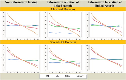
Figure 2. Simulation A with random domain effects: Relative bias (%) of domain mean estimators. Horizontal axis represents the different domains.

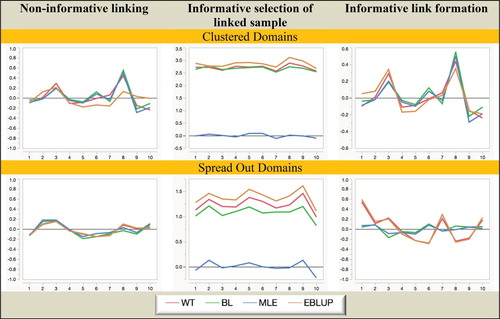
Figure 3. Simulation A with fixed domain effects: Relative RMSE (%) of domain mean estimators. Horizontal axis represents the different domains.

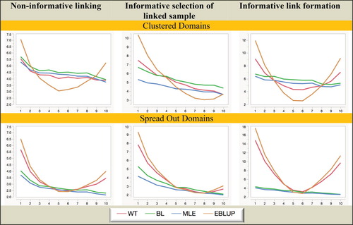
Figure 4. Simulation A with random domain effects: Relative RMSE (%) of domain mean estimators. Horizontal axis represents the different domains.

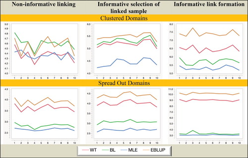
Figure 5. Simulation A with fixed domain effects: Coverage (nominal = 95%) of domain mean estimators. Horizontal axis represents the different domains.

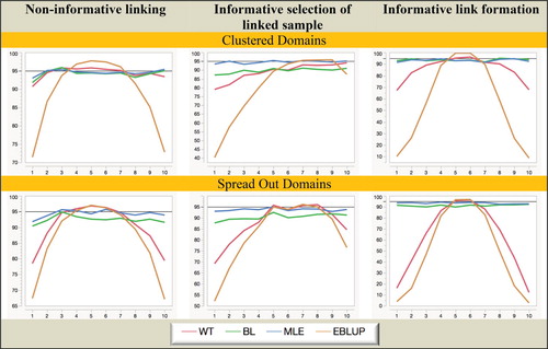
Figure 6. Simulation A with random domain effects: Coverage (nominal = 95%) of domain mean estimators. Horizontal axis represents the different domains.

It is clear from Figures 1 and 2 that MLE is unbiased under all twelve scenarios considered in the study. In contrast, BL is biased when the linked sample is chosen informatively, while both WT and EBLUP are seriously biased when fixed domain effects underpin the response (mainly because of overshrinkage in this case), and are also biased in the random domain effects case when the linked sample is chosen informatively.

When we consider Figures 3 and 4 we see that MLE is still superior to the other three estimators when it comes to MSE efficiency, with BL somewhat less efficient. Surprisingly, EBLUP is almost always the least efficient in random-effects scenarios, while in the fixed effects scenarios it is only efficient where the underlying domain effects are closer to zero. Generally, WT behaves like EBLUP, but tends to be more efficient since it does not shrink as much.

Turning to the coverage performances displayed in Figures 5 and 6, we see that even though no allowance is made for estimation of linkage probabilities (which inflates variance) in variance estimation, MLE still performs consistently well in all scenarios. BL also performs creditably in terms of coverage, but problems with overshrinkage and bias for WT and EBLUP lead to poor coverage in fixed effects scenarios. In random-effects scenarios WT performs slightly better, but EBLUP remains a poor performer.

Overall, from the Simulation A results set out in Figures 1–6 we see that informative choice of which linked records to use in analysis is problematic for all estimators except MLE, while informative linkage error leads to the largest inefficiencies for WT and EBLUP. That is, MLE (which assumes linkage error follows a noninformative ELE model and a fixed effect specification for the domains of interest) seems to be generally robust to the two different types of informative linkage we consider in this paper. It also seems to be robust to a fixed versus random effects specification for the response.

However, Simulation A can be criticised because it assumes reasonably large sample sizes (average of 20 per domain) and a small number (10) of domains. It may well be that some of the robust performance of MLE noted above was a consequence of this choice. We therefore also report results for an extension of this simulation study, which we refer to as Simulation B. Essentially this extends the situation of interest to more domains (30) and smaller domain samples (average of 10 per domain). In particular, we fix the total sample size at 300, made up of 150, 90 and 60 in each block. No changes are made to any of the other parameters governing the behaviour of the study. We also only show results for random domain effects since these are closer to the underlying small area estimation paradigm. Similar results (not shown) were obtained for fixed domain effects. As in Simulation A, domains are numbered in rank order of their expected values.

Considering the behaviour displayed in Figures 7–9 we see that there are some changes compared with Figures 1–6. Not surprisingly, all estimators demonstrate increased variability. However, BL is also much more unstable under informative linking. This is particularly striking when one looks at the MSE results for BL under informative link formation as shown in Figure 8. The reason for this is not entirely clear at the time of writing. One possibility is that its second-order optimal weights become increasingly unstable given the smaller sample sizes used in this situation. It is tempting in such cases to use simpler weights, for example, the weights implied by the approach of Lahiri and Larsen (2005). However, although we do not present these results here, we also calculated the estimates defined by these alternative weighting regimes in our simulations and observed essentially the same behaviour as reported for BL. It, therefore, seems more likely that the instability of BL under informative linking reflects an inherent issue with a purely sampled-based weighting approach in this situation rather than any particular choice of weights.

Figure 7. Simulation B with random domain effects: Relative Bias (%) of domain mean estimators. Horizontal axis represents the different domains.

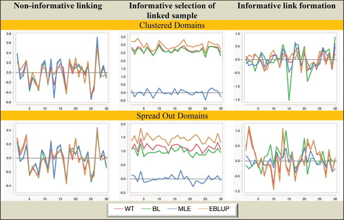
Figure 8. Simulation B with random domain effects: Relative RMSE (%) of domain mean estimators. Horizontal axis represents the different domains.

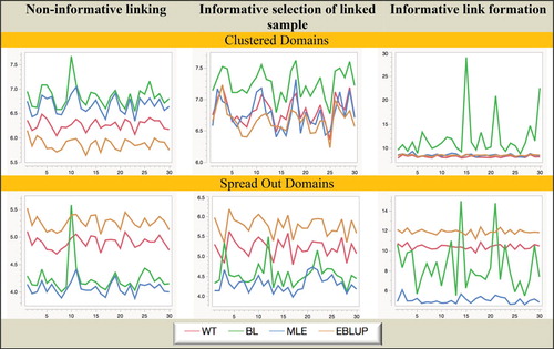
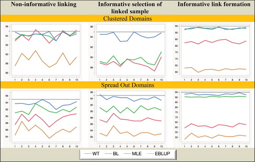
Figure 9. Simulation B with random domain effects: Coverage (nominal = 95%) of domain mean estimators. Horizontal axis represents the different domains.

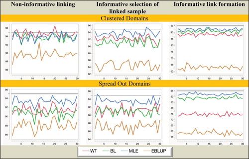
In contrast, MLE remains robust and efficient, even when domain sample sizes are small. In particular, it is the only estimation method that remains unbiased under informative selection of the linked sample. We also note that though generally the EBLUP is still not a good performer in Simulation B, it does demonstrate the best MSE performance under non-informative linkage for the case where the domain means are randomly distributed but also relatively close to each other. This is not unexpected since it is the type of situation where shrinkage can significantly reduce variability. However, when domain means are more spread out, this advantage disappears and WT performs better than EBLUP. Finally, in Figure 9 we see that although all four estimators do not achieve their nominal coverage levels uniformly across the domains, MLE is clearly the best performer overall, while EBLUP is the worst. Since EBLUP demonstrates substantial undercoverage irrespective of whether the linkage is informative or not, it seems most likely the PR MSE estimator used with EBLUP is non-robust to linkage errors.

5. A more realistic linkage exercise

In this section, we provide some illustrative results taken from a much larger study that looked at record linkage of economic data from two registers containing information on 1,280 Brazilian agricultural producers in four states and from four industries followed by estimation of average values of production for each of these four industries. For a more detailed description at this study and the linking methods used in it we refer to Chambers and Diniz da Silva (2019). Here we focus on the performances of two representative record linkage methods that were considered in this study under two different levels of linkage error and the consequent impact on the performances of three of the four estimation methods discussed in the previous section. Note that in what follows states correspond to blocks and industries to domains of interest.

The two record linkage methods are the widely used comparison weights method first introduced in Fellegi and Sunter (1969) and a more recently proposed bootstrapped classification tree-based method based on the Bagging idea developed in Breiman (1994; 1998). Both linkage methods were modified so that they resulted in one to one and complete linkage. Furthermore, since unique identifiers were available in the two registers, as well as names for the different producers, two levels of linking error were evaluated. The first was defined by the errors in the linking variables originally used and was mainly due to errors in the name linking fields. This is denoted as level one error below. The second was more serious and was generated by switching first and second names of producers. This is denoted as level two error below. A total of 200 independent repetitions of linking followed by estimation was next carried out by random sampling with replacement from the available linking variables, including producer name fields containing either level one or level two errors, and then linking the two registers. Table 1 shows summary measures of the linking performance that was achieved over these 200 repetitions for each level of error and for each method of linking. It can be seen that under level one errors there is almost nothing to choose between the linking performances of both linking methods. However, when the extent of the measurement error in the linking variables is increased (level two error), then classification tree-based linkage performs substantially better than comparison weights-based linkage.

Table 1. Summary measures of quality of record linkage for linked Brazilian data.

	Comparison weights (FS) linkage		Classification tree (Bagging) linkage
Averages of linkage quality metrics	Error level 1	Error level 2	Error level 1	Error level 2
Average counts for all pairwise comparisons
True links made	1220	807	1250	1211
False links ignored	634,114	632,701	633,105	634,664
True links ignored	1334	1748	1308	1354
False links made	60	473	30	69

Irrespective of the actual source of the linking errors, ELE linkage errors were next assumed, with blocks corresponding to States. Table 2 shows the average probabilities of correct linkage that were achieved in each block. Note that for comparison weights-based linking the actual linkage error probabilities (not shown here) were observed to vary substantially between domains within some blocks, so the ELE model is in fact, a misspecified LEM for this case. In particular, this indicated the presence of within-block heterogeneity in the linkage error probabilities, and therefore a potentially informative linkage situation. Again, we see that comparison weights-based linkage is substantially impacted by moving from level one to level two errors, while classification tree-based linkage is much less affected.

Table 2. Average probabilities of correct linkage by linkage method and level of error (Block = State) for linked Brazilian data.

	Comparison weights (FS) linkage		Classification tree (Bagging) linkage
Probability of correct linkage	Error level 1	Error level 2	Error level 1	Error level 2
Block 1	0.95	0.74	0.97	0.95
Block 2	0.95	0.52	0.97	0.93
Block 3	1.00	0.92	1.00	1.00
Block 4	0.95	0.72	0.98	0.97

Linked sample data were finally simulated by taking a 10 per cent simple random sample without replacement from the linked registers created by the two linking methods under the two levels of linking error. For each sample, we then computed the industry-level estimates generated by WT, BL and MLE. Note that since all sample weights are the same, WT in this case is just the linked sample mean of value of production in each industry. Since correctly linked register information is available, these estimates could then be evaluated. Table 3 shows bias, MSE and coverage results for nominal 95% Gaussian confidence intervals for industry means.

Table 3. Summary statistics for industry estimates of production using sample-to-register linkage and selected estimators for Brazilian linked data.

	Comparison weights (FS) linkage						Classification tree (Bagging) linkage
	Error level 1			Error level 2			Error level 1			Error level 2
Industry	WT	BL	MLE	WT	BL	MLE	WT	BL	MLE	WT	BL	MLE
	Relative Bias (%)
Crops	−0.04	0.23	0.14	−1.69	0.64	0.33	−0.10	0.03	0.14	−0.18	0.14	0.04
Livestock	0.13	0.26	0.14	−0.83	0.51	0.21	−0.21	−0.15	−0.12	0.05	0.22	0.02
Forestry	−0.05	0.16	−0.14	−0.73	0.32	−0.27	−0.04	0.06	0.00	−0.06	0.13	−0.03
Fishery	0.25	−0.35	−0.36	5.23	−0.30	−0.67	0.11	−0.21	−0.05	0.61	−0.13	−0.09
	Relative RMSE (%)
Crops	1.66	1.74	1.39	2.51	2.78	2.38	1.58	1.59	1.32	1.84	1.91	1.51
Livestock	2.14	2.24	1.52	2.25	3.20	1.89	2.21	2.24	1.46	2.17	2.25	1.45
Forestry	1.30	1.35	1.27	2.00	2.40	1.43	1.46	1.50	1.16	1.42	1.47	1.24
Fishery	1.75	1.84	1.75	5.81	3.96	2.74	1.63	1.67	1.52	2.03	2.06	1.76
	Coverage (%) of nominal 95% Gaussian confidence intervals
Crops	98.0	96.0	96.0	88.4	77.4	94.5	99.0	97.5	98.0	94.0	92.0	95.5
Livestock	86.0	85.0	92.0	93.2	67.8	90.4	90.5	87.5	94.0	88.0	86.0	92.0
Forestry	100.0	100.0	97.0	100.0	84.9	97.3	100.0	100.0	98.5	100.0	100.0	97.5
Fishery	99.5	100.0	98.5	54.8	91.1	96.6	99.5	100.0	97.5	99.0	98.0	97.0

The results set out in Table 3 show that irrespective of the method of linking, or the underlying level of linkage error, MLE is always more efficient, or as efficient, as WT or BL in all four industries. Furthermore, under comparison weights-based linkage and level two linkage errors, WT displays considerably more bias than MLE and BL. Finally, it can be noted that MLE produces confidence intervals for industry means that have coverage performances that are generally much closer to their nominal level of 95%.

6. A summary and some tentative conclusions

With the continued growth in the use of non-deterministic linkage to create data sets for statistical analysis, the impact of linkage errors on this analysis is now an important issue, particularly since this type of measurement error leads to biased inference. Methods for correcting this bias have been proposed, but they typically assume non-informative linkage errors, that is they assume conditional independence of linkage errors and model errors given model covariates. This assumption is not necessarily a safe one, though, since popular third-party linkage procedures cannot guarantee that decisions concerning which records to link (including which linked records to provide the user), or the probabilities of correct linkage themselves, do not themselves depend on characteristics that are correlated with the study variable.

In this paper, we have used simulation to explore the sensitivity to informativeness of linkage errors of two methods for linked data inference, both of which assume non-informative linkage. The two methods are a bias-corrected estimating equation method and maximum likelihood method based on a Gaussian approximation, and we have focussed on domain mean estimation since this is a popular use for linked data. Our results are fairly clear. The maximum likelihood approach shows impressive stability and efficiency under both informative linkage error scenarios that we explored, while the estimating equation approach is somewhat less stable and less efficient. However, it is still preferable to analysis that ignores linkage error in cases where domain sample sizes are not too small. In contrast, standard methods of domain analysis, whether they assume fixed or random domain effects, should be used with considerable caution when the underlying data are probability linked since they can be badly biased if potential linkage errors are informative. This is particularly true when domain effects are assumed to be random, and standard EBLUP-based inference is used. This includes the use of MSE estimation methods for random effects predictors that are known to work well when there is no measurement error but then appear to run into considerable problems when linkage errors are present.

A major issue that we have not attempted to address in this paper is to dig deeper and find out exactly why the Gaussian approximation-based MLE approach does so well under the informative linkage scenarios that we investigated. Even though this approach makes use of ‘calibrating’ block-level information, this type of robustness was not expected a priori. It may be a consequence of this approach relying on second-order assumptions that themselves depend on the one to one and complete linkage assumptions and the simplicity of the ELE structure for linkage errors which, provided blocks are in fact properly identified, can approximate within block informative linkage reasonably well. It is an area that will benefit further investigation, as will extension of the MLE methodology to more complex data and models.

Disclosure statement

No potential conflict of interest was reported by the authors.

ORCID

Nicola Salvati http://orcid.org/0000-0002-4160-9387

Enrico Fabrizi http://orcid.org/0000-0003-2504-7043

Additional information

Notes on contributors

Ray Chambers

Ray Chambers is Honorary Professorial Fellow at the National Institute for Applied Statistics Research Australia. His research is focused on robust model–based methods for inference from complex data, and particularly where this complexity arises through integration of data from multiple sources.

Nicola Salvati

Nicola Salvati is associate professor in Statistics at the University of Pisa, Pisa, Italy. He holds a PhD in Applied Statistics from the Department of Statistics ‘G. Parenti’, University of Florence. His research interests cover robust statistics, small area estimation, survey sampling methodology, quantile and M-quantile regression, multilevel models and spatial statistics.

Enrico Fabrizi

Enrico Fabrizi is associate professor in Statistics at the University Cattolica del Sacro Cuore (Catholic University of the Sacred Heart), Milan, Italy. He holds a PhD in Statistics from the Department of Statistics, University of Bologna. His research interests cover survey sampling methodology, Bayesian inference applied to the analysis of complex survey data and small area estimation.

Andrea Diniz da Silva

Andrea Diniz da Silva is a Professor in the National School of Statistical Science, Rio de Janeiro, Brazil and holds a PhD in Public Statistics from the same institution. She is also a senior statistician in the Methodology Department of the Brazilian Institute of Geography and Statistics.

References

- Breiman, L. (1994). Bagging predictors (Technical Report No. 421). Berkeley: Department of Statistics University of California.
- Breiman, L. (1998). Arcing classifiers. The Annals of Statistics, 26, 801-849. doi: 10.1214/aos/1024691079
- Chambers, R. (2009). Regression analysis of probability-linked data. Statisphere, Official Statistics Research Series, Volume 4.
- Chambers, R., & Diniz da Silva, A. (2019). Improved secondary analysis of linked data. To Appear in Journal of the Royal Statistical Society Series A. doi:10.1111/rssa.12477.
- Fellegi, I. P., & Sunter, A. B. (1969). A theory for record linkage. Journal of the American Statistical Association, 64, 1183–1210. doi: 10.1080/01621459.1969.10501049
- Kim, G., & Chambers, R. (2012). Regression analysis under incomplete linkage. Computational Statistics and Data Analysis, 56, 2756–2770. doi: 10.1016/j.csda.2012.02.026
- Lahiri, P., & Larsen, M. D. (2005). Regression analysis with linked data. Journal of the American Statistical Association, 100, 222–230. doi: 10.1198/016214504000001277
- Prasad, N. G. N., & Rao, J. N. K. (1990). The estimation of the mean squared error of small-area estimators. Journal of the American Statistical Association, 85, 163–171. doi: 10.1080/01621459.1990.10475320