Convergence rate of principal component analysis with local-linear smoother for functional data under a unified weighing scheme

ABSTRACT

The unified weighing scheme for the local-linear smoother in analysing functional data can deal with data that are dense, sparse or of neither type. In this paper, we focus on the convergence rate of functional principal component analysis using this method. Almost sure asymptotic consistency and rates of convergence for the estimators of eigenvalues and eigenfunctions have been established. We also provide the convergence rate of the variance estimation of the measurement error. Based on the results, the number of observations within each curve can be of any rate relative to the sample size, which is consistent with the earlier conclusions about the asymptotic properties of the mean and covariance estimators.

KEYWORDS:

• Functional principal components
• asymptotic properties
• local-linear smoothing
• weighing scheme

1. Introduction

In this article, we consider the typical functional data setting, where a sample of n curves are observed over the time range $\mathcal{T}$, each at $m_i$ discrete points for $i=1,\dots ,n$. When analysing such data, sparsity of the time grid at which the measurements are observed should be taken into account, and proper estimation procedures would be adopted accordingly. Conventionally, pre-smoothing the observations from each subject is viable for dense data before subsequent ?>analysis, whereas the subjects are pooled to borrow information for sparse data; furthermore, two types of estimation procedures present different asymptotic properties (Zhang & Wang, 2016). For the essential problem of estimating the mean and covariance functions, we refer to, for example, Ferraty and Vieu (2006), Ramsay and Silverman (2005), Rice and Silverman (1991), Staniswalis and Lee (1998), Zhou, Lin, and Liang (2017) and references therein.

Here we focus on local-linear smoother, which has high popularity due to its conceptual simplicity, attractive local features and ability for automatic boundary correction (Fan & Gijbels, 1996). To ensure that the effect of each curve on the optimisers is not overly affected by the denseness of observations, different weighing schemes have been proposed. A scatter plot smoother is employed by Yao, Müller, and Wang (2005), which assigns the same weight to each observation for sparse functional data analysis, referred to as the ‘OBS’ scheme. Alternatively, Li and Hsing (2010) suggested a unified framework in which the number of observations within each curve can be of any rate relative to the sample size, where each subject received the same weight, referred to as the ‘SUBJ’ scheme. More recently, Zhang and Wang (2016) proposed a more general weighing scheme which includes the previous two commonly used schemes as special cases, and provided a comprehensive and unifying analysis of the asymptotic properties for estimation.

In addition to the essential estimation problem, functional principal component analysis (FPCA) has become a common part in functional data analysis, for example, to achieve dimension reduction of functional data by summarising the data in a few functional principal component (FPC) scores, or to interpret the varying trend of individual trajectories with the eigenfunctions. For a comprehensive discussion on FPCA, one may refer to Greven, Crainiceanu, Caffo, and Reich (2010), Hall, Müller, and Wang (2006), James, Hastie, and Sugar (2000), Jiang and Wang (2010), Yao and Lee (2006), and the references therein. Although there has been a lot of literature on FPCA, only a few theoretical studies on FPCA have been made, such as in Hall and Hosseini-Nasab (2006), Hall et al. (2006) and Li and Hsing (2010), and they are all based on ‘OBS’ or ‘SUBJ’ scheme. The convergence rates of the eigenvalues and eigenfunctions for the FPCA have not been studied under the general weighing scheme. The theoretical results in the paper not only provide the upper bounds of the convergence rates of eigenvalues and eigenfunctions under a unified weighing scheme but also provide bases for further theoretical studies on functional clustering and classification based on the FPCA method.

The work of Zhang and Wang (2016) established the asymptotic normality, $L^2$ convergence, and uniform convergence for the mean and covariance estimators, but not the asymptotic properties of the FPC. Under the general weighing scheme, we provide in this article the almost sure convergence rate for eigenvalues and eigenfunctions, and further the convergence rate for the variance estimation of the measurement errors. The rest of the article is organised as follows. Notations, model and methodology including FPCA are included in Section 2. The main results about convergence rate in eigenvalues, eigenfunctions and the variance estimation of measurement errors are established in Section 3, with all technical proofs left to the Appendix. Simulation studies to verify the theoretical results are shown in Section 4. The concluding remarks are given in Section 5.

2. Model and methodology

Consider a random process $X\left(t\right)$ defined on a fixed interval $\mathcal{T}=[0,1]$ with mean function $\mu \left(t\right)=E\left\{X\right(t\left)\right\}$ and covariance function $\gamma (s,t)=\mathrm{c}\mathrm{o}\mathrm{v}\left\{X\right(s),X(t\left)\right\}$. Denote with $Y_{ij}$ the error-prone observations of the random process at random points $T_{ij}$, that is $Y_{ij}=X_i\left(T_{ij}\right)+{\epsilon }_{ij},i=1,\dots ,n,j=1,\dots ,m_i;$ where the $X_i$s are realisations of X, ${\epsilon }_{ij}={\epsilon }_i\left(t_{ij}\right)$ are identically distributed measurement errors with mean zero and variance ${\sigma }^2$, and all the $X_i$s, $T_{ij}$s and ${\epsilon }_{ij}$s are assumed to be independent.

2.1. Local-linear smoother

A local-linear estimator of the mean function $\hat{\mu }\left(t\right)={\hat{\beta }}_0$ is obtained by minimising the weighted least squares $\sum _{i=1}^n{\omega }_i\sum _{j=1}^{m_i}{K}_{h_1}\left(T_{ij}-t\right){\left\{Y_{ij}-{\beta }_0-{\beta }_1(T_{ij}-t)\right\}}^2,$ with respect to $({\beta }_0,{\beta }_1)$, where $K_h(\cdot )=h^{-1}K(\cdot /h)$ is a kernel with bandwidth h. It was proposed in Zhang and Wang (2016) to assign weight ${\omega }_i$ to each observation for the ith subject such that $\sum _{i=1}^n{m}_i{\omega }_i=1$, which is the general weighing scheme. Specifically, assignment ${\omega }_i=1/\sum _{i=1}^n{m}_i$ along with ${\nu }_i=1/\sum _{i=1}^n{m}_i(m_i-1)$ leads to the OBS scheme; assignment ${\omega }_i=1/\left(n{m}_i\right)$ along with ${\nu }_i=1/n{m}_i(m_i-1)$ leads to the SUBJ scheme.

To estimate the covariance function $\gamma (s,t)$, we first estimate $G(s,t)=E\left\{X\right(s\left)X\right(t\left)\right\}$, and then it follows that (1) $\hat{\gamma }(s,t)=\hat{G}(s,t)-\hat{\mu }\left(s\right)\hat{\mu }\left(t\right).$(1) Similarly as before, a local-linear estimator $\hat{G}(s,t)={\hat{\beta }}_0$ is obtained by minimising the weighted least squares $\begin{array}{rl}& \sum _{i=1}^n{\nu }_i\sum _{1\le j\ne l\le m_i}{K}_{h_2}\left(T_{ij}-s\right)K_{h_2}\left(T_{il}-t\right)\\ & {\left\{Y_{ij}{Y}_{il}-{\beta }_0-{\beta }_{11}(T_{ij}-s)-{\beta }_{12}(T_{il}-t)\right\}}^2,\end{array}$ where weight ${\nu }_i$ is attached to each $Y_{ij}{Y}_{il}$ for the ith subject such that $\sum _{i=1}^n{m}_i(m_i-1){\nu }_i=1$.

Finally to estimate the variance of measurement errors, we start by a local-linear estimator $\hat{V}\left(t\right)={\hat{\beta }}_0$ of $V\left(t\right):=G(t,t)+{\sigma }^2$, obtained by minimising $\sum _{i=1}^n{\omega }_i\sum _{j=1}^{m_i}{K}_{h_3}\left(T_{ij}-t\right)\{Y_{ij}^2-{\beta }_0-{\beta }_1(T_{ij}-t){\}}^2.$ We then estimate ${\sigma }^2$ by ${\hat{\sigma }}^2={\int }_0^1\left\{\hat{V}\right(t)-\hat{G}(t,t\left)\right\}\mathrm{d}t$. Throughout this article, we select the bandwidths $h_1,h_2$ and $h_3$ by using the leave-one-out cross-validation method.

2.2. Functional principal component analysis

We consider a spectral decomposition of $\gamma (s,t)$ and its approximation. According to Mercer's theorem, the covariance function has the spectral decomposition $\gamma (s,t)=\sum _{j=1}^{\mathrm{\infty }}{\lambda }_j{\phi }_j\left(s\right){\phi }_j\left(t\right),$ where ${\lambda }_1\ge {\lambda }_2\ge \cdots \ge 0$ are the eigenvalues of $\gamma (\cdot ,\cdot )$, and the ${\phi }_j^{\prime }$s are the corresponding eigenfunctions, i.e., the principal components, which form an orthonormal system on the space of square-integrable functions on [0,1]. Following the Karhunen–Loève expansion, $X_i\left(t\right)$ is represented as $X_i\left(t\right)=\mu \left(t\right)+\sum _{j=1}^{\mathrm{\infty }}{\xi }_{ij}{\phi }_j\left(t\right)$, where ${\xi }_{ij}={\int }_0^1{X}_i\left(t\right){\phi }_j\left(t\right)\mathrm{d}t$ is referred to as the jth FPC score of the ith subject. For each i, the ${\xi }_{ij}$ s are uncorrelated random variables with $E\left({\xi }_{ij}\right)=0$ and $E\left({\xi }_{ij}^2\right)={\lambda }_j$.

With the local-linear estimate $\hat{\gamma }(s,t)$, we can approximate it with $\hat{\gamma }(s,t)=\sum _{j=1}^K{\hat{\lambda }}_j{\hat{\phi }}_j\left(s\right){\hat{\phi }}_j\left(t\right),$ where ${\hat{\lambda }}_1\ge {\hat{\lambda }}_2\ge \cdots \ge 0$ are the estimated eigenvalues, the ${\hat{\phi }}_j$s are the corresponding estimated eigenfunctions, and K is the number of principal components selected. We refer to Hall et al. (2006) and Yao et al. (2005) for comprehensive discussions about computation of the eigenvalues and eigenfunctions of an integral operator with a symmetric kernel. We refer to Li, Wang, and Carroll (2013) for intensive discussions about the choice of K and the underlying theory of the functional principal component analysis.

3. Main results about convergence rates

A few more notations are introduced first. Given a positive integer k, we denote $M_{Sk}=\sum _{i=1}^n{m}_i^k$, $\overline{M}=\sum _{i=1}^n{m}_i/n$, ${\overline{M}}_{Sk}=M_{Sk}/n$ and ${\overline{M}}_{Hk}=(n^{-1}\sum _{i=1}^n{m}_i^{-k}{)}^{-1}$, where the subscript ‘H’ in ${\overline{M}}_H$ suggests a harmonic mean. The asymptotic behaviour of estimated eigenvalues and eigenfunctions is given in Theorem 3.1.

Theorem 3.1

Suppose that the regularity conditions (A1)–(A2), (B1)–(B4), (C1)–(C2) and (D1)–(D2) in the Appendix hold. For any fixed j, we have the following results :

1. convergence rate of estimated eigenvalue $\begin{array}{rl}{\hat{\lambda }}_j-{\lambda }_j& =O(\left(\mathrm{l}\mathrm{o}\mathrm{g}\right(n)/n{)}^{1/2}+h_1^2+h_2^2+\mathrm{l}\mathrm{o}\mathrm{g}(n)\\ & [\frac{\sum _{i=1}^n{m}_i{\omega }_i^2}{h_1}+\sum _{i=1}^n{m}_i(m_i-1){\omega }_i^2]\\ & +\mathrm{l}\mathrm{o}\mathrm{g}\left(n\right)[\frac{\sum _{i=1}^n{m}_i(m_i-1){\nu }_i^2}{h_2^2}\\ & +\frac{\sum _{i=1}^n{m}_i(m_i-1)(m_i-2){\nu }_i^2}{h_2}\\ & +\sum _{i=1}^n{m}_i(m_i-1)(m_i-2)(m_i-3){\nu }_i^2])\\ & a.s.\end{array}$

2. convergence rate of estimated eigenfunction $\begin{array}{rl}& \underset{t\in [0,1]}{sup}|{\hat{\phi }}_j\left(t\right)-{\phi }_j\left(t\right)|\\ & =O(h_1^2+\{\mathrm{l}\mathrm{o}\mathrm{g}\left(n\right)[\frac{\sum _{i=1}^n{m}_i{\omega }_i^2}{h_1}\\ & +\sum _{i=1}^n{m}_i(m_i-1){\omega }_i^2]{\}}^{1/2}+h_2^2\\ & +\{\mathrm{l}\mathrm{o}\mathrm{g}\left(n\right)[\frac{\sum _{i=1}^n{m}_i{\omega }_i^2}{h_2}+\sum _{i=1}^n{m}_i(m_i-1){\omega }_i^2]{\}}^{1/2}\\ & +\mathrm{l}\mathrm{o}\mathrm{g}\left(n\right)[\frac{\sum _{i=1}^n{m}_i(m_i-1){\nu }_i^2}{h_2^2}\\ & +\frac{\sum _{i=1}^n{m}_i(m_i-1)(m_i-2){\nu }_i^2}{h_2}\\ & +\sum _{i=1}^n{m}_i(m_i-1)(m_i-2)(m_i-3){\nu }_i^2])a.s.\end{array}$

In the following, we state in Corollary 3.2 and Corollary 3.3 the specialised results for the OBS and SUBJ schemes, respectively. For either the OBS or SUBJ scheme, convergence rate depends on the order of ${\overline{M}}_{Sk}$ and ${\overline{M}}_{Hk}$ relative to n and the order of bandwidth.

Corollary 3.2

Suppose that the conditions in Theorem 3.1 hold, along with two additional assumptions (C3) and (D3). Then under the OBS scheme, for any fixed j,

1. $\begin{array}{rl}{\hat{\lambda }}_j-{\lambda }_j& =O(\left(\mathrm{l}\mathrm{o}\mathrm{g}\right(n)/n{)}^{1/2}+h_1^2+h_2^2\\ & +(\frac{1}{\overline{M}{h}_1}+\frac{{\overline{M}}_{S2}}{(\overline{M}{)}^2})\frac{\mathrm{l}\mathrm{o}\mathrm{g}\left(n\right)}{n}\\ & +(\frac{1}{{\overline{M}}_{S2}{h}_2^2}+\frac{{\overline{M}}_{S3}}{({\overline{M}}_{S2}{)}^2{h}_2}\\ & +\frac{{\overline{M}}_{S4}}{({\overline{M}}_{S2}{)}^2})\frac{\mathrm{l}\mathrm{o}\mathrm{g}\left(n\right)}{n})a.s.\end{array}$

2. $\begin{array}{rl}& \underset{t\in [0,1]}{sup}|{\hat{\phi }}_j\left(t\right)-{\phi }_j\left(t\right)|\\ & =O(h_1^2+\sqrt{(\frac{1}{\overline{M}{h}_1}+\frac{{\overline{M}}_{S2}}{(\overline{M}{)}^2})\frac{\mathrm{l}\mathrm{o}\mathrm{g}\left(n\right)}{n}}+h_2^2\\ & +\sqrt{(\frac{1}{\overline{M}{h}_2}+\frac{{\overline{M}}_{S2}}{(\overline{M}{)}^2})\frac{\mathrm{l}\mathrm{o}\mathrm{g}\left(n\right)}{n}}\\ & +(\frac{1}{{\overline{M}}_{S2}{h}_2^2}+\frac{{\overline{M}}_{S3}}{({\overline{M}}_{S2}{)}^2{h}_2}\\ & +\frac{{\overline{M}}_{S4}}{({\overline{M}}_{S2}{)}^2})\frac{\mathrm{l}\mathrm{o}\mathrm{g}\left(n\right)}{n})a.s.\end{array}$

Corollary 3.3

Suppose that the conditions in Theorem 3.1 hold. Then under the SUBJ scheme, for any fixed j,

1. $\begin{array}{rl}& {\hat{\lambda }}_j-{\lambda }_j\\ & =O(\left(\mathrm{l}\mathrm{o}\mathrm{g}\right(n)/n{)}^{1/2}+h_1^2+h_2^2\\ & +(\frac{1}{{\overline{M}}_H{h}_1}+1)\frac{\mathrm{l}\mathrm{o}\mathrm{g}\left(n\right)}{n}\\ & +(\frac{1}{{\overline{M}}_{H2}{h}_2^2}+\frac{1}{{\overline{M}}_H{h}_2}+1)\frac{\mathrm{l}\mathrm{o}\mathrm{g}\left(n\right)}{n})a.s.\end{array}$

2. $\begin{array}{rl}& \underset{t\in [0,1]}{sup}|{\hat{\phi }}_j\left(t\right)-{\phi }_j\left(t\right)|\\ & =O(h_1^2+\sqrt{(\frac{1}{{\overline{M}}_H{h}_1}+1)\frac{\mathrm{l}\mathrm{o}\mathrm{g}\left(n\right)}{n}}+h_2^2\\ & +\sqrt{(\frac{1}{{\overline{M}}_H{h}_2}+1)\frac{\mathrm{l}\mathrm{o}\mathrm{g}\left(n\right)}{n}}\\ & +(\frac{1}{{\overline{M}}_{H2}{h}_2^2}+\frac{1}{{\overline{M}}_H{h}_2}+1)\frac{\mathrm{l}\mathrm{o}\mathrm{g}\left(n\right)}{n})a.s.\end{array}$

In addition, we provide below the convergence rate of the estimated variance of the measurement error under the general weighing scheme, as well as the special cases of the OBS and SUBJ schemes.

Theorem 3.4

Assume that the conditions in Theorem 3.1, and conditions (C1') and (C2') hold. Then under the general weighing framework, $\begin{array}{rl}& {\hat{\sigma }}^2-{\sigma }^2\\ & =O(h_2^2+\{\mathrm{l}\mathrm{o}\mathrm{g}\left(n\right)[\frac{\sum _{i=1}^n{m}_i{\omega }_i^2}{h_1}\\ & +\sum _{i=1}^n{m}_i(m_i-1){\omega }_i^2]{\}}^{1/2}\\ & +\mathrm{l}\mathrm{o}\mathrm{g}\left(n\right)[\frac{\sum _{i=1}^n{m}_i(m_i-1){\nu }_i^2}{h_2^2}\\ & +\frac{\sum _{i=1}^n{m}_i(m_i-1)(m_i-2){\nu }_i^2}{h_2}\\ & +\sum _{i=1}^n{m}_i(m_i-1)(m_i-2)(m_i-3){\nu }_i^2]\\ & +h_3^2+\mathrm{l}\mathrm{o}\mathrm{g}\left(n\right)[\frac{\sum _{i=1}^n{m}_i{\omega }_i^2}{h_3}\\ & +\sum _{i=1}^n{m}_i(m_i-1){\omega }_i^2])a.s.\end{array}$

Corollary 3.5

Suppose that the conditions in Theorem 3.4 hold.

1. OBS: With an additional assumption (C3), $\begin{array}{rl}& {\hat{\sigma }}^2-{\sigma }^2\\ & =O(h_2^2+\sqrt{(\frac{1}{\overline{M}{h}_2}+\frac{{\overline{M}}_{S2}}{(\overline{M}{)}^2})\frac{\mathrm{l}\mathrm{o}\mathrm{g}\left(n\right)}{n}}\\ & +(\frac{1}{{\overline{M}}_{S2}{h}_2^2}+\frac{{\overline{M}}_{S3}}{({\overline{M}}_{S2}{)}^2{h}_2}+\frac{{\overline{M}}_{S4}}{({\overline{M}}_{S2}{)}^2})\frac{\mathrm{l}\mathrm{o}\mathrm{g}\left(n\right)}{n}\\ & +h_3^2+(\frac{1}{\overline{M}{h}_3}+\frac{{\overline{M}}_{S2}}{(\overline{M}{)}^2})\frac{\mathrm{l}\mathrm{o}\mathrm{g}\left(n\right)}{n})a.s.\end{array}$

2. SUBJ: $\begin{array}{rl}& {\hat{\sigma }}^2-{\sigma }^2\\ & =O(h_2^2+\sqrt{(\frac{1}{{\overline{M}}_H{h}_2}+1)\frac{\mathrm{l}\mathrm{o}\mathrm{g}\left(n\right)}{n}}\\ & +(\frac{1}{{\overline{M}}_{H2}{h}_2^2}+\frac{1}{{\overline{M}}_H{h}_2}+1)\frac{\mathrm{l}\mathrm{o}\mathrm{g}\left(n\right)}{n}+h_3^2\\ & +(\frac{1}{{\overline{M}}_H{h}_3}+1)\frac{\mathrm{l}\mathrm{o}\mathrm{g}\left(n\right)}{n}).\end{array}$

4. Simulation

To illustrate the theoretical results in Section 2, we now turn to the numerical performance of the estimators as sample size increases. Choices on ${\omega }_i$ and ${\nu }_i$ that satisfy the conditions in the general weighing scheme must be made. Since the ‘OBS’ and ‘SUBJ’ cases are the two most commonly used choices, and our corollaries showed the specific results regarding these two cases, we use these two cases as examples to illustrate the theoretical results. The data are generated from the following model: $Y_{ij}=X_i\left(T_{ij}\right)+{\epsilon }_{ij},$ where $X_i\left(t\right)=\mu \left(t\right)+\sum _{k=1}^2{\xi }_{ik}{\phi }_k\left(t\right)$, ${\xi }_{ik}\sim N(0,{\lambda }_k)$ for k = 1, 2 and ${\epsilon }_{ij}\sim N(0,{\sigma }^2)$. Let $\mu \left(t\right)=t+\sin \left(t\right)+\cos \left(t\right)$, ${\phi }_1\left(t\right)=-\sqrt{2}\cos \left(\pi t\right)$, ${\phi }_2\left(t\right)=\sqrt{2}\sin \left(\pi t\right)$, set $({\lambda }_1,{\lambda }_2,{\sigma }^2)=(0.6,0.3,0.2)$.

The observation times are generated in the following way. Each individual has a set of ‘scheduled’ time points, $\{1,2,\dots ,20\}$, and each scheduled time has a 20% probability of being skipped. The actual observation time is a random perturbation of a scheduled time: a uniform [0,1] random variable is added to a nonskipped scheduled time. This results in different observed time points $T_{ij}$ per subject.

To illustrate that the convergence rates of the estimated ${\hat{\lambda }}_k$, ${\hat{\phi }}_k$ and ${\hat{\sigma }}^2$ have the orders of magnitude shown in Section 2, let ${\delta }_{{\lambda }_k}=({\hat{\lambda }}_k-{\lambda }_k)/a_n$, where $a_n$ is the derived convergence rate (e.g., under the OBS scheme, $a_n=\left(\mathrm{l}\mathrm{o}\mathrm{g}\right(n)/n{)}^{1/2}+h_1^2+h_2^2+\left(\frac{1}{\overline{M}{h}_1}+\frac{{\overline{M}}_{S2}}{(\overline{M}{)}^2}\right)\frac{\mathrm{l}\mathrm{o}\mathrm{g}\left(n\right)}{n}+\left(\frac{1}{{\overline{M}}_{S2}{h}_2^2}+\frac{{\overline{M}}_{S3}}{({\overline{M}}_{S2}{)}^2{h}_2}+\frac{{\overline{M}}_{S4}}{({\overline{M}}_{S2}{)}^2}\right)\frac{\mathrm{l}\mathrm{o}\mathrm{g}\left(n\right)}{n}$), if the estimated ${\hat{\lambda }}_k$ is actually consistent with ${\lambda }_k$ by this order of magnitude, the range of the term ${\delta }_{{\lambda }_k}$ should decrease or remain constant as n increases. Here we set n = 50, 75, 100, 125, 150, 175, 200 for both ‘OBS’ and ‘SUBJ’ cases, and 200 replications were done for each sample size.

The procedure is visualised in Figures 1–3. The number of K in each replication was chosen by the 90% fraction of explained variance. As shown in Figure 1, the ranges (under ‘OBS’ scheme) for ${\delta }_{{\lambda }_k}$ (top two panels) and ${\delta }_{{\phi }_k\left(t\right)}$ (bottom two panels) for k = 1, 2 tend to be stable or go down, as the sample size n increases. This demonstrates that the derived order of magnitude of convergence rate in Corollary 3.2 is reasonable.

Figure 1. This is for the ‘OBS’ case. The top two panels present the values of ${\delta }_{{\lambda }_1}$ and ${\delta }_{{\lambda }_2}$ for 200 replications as n increases, respectively. The bottom two panels present the values of ${\delta }_{{\phi }_1\left(t\right)}$ and ${\delta }_{{\phi }_2\left(t\right)}$ for 200 replications as n increases, respectively.

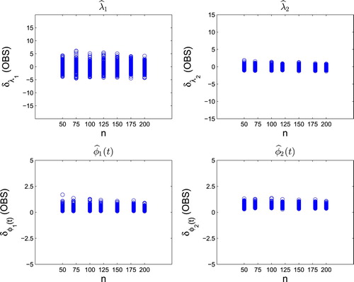
Figure 2. This is for the ‘SUBJ’ case. The top two panels present the values of ${\delta }_{{\lambda }_1}$ and ${\delta }_{{\lambda }_2}$ for 200 replications as n increases, respectively. The bottom two panels present the values of ${\delta }_{{\phi }_1\left(t\right)}$ and ${\delta }_{{\phi }_2\left(t\right)}$ for 200 replications as n increases, respectively.

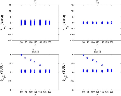
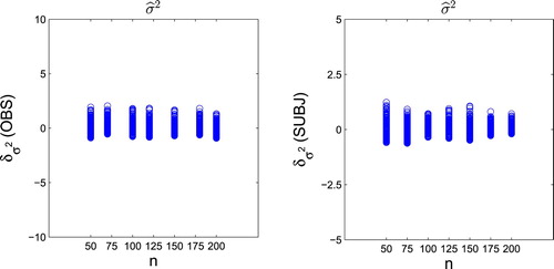
Figure 3. Plots of ${\delta }_{{\sigma }^2}$ for ‘OBS’ (the left panel) and ‘SUBJ’ (the right panel), respectively.

A similar phenomenon under the ‘SUBJ’ scheme can be observed in Figure 2, which shows the converging processes of the estimators ${\hat{\lambda }}_k$ and ${\hat{\phi }}_k$ for k = 1, 2. Although there are some abnormal values in the estimates of eigenfunctions (shown in the left bottom and right bottom panel), generally the fluctuation range tends to be stable. And as expected, the abnormal values disappear as the sample size increases. This shows that the derived convergence rates in Corollary 3.3 is reasonable.

Furthermore, the ${\delta }_{{\sigma }^2}$ under the ‘OBS’ and ‘SUBJ; schemes are plotted in Figure 3. Observe that as the sample size increases, the range of variation of the 200 replications tends to be stable, which demonstrates the results of Corollary 3.5.

5. Discussion

It is common in functional data analysis literature that a method focuses on either dense or sparse data, while discussions about data of neither type are much less. Due to different behaviours of the two types of methods, one needs to choose properly the analysis method when dealing with real data, which is not necessarily as easy as it looks like. For example, we may face a mixture of densely and sparsely observed curves, or even it may be difficult to decide a sampling density. In this sense, methods that can handle any type of data are appreciated. And the method we consider in this article belongs to this category. Specifically, we investigate the almost sure convergence of functional principal component analysis following Zhang and Wang (2016) and complement the unified theoretical framework they set up. We also note that the special case of Corollary 3.3 under SUBJ scheme is consistent with Theorem 3.6 in Li and hsing (2010). The convergence rate of Corollary 3.2 under OBS scheme is better than that of Corollary 1 in Yao et al. (2005), due to different techniques of proofs. We prove with asymptotic expansions of the eigenvalues and eigenfunctions of estimated covariance function (Hall and Hosseini-Nasab (2006) and Hall et al. (2006)) and strong uniform convergence rate of $\hat{\gamma }(s,t)$ by Lemma 5.1 in this article, which lead to a better convergence rate. It is also of great interest to establish the asymptotic distribution and optimal convergence rate of ${\hat{\phi }}_j\left(t\right)$ under the general weighing framework, which we left for future work. Furthermore, the general weighing framework may be used in functional data regression, classification, clustering, etc., and hence the theoretical results here could be extended to those cases as well. This will also be pursued as future work.

Disclosure statement

No potential conflict of interest was reported by the authors.

Additional information

Funding

The work was supported by National Natural Science Foundation of China (project number: 11771146, 11831008, 81530086, 11771145), the National Social Science Foundation Key Program (17ZDA091), the 111 Project (B14019) and Program of Shanghai Subject Chief Scientist (14XD1401600). This work was also supported by the China Postdoctoral Science Foundation (2018M630393). We thank Professors Yanyuan Ma and Yukun Liu for very helpful discussions.

Notes on contributors

Xingyu Yan

Xingyu Yan is currently a Ph.D. candidate in the School of Statistics at East China Normal University. He is interested in functional data analysis.

Xiaolong Pu

Xiaolong Pu is currently Professor of statistics in the School of Statistics at East China Normal University. He is interested in applied statistics, particularly in statistical testing via sampling, statistical process control, sequential analysis and reliability. He received a Ph.D. in Statistics from East China Normal University.

Yingchun Zhou

Yingchun Zhou is currently Professor of statistics in the School of Statistics at East China Normal University. She is interested in functional data analysis and biostatistics. She received a Ph.D. in Statistics from Boston University and worked as a postdoc at National Institute of Statistical Sciences before moving to East China Normal University.

Xiaolei Xun

Xiaolei Xun is currently holding a visiting position in the School of Data Science at Fudan University. She is interested in functional data analysis, Bayesian methods, modeling of high-dimensional data and biostatistics. She received a Ph.D. in Statistics from Texas A&M University and worked in Novartis for five years as biometrician and statistical methodologist before moving to Fudan University.

Appendix

The following regularity conditions that are used to establish the asymptotic properties of the proposed estimators are imposed mainly for mathematical simplicity and may be modified as necessary. In the following, $h_1$, $h_2$ and $h_3$ are bandwidths used in estimating $\mu \left(t\right)$, $\gamma (s,t)$ and $V\left(t\right)$, respectively.

A.1. Regularity conditions

Kernel function

(A1) $K(\cdot )$ is a symmetric probability density function on $[-1,1]$ and ${\sigma }_K^2=\int u^{2}K\left(u\right)du<\mathrm{\infty },{\parallel K\parallel }^2=\int {K\left(u\right)}^2\mathrm{d}u<\mathrm{\infty }.$ (A2) $K(\cdot )$ is Lipschitz continuous: There exists $0<L<\mathrm{\infty }$ such that $|K\left(u\right)-K\left(v\right)|\le L|u-v|,\mathrm{f}\mathrm{o}\mathrm{r}\mathrm{a}\mathrm{n}\mathrm{y}u,v\in [0,1].$ This implies $K(\cdot )\le M_K$ for a constant $M_K$.

Time points and true functions

(B1) {$T_{ij}:i=1,\dots ,n,j=1,\dots ,N_i$}, are $i.i.d.$ copies of a random variable T defined on [0,1]. The density $f(\cdot )$ of T is bounded from below and above: $0<m_f\le \underset{t\in [0,1]}{min}f\left(t\right)\le \underset{t\in [0,1]}{max}f\left(t\right)\le M_f<\mathrm{\infty }.$ Furthermore, $f^{\left(2\right)}(\cdot )$, the second derivative of $f(\cdot )$, is bounded.

(B2) X is independent of T and ϵ is independent of T and U.

(B3) ${\mu }^{\left(2\right)}\left(t\right)$, the second derivative of $\mu \left(t\right)$, is bounded on [0,1].

(B4) ${\mathrm{\partial }}^2\gamma (s,t)/\mathrm{\partial }{s}^2$, ${\mathrm{\partial }}^2\gamma (s,t)/\mathrm{\partial }s\mathrm{\partial }t$ and ${\mathrm{\partial }}^2\gamma (s,t)/\mathrm{\partial }{t}^2$ are bounded on $[0,1{]}^2$.

Conditions for mean estimation

(C1) $h_1\to 0$, $\mathrm{l}\mathrm{o}\mathrm{g}\left(n\right)\sum _{i=1}^n{m}_i{\omega }_i^2/h_1\to 0$, $\mathrm{l}\mathrm{o}\mathrm{g}\left(n\right)\sum _{i=1}^n{m}_i(m_i-1){\omega }_i^2\to 0$.

(C1’) $h_3\to 0$, $\mathrm{l}\mathrm{o}\mathrm{g}\left(n\right)\sum _{i=1}^n{m}_i{\omega }_i^2/h_3\to 0$, $\mathrm{l}\mathrm{o}\mathrm{g}\left(n\right)\sum _{i=1}^n{m}_i(m_i-1){\omega }_i^2\to 0$.

(C2) For some $\alpha >2$, $E\underset{t\in [0,1]}{sup}|X\left(t\right){|}^{\alpha }<\mathrm{\infty }$, $E|\epsilon {|}^{\alpha }<\mathrm{\infty }$ and $n[\sum _{i=1}^n{m}_i{\omega }_i^2{h}_1+\sum _{i=1}^n{m}_i(m_i-1){\omega }_i^2{h}_1^2][\frac{\mathrm{l}\mathrm{o}\mathrm{g}\left(n\right)}{n}{]}^{2/\alpha -1}\to 0.$ (C2') For some $\alpha >2$, $E\underset{t\in [0,1]}{sup}|X\left(t\right){|}^{\alpha }<\mathrm{\infty }$, $E|\epsilon {|}^{\alpha }<\mathrm{\infty }$ and $n[\sum _{i=1}^n{m}_i{\omega }_i^2{h}_3+\sum _{i=1}^n{m}_i\left(m_i-1\right){\omega }_i^2{h}_3^2][\frac{\mathrm{l}\mathrm{o}\mathrm{g}\left(n\right)}{n}{]}^{2/\alpha -1}\to 0.$ (C3) $\underset{n}{sup}\left(n\underset{i}{max}{m}_i{\omega }_i\right)\le B<\mathrm{\infty }.$

Conditions for covariance estimation

(D1)$h_2\to 0$, $\mathrm{l}\mathrm{o}\mathrm{g}\left(n\right)\sum _{i=1}^n{m}_i(m_i-1){\nu }_i^2/h_2^2\to 0$, $\mathrm{l}\mathrm{o}\mathrm{g}\left(n\right)\sum _{i=1}^n{m}_i(m_i-1)(m_i-2){\nu }_i^2/h_2\to 0$, $\mathrm{l}\mathrm{o}\mathrm{g}\left(n\right)\sum _{i=1}^n{m}_i(m_i-1)(m_i-2)(m_i-3){\nu }_i^2\to 0$.

(D2) For some $\beta >2$, $E\underset{t\in [0,1]}{sup}|X\left(t\right){|}^{2\beta }<\mathrm{\infty }$, $E|\epsilon {|}^{2\beta }<\mathrm{\infty }$ and $\begin{array}{rl}& n[\sum _{i=1}^n{m}_i(m_i-1){\nu }_i^2{h}_2^2+\sum _{i=1}^n{m}_i(m_i-1)(m_i-2){\nu }_i^2{h}_2^3\\ & +\sum _{i=1}^n{m}_i(m_i-1)(m_i-2)(m_i-3){\nu }_i^2{h}_2^4]\\ & \times [\frac{\mathrm{l}\mathrm{o}\mathrm{g}\left(n\right)}{n}{]}^{2/\beta -1}\to \mathrm{\infty }.\end{array}$ (D3) $\underset{n}{sup}\left(n\underset{i}{max}{m}_i\right(m_i-1\left){\nu }_i\right)\le B^{\prime }<\mathrm{\infty }.$

The above conditions (A1)–(A2) and (B1)–(B4) are commonly used in the literature of the functional data and longitudinal data (see, e.g. Fan Zhang (2000); Zhu, Li, Kong (2012)). Conditions (C1)–(C3) are used to guarantee the consistency of the mean estimators. Conditions (D1)–(D3) are used to guarantee the consistency of the covariance estimators. For the SUBJ estimators, (C3) and (D3) are automatically satisfied, similar versions of (C2) and (D2) were adopted by Li and Hsing (2010). In addition, (C1') and (C2') are used to guarantee the consistency of measurement error variance estimation.

A.2. Proof

To begin, let us give some notations that will be used in the sequel. Denote $\begin{array}{rl}{S}_r& =\sum _{i=1}^n{\omega }_i\sum _{j=1}^{m_i}{K}_{h_1}(T_{ij}-t){\left(\frac{T_{ij}-t}{h_1}\right)}^r,\\ R_r& =\sum _{i=1}^n{\omega }_i\sum _{j=1}^{m_i}{K}_{h_1}(T_{ij}-t){\left(\frac{T_{ij}-t}{h_1}\right)}^r{Y}_{ij},\\ Q_r& =\sum _{i=1}^n{\omega }_i\sum _{j=1}^{m_i}{K}_{h_3}(T_{ij}-t){\left(\frac{T_{ij}-t}{h_3}\right)}^r{Y}_{ij}^2,\end{array}$ where r = 0, 1, 2, and $\begin{array}{rl}{S}_{pq}& =\sum _{i=1}^n{\nu }_i\sum _{1\le j\ne l\le m_i}{K}_{h_2}(T_{ij}-s)K_{h_2}(T_{il}-t)\\ & \times {\left(\frac{T_{ij}-s}{h_2}\right)}^p{\left(\frac{T_{il}-t}{h_2}\right)}^q\end{array}$ and $\begin{array}{rl}{R}_{pq}& =\sum _{i=1}^n{\nu }_i\sum _{1\le j\ne l\le m_i}{K}_{h_2}(T_{ij}-s)K_{h_2}(T_{il}-t)\\ & \times {\left(\frac{T_{ij}-s}{h_2}\right)}^p{\left(\frac{T_{il}-t}{h_2}\right)}^q{Y}_{ij}{Y}_{il}\end{array}$ where for p, q = 0, 1, 2. For any univariate function $\varphi (\cdot )\in [0,1]$ and a bivariate function $\mathrm{\Psi }(\cdot ,\cdot )\in [0,1{]}^2$, define the $L^2$ norm by $\parallel \varphi \parallel =[\int \varphi (t{)}^2\mathrm{d}t{]}^{1/2}$ and the Hilbert–Schmidt norm by $\mathrm{\Psi }=[\int \int \mathrm{\Psi }(s,t{)}^2\mathrm{d}s\mathrm{d}t{]}^{1/2}$. The domains of the integrals [0,1] are omitted unless otherwise specified.

First, we present the convergence rate of $\hat{\gamma }$ obtained in (1(1) $\hat{\gamma }(s,t)=\hat{G}(s,t)-\hat{\mu }\left(s\right)\hat{\mu }\left(t\right).$(1) ).

Lemma A.1

Under the conditions in Appendix A.1, we have $\begin{array}{rl}& \underset{s,t\in [0,1]}{sup}|\hat{\gamma }(s,t)-\gamma (s,t)|\\ & =O(h_1^2+\{\mathrm{l}\mathrm{o}\mathrm{g}\left(n\right)[\frac{\sum _{i=1}^n{m}_i{\omega }_i^2}{h_1}+\sum _{i=1}^n{m}_i\left(m_i-1\right){\omega }_i^2]{\}}^{1/2}\\ & \times h_2^2+\{\mathrm{l}\mathrm{o}\mathrm{g}\left(n\right)[\frac{\sum _{i=1}^n{m}_i(m_i-1){\nu }_i^2}{h_2^2}\\ & +\frac{\sum _{i=1}^n{m}_i(m_i-1)(m_i-2){\nu }_i^2}{h_2}\\ & +\sum _{i=1}^n{m}_i(m_i-1)(m_i-2)(m_i-3){\nu }_i^2]{\}}^{1/2})a.s.\end{array}$

Proof.

From (1(1) $\hat{\gamma }(s,t)=\hat{G}(s,t)-\hat{\mu }\left(s\right)\hat{\mu }\left(t\right).$(1) ), We note that $\begin{array}{rl}& \underset{s,t\in [0,1]}{sup}|\hat{\gamma }(s,t)-\gamma (s,t)|\\ & \le |\hat{G}(s,t)-G(s,t)|+\mu \left(s\right)\underset{t\in [0,1]}{sup}|\hat{\mu }\left(t\right)-\mu \left(t\right)|\\ & +\hat{\mu }\left(t\right)\underset{s\in [0,1]}{sup}|\hat{\mu }\left(s\right)-\mu \left(s\right)|.\end{array}$ By (B3) and Theorem 5.1 in Zhang and Wang (2016), we have $\mu \left(s\right)\underset{t\in [0,1]}{sup}|\hat{\mu }\left(t\right)-\mu \left(t\right)|,\hat{\mu }\left(t\right)\underset{s\in [0,1]}{sup}|\hat{\mu }\left(s\right)-\mu \left(s\right)|=O\left(\right\{\mathrm{l}\mathrm{o}\mathrm{g}\left(n\right)[\frac{\sum _{i=1}^n{m}_i{\omega }_i^2}{h_1}+\sum _{i=1}^n{m}_i(m_i-1\left){\omega }_i^2\right]{\}}^{1/2})a.s.$. Thus the result can be derived from Theorem 5.2 in Zhang and Wang (2016).

The following lemma is similar with Lemma 6 of Li and Hsing (2010) and will be used in our following proof repeatedly. Let Δ be the integral operator with kernel $\hat{\gamma }-\gamma$.

Lemma A.2

For any bounded measurable function φ on [0,1], $\begin{array}{rl}& \underset{t\in [0,1]}{sup}|\left(\mathrm{\Delta }\phi \right)\left(t\right)|\\ & =O(h_1^2+\{\mathrm{l}\mathrm{o}\mathrm{g}\left(n\right)[\frac{\sum _{i=1}^n{m}_i{\omega }_i^2}{h_1}\\ & +\sum _{i=1}^n{m}_i(m_i-1){\omega }_i^2]{\}}^{1/2}\\ & +h_2^2+\{\mathrm{l}\mathrm{o}\mathrm{g}\left(n\right)[\frac{\sum _{i=1}^n{m}_i{\omega }_i^2}{h_2}\\ & +\sum _{i=1}^n{m}_i(m_i-1){\omega }_i^2]{\}}^{1/2}\\ & +\mathrm{l}\mathrm{o}\mathrm{g}\left(n\right)[\frac{\sum _{i=1}^n{m}_i(m_i-1){\nu }_i^2}{h_2^2}\\ & +\frac{\sum _{i=1}^n{m}_i(m_i-1)(m_i-2){\nu }_i^2}{h_2}\\ & +\sum _{i=1}^n{m}_i(m_i-1)(m_i-2)(m_i-3){\nu }_i^2])a.s.\end{array}$

Proof.

By (1(1) $\hat{\gamma }(s,t)=\hat{G}(s,t)-\hat{\mu }\left(s\right)\hat{\mu }\left(t\right).$(1) ), it follows that $\left(\mathrm{\Delta }\phi \right)\left(t\right)=A_{n1}+A_{n2}$, where $A_{n1}=\int (\hat{G}-G)(s,t)\phi \left(s\right)\mathrm{d}s$ and $A_{n2}=\int \left\{\mu \right(s\left)\mu \right(t)-\hat{\mu }(s\left)\hat{\mu }\right(t\left)\right\}\phi \left(s\right)\mathrm{d}s$. With minor derivation, we have $A_{n1}=\int ({\mathcal{A}}_1{R}_{00}^{\ast }-{\mathcal{A}}_2{R}_{10}^{\ast }-{\mathcal{A}}_3{R}_{01}^{\ast }){\mathcal{B}}^{-1}\phi \left(s\right)\mathrm{d}s,$ where ${\mathcal{A}}_1=S_{20}{S}_{02}-S_{11}^2$, ${\mathcal{A}}_2=S_{10}{S}_{02}-S_{01}{S}_{11}$, ${\mathcal{A}}_3=S_{01}{S}_{20}-S_{10}{S}_{11}$, $\mathcal{B}={\mathcal{A}}_1{S}_{00}-{\mathcal{A}}_2{S}_{10}-{\mathcal{A}}_3{S}_{01}$ and $\begin{array}{rl}{R}_{pq}^{\ast }& =R_{pq}-G(s,t)S_{pq}-h_2\mathrm{\partial }G(s,t)/\mathrm{\partial }s{S}_{p+1,q}\\ & -h_2\mathrm{\partial }G(s,t)/\mathrm{\partial }t{S}_{p,q+1}\text{ for }p,q=0,1.\end{array}$ Further, by Taylor's expansion, (A1) $\begin{array}{rl}{R}_{pq}^{\ast }& =\sum _{i=1}^n{\nu }_i\sum _{1\le j\ne l\le m_i}{\left(\frac{T_{ij}-s}{h_2}\right)}^p\\ & \times {\left(\frac{T_{il}-t}{h_2}\right)}^q{K}_{h_2}(T_{ij}-s)K_{h_2}(T_{il}-t)\\ & \times [Y_{ij}{Y}_{il}-G(T_{ij},T_{ij}\left)\right]+O\left(h_2^2\right).\end{array}$(A1) Applying the proof of Theorem 5.2 in Zhang and Wang (2016), we obtain, uniformly in s, t, (A2) $R_{pq}^{\ast }=O(h_2^2+b_n/h_2)a.s.$(A2) With further calculation, (A3) ${\mathcal{A}}_1=f^2\left(s\right)f^2\left(t\right)({\sigma }_K^2{)}^2+O(h_2+b_n/h_2)a.s.$(A3) and (A4) $\mathcal{B}=f^3\left(s\right)f^3\left(t\right)({\sigma }_K^2{)}^2+O(h_2+b_n/h_2)a.s.,$(A4) where $b_n=\left\{\mathrm{l}\mathrm{o}\mathrm{g}\right(n\left)\right[\sum _{i=1}^n{m}_i(m_i-1){\nu }_i^2{h}_2^2+\sum _{i=1}^n{m}_i(m_i-1)(m_i-2){\nu }_i^2{h}_2^3+\sum _{i=1}^n{m}_i(m_i-1)(m_i-2)(m_i-3){\nu }_i^2{h}_2^4]{\}}^{1/2}$.

We focus on $\int {\mathcal{A}}_1{\mathcal{R}}_{00}^{\ast }{\mathcal{B}}^{-1}\phi \left(s\right)\mathrm{d}s$ since the other two terms can be dealt with similarly. Specifically, $\begin{array}{rl}& \int {\mathcal{A}}_1{\mathcal{R}}_{00}^{\ast }{\mathcal{B}}^{-1}\phi \left(s\right)\mathrm{d}s\\ & =\frac{1}{f\left(t\right)}\sum _{i=1}^n{\omega }_i\sum _{1\le j\ne l\le m_i}\{Y_{ij}{Y}_{il}-G(T_{ij},T_{il}\left)\right\}{K}_{h_2}(T_{il}-t)\\ & \times \int K_{h_2}(T_{ij}-s)\phi \left(s\right)f(s{)}^{-1}ds\\ & +O(h_2^2+\mathrm{l}\mathrm{o}\mathrm{g}\left(n\right)[\frac{\sum _{i=1}^n{m}_i(m_i-1){\nu }_i^2}{h_2^2}\\ & +\frac{\sum _{i=1}^n{m}_i(m_i-1)(m_i-2){\nu }_i^2}{h_2}\\ & +\sum _{i=1}^n{m}_i(m_i-1)(m_i-2)(m_i-3){\nu }_i^2]).\end{array}$

Note that $\begin{array}{rl}& |{\int }_0^1{K}_{h_2}(T_{ij}-s)\phi \left(s\right)f(s{)}^{-1}\mathrm{d}s|\\ & \le \underset{s\in [0,1]}{sup}\left(|\phi \right(s\left)|f\right(s{)}^{-1}\left){\int }_{-1}^{1}K\right(u)\mathrm{d}u.\end{array}$ Similarly to the proof of Lemma 5 in Zhang and Wang (2016), we can prove the following almost sure uniform rate: $\begin{array}{rl}& \frac{1}{f\left(t\right)}\sum _{i=1}^n{\omega }_i\sum _{1\le j\ne l\le m_i}\{Y_{ij}{Y}_{il}-G(T_{ij},T_{il}\left)\right\}{K}_{h_2}(T_{il}-t)\\ & \times \int K_{h_2}(T_{ij}-s)\phi \left(s\right)f(s{)}^{-1}ds\\ & =O(\{\mathrm{l}\mathrm{o}\mathrm{g}\left(n\right)[\frac{\sum _{i=1}^n{m}_i{\omega }_i^2}{h_2}\\ & +\sum _{i=1}^n{m}_i(m_i-1){\omega }_i^2]{\}}^{1/2})a.s.\end{array}$ Thus $\begin{array}{rl}& \int {\mathcal{A}}_1{\mathcal{R}}_{00}^{\ast }{\mathcal{B}}^{-1}\phi \left(s\right)\mathrm{d}s\\ & =O(\{\mathrm{l}\mathrm{o}\mathrm{g}\left(n\right)[\frac{\sum _{i=1}^n{m}_i{\omega }_i^2}{h_2}+\sum _{i=1}^n{m}_i(m_i-1){\omega }_i^2]{\}}^{1/2}\\ & +h_2^2+\mathrm{l}\mathrm{o}\mathrm{g}\left(n\right)[\frac{\sum _{i=1}^n{m}_i(m_i-1){\nu }_i^2}{h_2^2}\\ & +\frac{\sum _{i=1}^n{m}_i(m_i-1)(m_i-2){\nu }_i^2}{h_2}\\ & +\sum _{i=1}^n{m}_i(m_i-1)(m_i-2)(m_i-3){\nu }_i^2])a.s.\end{array}$ The term $A_{n2}$ can be written as $\begin{array}{rl}{A}_{n2}& =\int \left\{\mu \right(t)-\hat{\mu }(t\left)\right\}\int \mu \left(s\right)\phi \left(s\right)\mathrm{d}s\\ & +\hat{\mu }\left(t\right)\int \left\{\mu \right(s)-\hat{\mu }(s\left)\right\}\phi \left(s\right)\mathrm{d}s.\end{array}$ Following Theorem 5.1 in Zhang and Wang (2016), it is easy to see that $\begin{array}{rl}{A}_{n2}& =O(h_1^2+\{\mathrm{l}\mathrm{o}\mathrm{g}\left(n\right)[\frac{\sum _{i=1}^n{m}_i{\omega }_i^2}{h_1}\\ & +\sum _{i=1}^n{m}_i(m_i-1){\omega }_i^2]{\}}^{1/2})a.s.\end{array}$ Hence, the lemma follows.

Proof of Theorem 3.1.

Proof of Theorem 3.1

Following Hall and Hosseini-Nasab (2006) and Bessel's inequality, we have $\parallel {\hat{\phi }}_j-{\phi }_j\parallel \le C(\parallel \mathrm{\Delta }{\phi }_j\parallel +\parallel \mathrm{\Delta }{\parallel }^2),$ where $\parallel \mathrm{\Delta }{\phi }_j\parallel =\left(\int \int \right\{\hat{\gamma }(s,t)-\gamma (s,t){\phi }_j\left(s\right){\}}^2\mathrm{d}s\mathrm{d}t{)}^{1/2}$ and $\parallel \mathrm{\Delta }\parallel =(\int \int \{\hat{\gamma }(s,t)-\gamma (s,t){\}}^2\mathrm{d}s\mathrm{d}t{)}^{1/2}$. Lemma A.1 and Lemma A.2 lead to $\begin{array}{rl}\parallel {\hat{\phi }}_j-{\phi }_j\parallel & =O(h_1^2+\{\mathrm{l}\mathrm{o}\mathrm{g}\left(n\right)[\frac{\sum _{i=1}^n{m}_i{\omega }_i^2}{h_1}\\ & +\sum _{i=1}^n{m}_i(m_i-1){\omega }_i^2]{\}}^{1/2}\\ & +h_2^2+\{\mathrm{l}\mathrm{o}\mathrm{g}\left(n\right)[\frac{\sum _{i=1}^n{m}_i{\omega }_i^2}{h_2}\\ & +\sum _{i=1}^n{m}_i(m_i-1){\omega }_i^2]{\}}^{1/2}\\ & +\mathrm{l}\mathrm{o}\mathrm{g}\left(n\right)[\frac{\sum _{i=1}^n{m}_i(m_i-1){\nu }_i^2}{h_2^2}\\ & +\frac{\sum _{i=1}^n{m}_i(m_i-1)(m_i-2){\nu }_i^2}{h_2}\\ & +\sum _{i=1}^n{m}_i(m_i-1)(m_i-2)(m_i-3){\nu }_i^2])a.s.\end{array}$

By (4.9) in Hall et al. (2006), we have ${\hat{\lambda }}_j-{\lambda }_j=B_{n1}+B_{n2}+O(\parallel \mathrm{\Delta }{\phi }_j{\parallel }^2),$ where $B_{n1}=\int \int ({\mathcal{A}}_1{R}_{00}^{\ast }-{\mathcal{A}}_2{R}_{10}^{\ast }-{\mathcal{A}}_3{R}_{01}^{\ast }){\mathcal{B}}^{-1}{\phi }_j\left(s\right){\phi }_j\left(t\right)\mathrm{d}s\mathrm{d}t$ and $\begin{array}{rl}{B}_{n2}& =\int \left\{\mu \right(s)-\hat{\mu }(s\left)\right\}{\phi }_j\left(s\right)\mathrm{d}s\int \hat{\mu }\left(t\right){\phi }_j\left(t\right)\mathrm{d}t\\ & +\int \mu \left(s\right){\phi }_j\left(s\right)\mathrm{d}s\int \left\{\mu \right(t)-\hat{\mu }(t\left)\right\}{\phi }_j\left(t\right)\mathrm{d}t.\end{array}$ For $B_{n1}$, again it suffices to focus on $\int \int {\mathcal{A}}_1{R}_{00}^{\ast }{\mathcal{B}}^{-1}{\phi }_j\left(s\right){\phi }_j\left(t\right)\mathrm{d}s\mathrm{d}t$. First, we have $\begin{array}{rl}& \int \int {\mathcal{A}}_1{R}_{00}^{\ast }{\mathcal{B}}^{-1}{\phi }_j\left(s\right){\phi }_j\left(t\right)\mathrm{d}s\mathrm{d}t\\ & =\sum _{i=1}^n{\nu }_i\sum _{1\le j\le l\le m_i}\{Y_{ij}{Y}_{il}-G(T_{ij},T_{il}\left)\right\}\\ & \times \int \int K_{h_1}(T_{ij}-s)K_{h_2}(T_{jl}-t)\\ & \times {\phi }_j\left(s\right){\phi }_j\left(t\right)\left\{f\right(s\left)f\right(t){\}}^{-1}\mathrm{d}s\mathrm{d}t\\ & +O(h_2^2+\mathrm{l}\mathrm{o}\mathrm{g}\left(n\right)[\frac{\sum _{i=1}^n{m}_i(m_i-1){\nu }_i^2}{h_2^2}\\ & +\frac{\sum _{i=1}^n{m}_i(m_i-1)(m_i-2){\nu }_i^2}{h_2}\\ & +\sum _{i=1}^n{m}_i(m_i-1)(m_i-2)(m_i-3){\nu }_i^2])a.s.\end{array}$ By Lemma 5 in Li and Hsing (2010), we have $\begin{array}{rl}{B}_{n1}& =O(\left(\mathrm{l}\mathrm{o}\mathrm{g}\right(n)/n{)}^{1/2}+h_2^2\\ & +\mathrm{l}\mathrm{o}\mathrm{g}\left(n\right)[\frac{\sum _{i=1}^n{m}_i(m_i-1){\nu }_i^2}{h_2^2}\\ & +\frac{\sum _{i=1}^n{m}_i(m_i-1)(m_i-2){\nu }_i^2}{h_2}\\ & +\sum _{i=1}^n{m}_i(m_i-1)(m_i-2)(m_i-3){\nu }_i^2])a.s.\end{array}$ Following Theorem 5.1 in Zhang and Wang (2016), it can be shown similarly that $\begin{array}{rl}{B}_{n2}& =O(\left(\mathrm{l}\mathrm{o}\mathrm{g}\right(n\left)/n{)}^{1/2}+h_1^2+\mathrm{l}\mathrm{o}\mathrm{g}\right(n)[\frac{\sum _{i=1}^n{m}_i{\omega }_i^2}{h_1}\\ & +\sum _{i=1}^n{m}_i(m_i-1){\omega }_i^2])a.s.\end{array}$

This completes the proof for assertion (a). For assertion (b), we have, for any $t\in [0,1]$, $\begin{array}{rl}& {\lambda }_j|{\hat{\phi }}_j\left(t\right)-{\phi }_j\left(t\right)|\\ & =|{\hat{\lambda }}_j{\hat{\phi }}_j\left(t\right)-{\lambda }_j{\phi }_j\left(t\right)-({\hat{\lambda }}_j-{\lambda }_j){\hat{\phi }}_j\left(t\right)|\\ & \le \int \left\{\hat{\gamma }\right(s,t)-\gamma (s,t\left)\right\}{\phi }_j\left(t\right)\mathrm{d}s\\ & +\int \hat{\gamma }(s,t)\left\{{\hat{\phi }}_j\right(s)-{\phi }_j(s\left)\right\}\mathrm{d}s+|{\hat{\lambda }}_j-{\lambda }_j||{\hat{\phi }}_j\left(t\right)|\\ & \le \underset{t\in [0,1]}{sup}|\left(\mathrm{\Delta }\phi \right)\left(t\right)|+O(\parallel {\hat{\phi }}_j-{\phi }_j\parallel )\\ & +|{\hat{\lambda }}_j-{\lambda }_j|\underset{t\in [0,1]}{sup}|{\hat{\phi }}_j\left(t\right)|,\end{array}$ where the last inequality is established by Cauchy-Schwarz inequality. Based on Lemma 6 and assertion (a), assertion (b) holds.

Proof of Theorem 3.4.

Proof of Theorem 3.4

By rearranging the terms, we have ${\hat{\sigma }}^2-{\sigma }^2=\int \left\{\hat{V}\right(t)-V(t\left)\right\}\mathrm{d}t-\int \left\{\hat{G}\right(t)-G(t\left)\right\}\mathrm{d}t.$

First, we consider $\hat{V}\left(t\right)-V\left(t\right)$. Similarly to (C.1) in Zhang and Wang (2016), we have (A5) $\hat{V}\left(t\right)-V\left(t\right)=\frac{Q_0^{\ast }{S}_2-Q_1^{\ast }{S}_1}{S_0{S}_2-S_1^2},$(A5) where $Q_q^{\ast }=Q_q-V\left(t\right)S_q-h{V}^{\left(1\right)}{S}_{q+1}$ for $q=0,1.$ By (D.1) in Zhang and Wang (2016), $Q_q^{\ast }$ has the uniformly rate $O(h_3^2+a_n/h_3)$ a.s. and we can derive that $S_2=f\left(t\right){\sigma }_K^2+O(h_3+a_n/h_3)$, where $a_n=\left\{log\right(n\left)\right[\sum _{i=1}^n{m}_i{\omega }_i^2{h}_3+\sum _{i=1}^n{m}_i(m_i-1){\omega }_i^2{h}_3^2]{\}}^{1/2}$. One can see that $\begin{array}{rl}\hat{V}\left(t\right)-V\left(t\right)& =\frac{1}{f\left(t\right)}\sum _i{\omega }_i\sum _{j=1}^{m_i}{K}_{h_3}(T_{ij}-t)\{Y_{ij}^2-V(T_{ij}\left)\right\}\\ & +O(h_3^2+(a_n/h_3{)}^2)a.s.\end{array}$ Thus $\begin{array}{rl}& {\int }_0^1\hat{V}\left(t\right)-V\left(t\right)\mathrm{d}t\\ & =\sum _i{\omega }_i\sum _{j=1}^{m_i}\{Y_{ij}^2-V(T_{ij}\left)\right\}{\int }_0^1{K}_{h_3}(T_{ij}-t)f^{-1}\left(t\right)\mathrm{d}t\\ & +O(h_3^2+(a_n/h_3{)}^2)a.s.\end{array}$ We apply (A5(A5) $\hat{V}\left(t\right)-V\left(t\right)=\frac{Q_0^{\ast }{S}_2-Q_1^{\ast }{S}_1}{S_0{S}_2-S_1^2},$(A5) ) but will focus on the leading term $\frac{Q_0^{\ast }{S}_2}{S_0{S}_2-S_1^2}$, since the other term is of lower order and can be dealt with similarly. Note that $|{\int }_0^1{K}_{h_3}(T_{ij}-t)f^{-1}\left(t\right)\mathrm{d}t|\le \underset{t}{sup}{f}^{-1}\left(t\right),$ and by Lemma 5 in Li and Hsing (2010), we have (A6) ${\int }_0^1\hat{V}\left(t\right)-V\left(t\right)\mathrm{d}t=O\left(\right(\mathrm{l}\mathrm{o}\mathrm{g}\left(n\right)/n{)}^{1/2}+h_3^2+\left(a_n/h_3{)}^2\right).$(A6) Next, to consider $\hat{G}\left(t\right)-G\left(t\right)$ we follow the similar expression (C.2) in Zhang and Wang (2016). Again we focus on $R_{00}^{\ast }{\mathcal{A}}_1{\mathcal{B}}^{-1}$. Applying (A2(A2) $R_{pq}^{\ast }=O(h_2^2+b_n/h_2)a.s.$(A2) ), we obtain, uniformly in s, t, $R_{00}^{\ast }=O(h_2^2+b_n/h_2)$

and ${\mathcal{A}}_1{\mathcal{B}}^{-1}=\left[f\right(s\left)f\right(t){]}^{-1}+O(h_2+b_n/h_2),$ where $b_n=\left\{\mathrm{l}\mathrm{o}\mathrm{g}\right(n\left)\right[\sum _{i=1}^n{m}_i(m_i-1){\nu }_i^2{h}_2^2+\sum _{i=1}^n{m}_i(m_i-1)(m_i-2){\nu }_i^2{h}_2^3+\sum _{i=1}^n{m}_i(m_i-1)(m_i-2)(m_i-3){\nu }_i^2{h}_2^4]{\}}^{1/2}$. Similarly to the proof of Theorem 3.4 in Li and Hsing (2010), it can be shown that (A7) ${\int }_0^1\left\{\hat{G}\right(t)-G(t\left)\right\}\mathrm{d}t=O(h_2^2+a_n/h_2+(b_n/h_2{)}^2)a.s.$(A7) The theorem follows from (A6(A6) ${\int }_0^1\hat{V}\left(t\right)-V\left(t\right)\mathrm{d}t=O\left(\right(\mathrm{l}\mathrm{o}\mathrm{g}\left(n\right)/n{)}^{1/2}+h_3^2+\left(a_n/h_3{)}^2\right).$(A6) ) and (A7(A7) ${\int }_0^1\left\{\hat{G}\right(t)-G(t\left)\right\}\mathrm{d}t=O(h_2^2+a_n/h_2+(b_n/h_2{)}^2)a.s.$(A7) ).

References

- Fan, J. Q., & Gijbels, I. (1996). Local polynomial modelling and its applications. London: Chapman and Hall.
- Fan, J. Q., & Zhang, W. Y. (2000). Simultaneous confidence bands and hypothesis testing in varying-coefficient models. Scandinavian Journal of Statistics, 27, 715–731. doi: 10.1111/1467-9469.00218
- Ferraty, F., & Vieu, P. (2006). Nonparametric functional data analysis: Theory and practice. Berlin: Springer.
- Greven, S., Crainiceanu, C. M., Caffo, B. S., & Reich, D. (2010). Longitudinal functional principal component analysis. Electronic Journal of Statistics, 4, 1022–1054. doi: 10.1214/10-EJS575
- Hall, P., & Hosseini-Nasab, M. (2006). On properties of functional principal components analysis. Journal of the Royal Statistical Society, Series B, 68, 109–126. doi: 10.1111/j.1467-9868.2005.00535.x
- Hall, P., Müller, H.-G., & Wang, J.-L. (2006). Properties of principal component methods for functional and longitudinal data analysis. Annals of Statistics, 34, 1493–1517. doi: 10.1214/009053606000000272
- James, G. M., Hastie, T. J., & Sugar, C. A. (2000). Principal component models for sparse functional data. Biometrika, 87, 587–602. doi: 10.1093/biomet/87.3.587
- Jiang, C. R., & Wang, J. -L. (2010). Covariate adjusted functional principal components analysis for longitudinal data. Annals of Statistics, 38, 1194–1226. doi: 10.1214/09-AOS742
- Li, Y. H., & Hsing, T. (2010). Uniform convergence rates for nonparametric regression and principal component analysis in functional/longitudinal data. Annals of Statistics, 38, 3321–3351. doi: 10.1214/10-AOS813
- Li, Y., Wang, N., & Carroll, R. J. (2013). Selecting the number of principal components in functional data. Journal of the American Statistical Association, 108, 1284–1294. doi: 10.1080/01621459.2013.788980
- Ramsay, J. O., & Silverman, B. W. (2005). Functional data analysis. New York: Springer.
- Rice, J. A., & Silverman, B. W. (1991). Estimating the mean and covariance structure nonparametrically when the data are curves. Journal of the Royal Statistical Society, Series B, 53, 233–243.
- Staniswalis, J. G., & Lee, J. J. (1998). Nonparametric regression analysis of longitudinal data. Journal of the American Statistical Association, 93, 1403–1418. doi: 10.1080/01621459.1998.10473801
- Yao, F., & Lee, T. C. M. (2006). Penalized spline models for functional principal component analysis. Journal of the Royal Statistical Society, Series B, 68, 3–25. doi: 10.1111/j.1467-9868.2005.00530.x
- Yao, F., Müller, H.-G., & Wang, J.-L. (2005). Functional data analysis for sparse longitudinal data. Journal of the American Statistical Association, 100, 577–590. doi: 10.1198/016214504000001745
- Zhang, X. K., & Wang, J. -L. (2016). From sparse to dense functional data and beyond. Annals of Statistics, 44, 2281–2321. doi: 10.1214/16-AOS1446
- Zhou, L., Lin, H. Z., & Liang, H (2017). Efficient estimation of the nonparametric mean and covariance functions for longitudinal and sparse functional data. Journal of the American Statistical Association. doi: 10.1080/01621459.2017.1356317.
- Zhu, H. T., Li, R. Z., & Kong, L. L. (2012). Multivariate varying coefficient model for functional responses. Annals of Statistics, 40, 2634–2666. doi: 10.1214/12-AOS1045