Combining multiple imperfect data sources for small area estimation: a Bayesian model of provincial fertility rates in Cambodia

ABSTRACT

Demographic estimation becomes a problem of small area estimation when detailed disaggregation leads to small cell counts. The usual difficulties of small area estimation are compounded when the available data sources contain measurement errors. We present a Bayesian approach to the problem of small area estimation with imperfect data sources. The overall model contains separate submodels for underlying demographic processes and for measurement processes. All unknown quantities in the model, including coverage ratios and demographic rates, are estimated jointly via Markov chain Monte Carlo methods. The approach is illustrated using the example of provincial fertility rates in Cambodia.

KEYWORDS:

• Measurement error
• Bayesian hierarchical model
• coverage errors
• fertility
• Cambodia
• small area estimation

1. Introduction

Policy analysts, planners, and researchers seek demographic estimates that are cross-classified by multiple characteristics such as age, sex, education, and region. Sample sizes for highly disaggregated groups are often small. Direct estimates, in which each disaggregated group is treated independently of every other group, are therefore unreliable. The problem of obtaining estimates for disaggregated groups with small sample sizes has been referred to as small area estimation in the statistical literature (Pfeffermann, 2013; Rao & Molina, 2015). Estimation of disaggregated demographic quantities, even with large datasets, is a case of small area estimation.

Bayesian approaches are well suited to demographic small area estimation, and recent years have seen rapid growth in Bayesian small area demography (Bijak & Bryant, 2016; Bryant & Zhang, 2018; Lynch & Brown, 2010; Schmertmann, Cavenaghi, Assunçtildeao, & Potter, 2013; Zhang, Bryant, & Nissen, 2019). Bayesian approaches work well with phenomena where units are similar but not identical. This is a common pattern in demography. For instance, age profiles for fertility rates are usually similar across regions within a country, but are nonetheless not identical. Bayesian methods can also easily produce inferences about derived quantities. This is again an important advantage for demography, since demographers have developed a rich set of summary measures for demographic phenomena, such as life expectancies or, as we discuss below, total fertility rates (Preston, Heuveline, & Guillot, 2001). Another strength of Bayesian methods is that they can coherently combine uncertainty from many sources, including random variation and measurement error. This ability to combine uncertainty from multiple sources is particularly important when, as we do in this paper, information is combined from multiple imperfect data sources.

Lohr and Raghunathan (2017) review statistical methods for combining information from multiple data sources. In surveys, auxiliary information has long been used in sampling design such as stratification and balanced sampling, and in poststratification and regression estimation to improve the precision of estimates and to compensate for nonresponse and undercoverage. Sometimes the information from a survey can be augmented through individual record linkage to other data sources (Christen, 2012; Harron, Goldstein, & Dibben, 2016; Herzog, Scheuren, & Winkler, 2017; Steorts, Hall, & Fienberg, 2016), or model imputation for responses of interest in other data sources (Gelman, King, & Liu, 1998; He, Landrum, & Zaslavsky, 2014; Kim & Rao, 2012; Raghunathan, 2006; Schenker, Raghunathan, & Bondarenko, 2010). When individual records are not available, multiple frame survey methods have been used to take a weighted average of summary statistics calculated separately from each source (Brick, Cervantes, Lee, & Norman, 2011; Lesser, Newton, & Yang, 2008; Lohr & Rao, 2006; Metcalf & Scott, 2009; Ranalli, Arcos, Rueda, & Teodoro, 2016). In the field of small area estimation, many methods combine survey data with predictions from a regression model using covariates from auxiliary data, often using a hierarchical model in which the deviations of area means from the overall mean are represented by random effects (e.g., Fay & Herriot, 1979; Kim, Park, & Kim, 2015; Knutson, Zhang, & Tabnak, 2008; Raghunathan et al., 2007); hierarchical models have also been used to synthesise data from multiple sources, where random effects represent deviations of means for different data sources (e.g., Dwyer-Lindgren et al., 2018; Manzi, Spiegelhalter, Turner, Flowers, & Thompson, 2011).

In this paper, we combine census and survey data to estimate age-specific fertility rates in each of the 24 provinces of Cambodia. The census data has a large sample size, but is a classic example of how censuses in developing countries undercount births. The survey data has high quality, but has a small sample size. We use both data sources in a way that recognises both sampling and non-sampling error. Our approach is to set up a generative Bayesian model with (1) a system model describing how the fertility rates vary across provinces and age groups, and how the true birth counts are generated given fertility rates; and (2) a data model for each of the two data sources, describing the probability of observing the data given the true birth counts. All of the unknown quantities are jointly estimated using Markov Monte Carlo Chain (MCMC) algorithms.

The rest of the paper begins with a description of the two Cambodian data sources, and a summary of our system model and data models. It then presents results for fertility rates, and for census coverage and total fertility rates. We conclude by discussing other potential applications of the methods.

2. Materials and methods

2.1. Data

The 2008 Cambodian population census included a question for women aged 15–49 on the number of children they had given birth to during the previous year. The census yielded information on births by 3.66 million women. Even after disaggregating by province and by 5-year age group of mother, the median number of births per cell is 536. The 2008 Cambodian census is, however, inaccurate. Moultrie et al. (2013, p. 48) state, for instance, that ‘the results from the 2008 Census data suggest implausibly low levels of fertility in Cambodia  … It appears that only about half the births that occurred in the year before the census were reported to census enumerators’.

The 2010 Demographic and Health Survey (DHS) is a second source of information on births in Cambodia (National Institute of Statistics, Directorate General for Health, & ICF Macro, 2011a, 2011b). The DHS is a standard international survey, carried out with substantial international assistance, and produces high-quality data. The 2010 DHS, however, has a sample size of only 18,754 women aged 15–49. If we disaggregate 2010 DHS data on births by province and by 5-year age group, the median birth count is only 9.

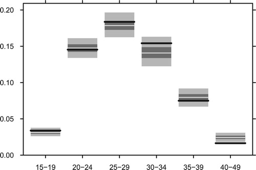
Figure 1 compares national-level age-specific fertility rates calculated from the census with rates calculated from the DHS. At all ages below 40, the DHS data imply substantially higher fertility rates than the census.

Figure 1. Direct estimates of age-specific fertility rates at the national level, based on the 2008 Census and 2010 Demographic and Health Survey.

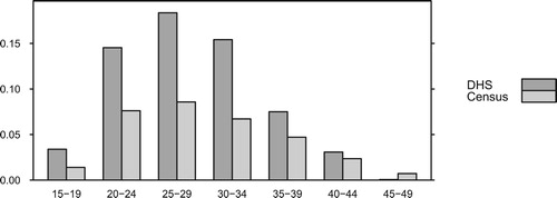
Figure 2 shows fertility rates calculated from census data. To save space, the figure only shows 8 of the 24 provinces. These provinces have similar but varying age profiles and have substantial variation in levels.

Figure 2. Direct estimates of age-specific fertility rates for eight selected provinces, based on the 2008 Census.

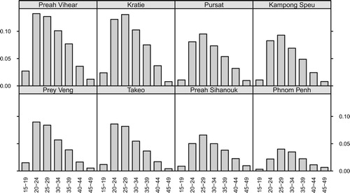
The provinces in Figure 2 are ordered by the proportion of the population below the poverty line (Asian Development Bank, 2014). The poorest province in Cambodia, Preah Vihear, has a poverty rate of 43.1%, and the wealthiest province in the country, Phnom Penh, has a poverty rate of 0.2%. Poorer provinces have higher fertility rates.

2.2. Overview of the model

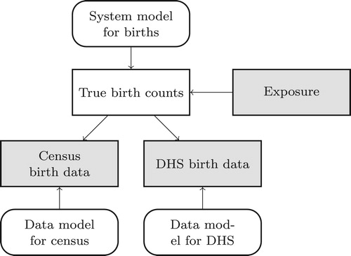
Our combined model contains a system model describing demographic processes, and data models describing measurement processes (Figure 3). The system model relates true birth counts to exposure, that is, to the number of women at the risk of giving birth. We treat exposure as known. The first data model describes the relationship between the true births counts and the census data. The second data model describes the relationship between the true births counts and the DHS data. We assume that errors in the census and errors in the DHS are independent, once we condition on the true birth counts.

Figure 3. An overview of the model for births in Cambodia. Straight-edged rectangles represent demographic arrays and rounded rectangles represent models. Grey shapes are observed; everything else must be inferred.

2.3. System model

We use $y_{ap}$ to denote the true, unobserved number of births to women aged a in province p. We assume that, conditional on exposure $w_{ap}$ and birth rates ${\gamma }_{ap}^{\mathrm{b}\mathrm{t}\mathrm{h}}$, birth counts $y_{ap}$ follow a Poisson distribution, (1) $y_{ap}\sim \mathrm{P}\mathrm{o}\mathrm{i}\mathrm{s}\mathrm{s}\mathrm{o}\mathrm{n}({\gamma }_{ap}^{\mathrm{b}\mathrm{t}\mathrm{h}}{w}_{ap}).$(1) We measure exposure using counts of women from the 2008 census.

Our system model is hierarchical, in that each unknown quantity in one level of the model is itself specified probabilistically in the next level of the model. Our specification for the birth rate ${\gamma }_{ap}^{\mathrm{b}\mathrm{t}\mathrm{h}}$ is linear on the log scale, with an intercept, an age effect, and a province effect, (2) $\log {\gamma }_{ap}^{\mathrm{b}\mathrm{t}\mathrm{h}}\sim \mathrm{N}({\beta }^{\mathrm{b}\mathrm{t}\mathrm{h},0}+{\beta }_a^{\mathrm{b}\mathrm{t}\mathrm{h},\mathrm{a}\mathrm{g}\mathrm{e}}+{\beta }_p^{\mathrm{b}\mathrm{t}\mathrm{h},\mathrm{p}\mathrm{r}\mathrm{o}\mathrm{v}},{\sigma }^2).$(2) Adding an age-province interaction to the model would be redundant in that Equation (2(2) $\log {\gamma }_{ap}^{\mathrm{b}\mathrm{t}\mathrm{h}}\sim \mathrm{N}({\beta }^{\mathrm{b}\mathrm{t}\mathrm{h},0}+{\beta }_a^{\mathrm{b}\mathrm{t}\mathrm{h},\mathrm{a}\mathrm{g}\mathrm{e}}+{\beta }_p^{\mathrm{b}\mathrm{t}\mathrm{h},\mathrm{p}\mathrm{r}\mathrm{o}\mathrm{v}},{\sigma }^2).$(2) ) is equivalent to (3) $\begin{array}{r}\log {\gamma }_{ap}^{\mathrm{b}\mathrm{t}\mathrm{h}}={\beta }^{\mathrm{b}\mathrm{t}\mathrm{h},0}+{\beta }_a^{\mathrm{b}\mathrm{t}\mathrm{h},\mathrm{a}\mathrm{g}\mathrm{e}}+{\beta }_p^{\mathrm{b}\mathrm{t}\mathrm{h},\mathrm{p}\mathrm{r}\mathrm{o}\mathrm{v}}+{\beta }_{ap}^{\mathrm{b}\mathrm{t}\mathrm{h},\mathrm{a}\mathrm{g}\mathrm{e}:\mathrm{p}\mathrm{r}\mathrm{o}\mathrm{v}}\end{array}$(3) with ${\beta }_{ap}^{\mathrm{b}\mathrm{t}\mathrm{h},\mathrm{a}\mathrm{g}\mathrm{e}:\mathrm{p}\mathrm{r}\mathrm{o}\mathrm{v}}\sim \mathrm{N}(0,{\sigma }^2)$. In other words, because $\log {\gamma }_{ap}$ is modelled as a draw from a normal distribution, our prior model already allows $\log {\gamma }_{ap}$ to depart from the value predicted by the age and province effects.

The intercept term ${\beta }^{\mathrm{b}\mathrm{t}\mathrm{h},0}$ is given the prior ${\beta }^{\mathrm{b}\mathrm{t}\mathrm{h},0}\sim \mathrm{N}(0,{10}^2)$. A value of 10 is large on a log scale, so this prior is highly diffuse.

The age effect ${\beta }_a^{\mathrm{b}\mathrm{t}\mathrm{h},\mathrm{a}\mathrm{g}\mathrm{e}}$ is defined using a ‘local trend’ time series model (Prado & West, 2010, pp. 119–120), (4) $\begin{array}{rl}{\beta }_a^{\mathrm{b}\mathrm{t}\mathrm{h},\mathrm{a}\mathrm{g}\mathrm{e}}& \sim \mathrm{N}({\alpha }_a,{\tau }_{\mathrm{a}\mathrm{g}\mathrm{e}}^2)\end{array}$(4) (5) $\begin{array}{rl}{\alpha }_a& \sim \mathrm{N}({\alpha }_{a-1}+{\delta }_a,{\omega }_{\alpha }^2)\end{array}$(5) (6) $\begin{array}{rl}{\delta }_a& \sim \mathrm{N}({\delta }_{a-1},{\omega }_{\delta }^2).\end{array}$(6) In (4(4) $\begin{array}{rl}{\beta }_a^{\mathrm{b}\mathrm{t}\mathrm{h},\mathrm{a}\mathrm{g}\mathrm{e}}& \sim \mathrm{N}({\alpha }_a,{\tau }_{\mathrm{a}\mathrm{g}\mathrm{e}}^2)\end{array}$(4) )–(6(6) $\begin{array}{rl}{\delta }_a& \sim \mathrm{N}({\delta }_{a-1},{\omega }_{\delta }^2).\end{array}$(6) ), ${\alpha }_a$'s are local level terms, and ${\delta }_a$'s are local trend terms. Both terms are not fixed for all age groups and are subject to random errors. The random error in ${\alpha }_a$ changes the mean of age effects for age group a and older age groups. The random error in ${\delta }_a$ changes the mean of differences in age effects between age groups a and a−1, and between older neighbouring age groups. Representing age effects with models developed originally for time series is common in statistical demography. Age effects, like time effects, tend to vary smoothly across neighbouring units, with a possibility of persistent upward or downward trends.

We allow the province effect to depend on provincial-level poverty rates, (7) ${\beta }_p^{\mathrm{b}\mathrm{t}\mathrm{h},\mathrm{p}\mathrm{r}\mathrm{o}\mathrm{v}}\sim \mathrm{N}(\alpha +\eta z_p,{\tau }_{\mathrm{p}\mathrm{r}\mathrm{o}\mathrm{v}}^2),$(7) where $z_p$ measures the poverty rate in province p, and parameter η captures the relationship between poverty and fertility. The variable $z_p$ is obtained by standardising the original poverty measure: we subtract off the mean, and divide through by 2 times the standard deviation.

All of the standard deviation terms in the system model receive ‘weakly informative’ half-t priors. A prior is weakly informative if it provides some guidance on the likely range of values for a parameter, but still understates our actual knowledge about that parameter (Gelman et al., 2014, pp. 55–57). A variable X has a half-t distribution with scale A and degrees of freedom ν if $X=A|Y|$ where $Y\sim t_{\nu }$. We set A = 1 and $\nu =7$ in all our priors for standard deviations. The coefficient η is given a t distribution, again with scale 1 and degrees of freedom 7.

2.4. Data models

The data model for the census counts predicts the number of births reported in the census, given the true number of births. We assume that births reported in the census, denoted by $x_{ap}^{\mathrm{c}\mathrm{e}\mathrm{n}}$, follow a Poisson distribution, (8) $x_{ap}^{\mathrm{c}\mathrm{e}\mathrm{n}}\sim \mathrm{P}\mathrm{o}\mathrm{i}\mathrm{s}\mathrm{s}\mathrm{o}\mathrm{n}({\gamma }_{ap}^{\mathrm{c}\mathrm{e}\mathrm{n}}{y}_{ap}).$(8) The parameter ${\gamma }_{ap}^{\mathrm{c}\mathrm{e}\mathrm{n}}$ measures the expected number of births appearing in the census for each birth that actually occurs. We refer to it as a coverage ratio. A value of 0.2, for instance, would imply that the census captured about 20% of births. As the ap subscripts indicate, we allow the coverage ratio to vary by age and province.

The ${\gamma }_{ap}^{\mathrm{c}\mathrm{e}\mathrm{n}}$ from Equation (8(8) $x_{ap}^{\mathrm{c}\mathrm{e}\mathrm{n}}\sim \mathrm{P}\mathrm{o}\mathrm{i}\mathrm{s}\mathrm{s}\mathrm{o}\mathrm{n}({\gamma }_{ap}^{\mathrm{c}\mathrm{e}\mathrm{n}}{y}_{ap}).$(8) ) has prior (9) $\begin{array}{r}\log {\gamma }_{ap}^{\mathrm{c}\mathrm{e}\mathrm{n}}\sim \mathrm{N}({\beta }^{\mathrm{c}\mathrm{e}\mathrm{n},0}+{\beta }_a^{\mathrm{c}\mathrm{e}\mathrm{n},\mathrm{a}\mathrm{g}\mathrm{e}}+{\beta }_p^{\mathrm{c}\mathrm{e}\mathrm{n},\mathrm{p}\mathrm{r}\mathrm{o}\mathrm{v}},{\sigma }_{\mathrm{c}\mathrm{e}\mathrm{n}}^2).\end{array}$(9) By including age effects ${\beta }_a^{\mathrm{c}\mathrm{e}\mathrm{n},\mathrm{a}\mathrm{g}\mathrm{e}}$ and province effects ${\beta }_p^{\mathrm{c}\mathrm{e}\mathrm{n},\mathrm{p}\mathrm{r}\mathrm{o}\mathrm{v}}$ in the model, we are allowing for the possibility that coverage ratios vary systematically by age and province.

The intercept term is given a diffuse prior, ${\beta }^{\mathrm{c}\mathrm{e}\mathrm{n},0}\sim \mathrm{N}(0,{10}^2)$. This implies that we do not have strong prior beliefs about the average coverage level of the census.

Our prior for the provincial effect is (10) ${\beta }_p^{\mathrm{c}\mathrm{e}\mathrm{n},\mathrm{p}\mathrm{r}\mathrm{o}\mathrm{v}}\sim \mathrm{N}(0,{\tau }_{\mathrm{c}\mathrm{e}\mathrm{n}}^2).$(10) We use an informative prior for ${\tau }_{\mathrm{c}\mathrm{e}\mathrm{n}}$: a half-t prior with 7 degrees of freedom and scale 0.05. This implies that we expect approximately 95% of provincial coverage ratios to be within 10 percent of the overall coverage ratio. It is often helpful to use informative priors when specifying data models. If the priors are too weak, then the model is unable to distinguish between variation in the underlying demographic rates and variation in coverage ratios.

We use a local level model for the age effect. A local level model is a special case of the local trend model with ${\delta }_a\equiv 0$. We expect neighbouring age groups to have similar coverage ratios, but do not expect a consistent trend upwards or downwards across age groups. As with the specification for provincial effects, we use informative priors on the standard deviation terms. We assume that the terms equivalent to τ and ${\omega }_{\alpha }$ in Equations (4(4) $\begin{array}{rl}{\beta }_a^{\mathrm{b}\mathrm{t}\mathrm{h},\mathrm{a}\mathrm{g}\mathrm{e}}& \sim \mathrm{N}({\alpha }_a,{\tau }_{\mathrm{a}\mathrm{g}\mathrm{e}}^2)\end{array}$(4) ) and (5(5) $\begin{array}{rl}{\alpha }_a& \sim \mathrm{N}({\alpha }_{a-1}+{\delta }_a,{\omega }_{\alpha }^2)\end{array}$(5) ) have half-t priors with 7 degrees of freedom and scale 0.05. These choices imply that we would not be surprised if neighbouring age groups had coverage ratios that differed by 20%, but would be surprised if they are different by, say, 100%.

Traditional demographic methods often make much stronger assumptions about errors in the data than the ones we make when setting up informative priors. In the section on the Cambodian census data, for instance, Moultrie et al. (2013) note that most traditional methods for estimating fertility rates assume that coverage ratios are identical across age groups, which, in our notation, is equivalent to assuming ${\gamma }_{a_0,p}^{\mathrm{c}\mathrm{e}\mathrm{n}}={\gamma }_{a_1,p}^{\mathrm{c}\mathrm{e}\mathrm{n}}$, all $a_0,a_1$.

Data for the 2010 Demographic and Health Survey were collected through a complicated process that involves stratification and community-level sampling. Given this complexity, a full Bayesian model of the relationship between the DHS data and the underlying fertility rates would require many more variables than just age and province. However, the DHS file contains sampling weights that, when analysed using classical methods for complex surveys, yield unbiased estimates and associated standard errors. We use functions from the R package survey(Lumley, 2004) to obtain a set of estimated age-specific birth counts $x_a^{\mathrm{d}\mathrm{h}\mathrm{s}}$ and associated standard errors $s_a$. Under the assumptions of the classical method, (11) $x_a^{\mathrm{d}\mathrm{h}\mathrm{s}}\sim \mathrm{N}(y_a,s_a^2).$(11) We use Equation (11(11) $x_a^{\mathrm{d}\mathrm{h}\mathrm{s}}\sim \mathrm{N}(y_a,s_a^2).$(11) ) as our data model for the DHS data.

Equation (11(11) $x_a^{\mathrm{d}\mathrm{h}\mathrm{s}}\sim \mathrm{N}(y_a,s_a^2).$(11) ) refers to age groups a, but not age-province combinations ap. In principle, we could disaggregate the DHS estimates by province as well. However, the classical method starts to produce unreliable estimates once cell sizes become small. Estimates of standard deviation terms from small cell sizes are particularly problematic.

The age group 45–49 requires special treatment. It turns out that the DHS sample for age 45–49 contains only three births. The classical method breaks down for a cell with such a small sample size. We therefore combine data for ages 40–44 and 45–49 in our data model, and use a pooled cell for age 40–49. Our estimation framework allows for the possibility that the age groups in a data model are less aggregated than the age groups in the system model.

The census refers to 2008 while the DHS refers to 2010. However, the DHS has a much more informative data model than the census, in that it makes much more precise claims about coverage rates. This implies that the overall level for fertility estimates from the model is essentially set by the DHS. Our results can therefore be interpreted as referring to 2010, rather than 2008. In principle, we could allow for changes in the age structure of provincial fertility rates and exposure between 2008 and 2010, but age structure change slowly over time, so the extra complexity would not be worthwhile.

2.5. Total fertility rate

The total fertility rate is a standard demographic summary measure for age-specific fertility rates. It is the average number of births a women would have over her lifetime if prevailing fertility rates were to continue indefinitely. It equals the sum of the age-specific rates, weighted by the number of years within each age group. For provincial data, with 5-year age groups, (12) ${\mathrm{T}\mathrm{F}\mathrm{R}}_p=5\sum _a{\gamma }_{ap}^{\mathrm{b}\mathrm{t}\mathrm{h}}.$(12) Once we have a posterior sample for the ${\gamma }_{ap}^{\mathrm{b}\mathrm{t}\mathrm{h}}$, obtaining a posterior sample for ${\mathrm{T}\mathrm{F}\mathrm{R}}_p$ is easy. For each draw of the ${\gamma }_{ap}^{\mathrm{b}\mathrm{t}\mathrm{h}}$, we simply calculate the associated value of ${\mathrm{T}\mathrm{F}\mathrm{R}}_p$. The resulting set of values forms the posterior sample for ${\mathrm{T}\mathrm{F}\mathrm{R}}_p$.

2.6. Computation

We fit models using our own R packages. The packages are both open source and are available at github.com/statisticsnz/R. The code for this paper is available at https://github.com/bayesiandemography/cambodiahttps://github.com/bayesiandemography/cambodia.

We use burnin of 200,000 iterations and production of 200,000 iterations, with 4 chains and thinning at a rate of 1/500. A relatively large number of iterations are required because of correlations between the latent birth counts and the demographic rates. The entire analysis takes less than 5 minutes on a 3.5 GHz Intel Core i5 iMac.

3. Results

Having fitted the model, we obtain samples from the posterior distribution of true birth counts $y_{ap}$, birth rates ${\gamma }_{ap}^{\mathrm{b}\mathrm{t}\mathrm{h}}$, census coverage ratios ${\gamma }_{ap}^{\mathrm{c}\mathrm{e}\mathrm{n}}$, and all the other parameters.

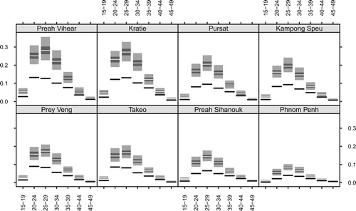
Figure 4 shows estimates of birth rates ${\gamma }_{ap}^{\mathrm{b}\mathrm{t}\mathrm{h}}$ for the eight selected provinces from Figure 2. The graphs show posterior medians, which serve as point estimates, and 95% and 50% credible intervals from the model. They also show the direct estimates from the census. For most of the age-province cells, the model estimates are higher than the direct estimates. Compared to the direct estimates, the model estimates indicate larger differences among age groups and also larger differences among provinces. The model estimates are higher in poorer provinces, such as Preah Vihear and Kratie, than richer provinces, such as Preah Sihanouk and Phnom Penh. Uncertainty in the model estimates, indicated by the length of credible intervals, is higher for the middle age groups and is higher for the poorer provinces.

Figure 4. Estimates of age-specific fertility rates for eight selected provinces. The light grey bands represent 95% credible intervals, the dark grey bands represent 50% credible intervals, and the pale lines represent posterior medians. The black lines represent direct estimates from the census.

For each age group a, Figure 5 shows the model estimates and the direct estimates from the DHS for the national-level fertility rate, $\sum _p{w}_{ap}{\gamma }_{ap}^{\mathrm{b}\mathrm{t}\mathrm{h}}/\sum _p{w}_{ap}$. We obtain a posterior sample for national-level rates in a way similar to that for obtaining a posterior sample for ${\mathrm{T}\mathrm{F}\mathrm{R}}_p$ described in Section 2.5. With one exception, the direct estimates from the DHS are all within the 95% credible intervals, which is consistent with our assumption that the DHS estimates are unbiased. The exception is the rate for ages 40–49, which, as discussed in Section 2.4, is more difficult to estimate from the DHS data. Uncertainty in the model estimates is higher for the middle age groups.

Figure 5. Estimates of age-specific fertility rates for the whole country. The black lines are direct estimates from the DHS.

We turn next to results from the data model for the census. Figure 6 shows estimates of coverage ratio ${\gamma }_{ap}^{\mathrm{c}\mathrm{e}\mathrm{n}}$. For most age-province cells, the estimates are well below one, confirming that the census undercounts the actual births. There is larger uncertainty in coverage ratio for the higher age groups, 40–44 and 45–49, reflecting the small sample sizes in these age groups, and the inconsistency between the DHS and census data. Across the provinces, there appears to be some difference in the age pattern for the coverage ratio. For instance, in Phnom Penh, the older the age group is, the higher the coverage ratio tends to be. However, in Preah Sihanouk, the coverage ratio is at a similar low level for the younger age groups and is higher for the older age groups.

Figure 6. Estimates of coverage ratios for census data in eight selected provinces.

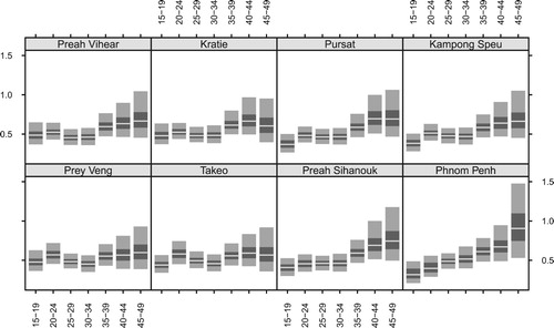
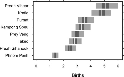
Figure 7 shows model estimates of ${\mathrm{T}\mathrm{F}\mathrm{R}}_p$ for the Cambodian provinces. The estimates are higher in poorer provinces than richer provinces. Preah Vihear and Kratie appear to have TFRs about 4 times higher than that in Phnom Penh. Uncertainty is higher for the poorer provinces.

Figure 7. Estimates of total fertility rates for eight selected provinces.

4. Discussion

The framework presented in this paper has a wide range of applications. It can, for instance, easily accommodate more than two datasets. In the Cambodian case, we could, for instance, extend the model to include multiple censuses and multiple surveys. Moreover, the datasets do not have to be censuses and surveys. Alternative sources of detailed demographic data include registration systems for births and deaths, household registration systems, and commercial data such as cell phone, social media, or electricity connection data.

A particular advantage of the framework described in the paper, in addition to its ability to cope with imperfect data sources, is the fact that it works at an aggregate level. There is no need to have individual-level data on people or events or to link together datasets at the individual level. This has both practical and ethical advantages.

The core of our framework is the set of unobserved true counts: in the Cambodian example, the set of unobserved true birth counts. Including these counts in the model allows us to separate the modelling of the underlying demographic processes from the modelling of the measurement errors in the data. This separation makes the framework more flexible and easier to understand when considered one submodel at time.

Bayesian MCMC methods allow us to construct an internally consistent posterior sample for all unknown quantities in the model, including the latent counts, the coverage ratios, and the demographic rates. This posterior sample can be used to construct detailed, coherent measures of uncertainty for all outputs from the model.

When accounting for measurement errors, we cannot avoid the need to make assumptions about likely biases or coverage ratios. However, the assumptions we make are typically weaker than those made in conventional demographic analyses, in that we specify ranges or distributions, rather than exact levels. Moreover, because the assumptions are set out in mathematical formula and computer code, the analysis is more transparent and reproducible.

Disclosure statement

No potential conflict of interest was reported by the authors.

Additional information

Notes on contributors

Junni L. Zhang

Junni L. Zhang is Associate Professor of Statistics at Peking University, China. Her research interests are Bayesian demography, causal inference, text and data mining. She has a PhD in Statistics from Harvard University.

John Bryant

John Bryant is a demographer and data scientist at Bayesian Demography Limited. He has previously worked at Statistics New Zealand, the New Zealand Treasury, and universities in New Zealand and Thailand. He has a PhD in Demography from the Australian National University.

References

- Asian Development Bank. (2014). Cambodia country poverty analysis 2014. Manila: Asian Development Bank.
- Bijak, J., & Bryant, J. (2016). Bayesian demography 250 years after Bayes. Population Studies, 70(1), 1–19. doi: 10.1080/00324728.2015.1122826
- Brick, J. M., Cervantes, I. F., Lee, S., & Norman, G. (2011). Nonsampling errors in dual frame telephone surveys. Survey Methodology, 37, 1–12.
- Bryant, J., & Zhang, J. L. (2018). Bayesian demographic estimation and forecasting. Boca Raton: CRC Press.
- Christen, P. (2012). Data matching: Concepts and techniques for record linkage, entity resolution, and duplicate detection. New York, NY: Springer Science and Business Media.
- Dwyer-Lindgren, L., Squires, E. R., Teeple, S., Ikilezi, G., Roberts, D. A., Colombara, D. V., …Lim, S. S. (2018). Small area estimation of under-5 mortality in Bangladesh, Cameroon, Chad, Mozambique, Uganda, and Zambia using spatially misaligned data. Population Health Metrics, 16(13), 1–15.
- Fay, R. E. I., & Herriot, R. A. (1979). Estimates of income for small places: An application of James–Stein procedures to census data. Journal of the American Statistical Association, 74, 269–277. doi: 10.1080/01621459.1979.10482505
- Gelman, A., Carlin, J., Stern, H., Dunson, D. B., Vehtari, A., & Rubin, D. (2014). Bayesian data analysis (3rd ed.). New York, NY: Chapman and Hall.
- Gelman, A., King, G., & Liu, C. (1998). Not asked and not answered: Multiple imputation for multiple surveys. Journal of the American Statistical Association, 93, 846–857. doi: 10.1080/01621459.1998.10473737
- Harron, K., Goldstein, H., & Dibben, C. (2016). Methodological developments in data linkage. Hoboken, NJ: Wiley.
- He, Y., Landrum, M. B., & Zaslavsky, A. M. (2014). Combining information from two data sources with misreporting and incompleteness to assess hospice-use among cancer patients: A multiple imputation approach. Statistics in Medicine, 33, 3710–3724. doi: 10.1002/sim.6173
- Herzog, T. N., Scheuren, F. J., & Winkler, W. E. (2017). Data quality and record linkage techniques. New York, NY: Springer Science and Business Media.
- Kim, J. K., Park, S., & Kim, S. Y. (2015). Small area estimation combining information from several sources. Survey Methodology, 41(1), 21–36.
- Kim, J. K., & Rao, J. N. K. (2012). Combining data from two independent surveys: A model-assisted approach. Biometrika, 99, 85–100. doi: 10.1093/biomet/asr063
- Knutson, K., Zhang, W., & Tabnak, F. (2008). Applying the small-area estimation method to estimate a population eligible for breast cancer detection. Preventing Chronic Disease, 5(1), A10.
- Lesser, V. M., Newton, L., & Yang, D (2008). Evaluating frames and modes of contact in a study of individuals with disabilities. Paper presented at the Joint Statistical Meetings, Denver, CO.
- Lohr, S. L., & Raghunathan, T. E. (2017). Combining survey data with other data sources. Statistical Science, 32(2), 293–312. doi: 10.1214/16-STS584
- Lohr, S. L., & Rao, J. N. K. (2006). Estimation in multiple-frame surveys. Journal of the American Statistical Association, 101, 1019–1030. doi: 10.1198/016214506000000195
- Lumley, T. (2004). Analysis of complex survey samples. Journal of Statistical Software, 9(1), 1–19.
- Lynch, S. M., & Brown, J. S. (2010). Obtaining multistate life table distributions for highly refined subpopulations from cross-sectional data: A Bayesian extension of Sullivan's method. Demography, 47(4), 1053–1077. doi: 10.1007/BF03213739
- Manzi, G., Spiegelhalter, D. J., Turner, R. M., Flowers, J., & Thompson, S. G. (2011). Modelling bias in combining small area prevalence estimates from multiple surveys. Journal of the Royal Statistical Society: Series A, 174(1), 31–50. doi: 10.1111/j.1467-985X.2010.00648.x
- Metcalf, P., & Scott, A. (2009). Using multiple frames in health surveys. Statistics in Medicine, 28, 1512–1523. doi: 10.1002/sim.3566
- Moultrie, T. A., Dorrington, R., Hill, A., Hill, K., Timæus, I., & Zaba, B. (2013). Tools for demographic estimation. Paris: International Union for the Scientific Study of Population.
- National Institute of Statistics, Directorate General for Health, & ICF Macro. (2011a). Cambodia demographic and health survey 2010. Author.
- National Institute of Statistics, Directorate General for Health, & ICF Macro (2011b). Cambodia demographic and health survey 2010 [Dataset] (khir61fl.dta). Author.
- Pfeffermann, D. (2013). New important developments in small area estimation. Statistical Science, 28(1), 40–68. doi: 10.1214/12-STS395
- Prado, R., & West, M. (2010). Time series: Modeling, computation, and inference. Boca Raton, FL: CRC Press.
- Preston, S., Heuveline, P., & Guillot, M. (2001). Demography: Modelling and measuring population processes. Oxford: Blackwell.
- Raghunathan, T. E. (2006). Combining information from multiple surveys for assessing health disparities. Allgemeines Statistisches Archiv, 90, 515–526. doi: 10.1007/s10182-006-0003-0
- Raghunathan, T., Xie, D., Schenker, N., Parsons, V., Davis, W., Dodd, K., & Feuer, E. (2007). Combining information from two surveys to estimate county-level prevalence rates of cancer risk factors and screening. Journal of the American Statistical Association, 102, 474–486. doi: 10.1198/016214506000001293
- Ranalli, M. G., Arcos, A., Rueda, M. D. M., & Teodoro, A. (2016). Calibration estimation in dual-frame surveys. Statistical Methods and Applications, 25, 321–349. doi: 10.1007/s10260-015-0336-5
- Rao, J. N. K., & Molina, I. (2015). Small area estimation (2nd ed.). Hoboken: John Wiley & Sons.
- Schenker, N., Raghunathan, T. E., & Bondarenko, I. (2010). Improving on analyses of self-reported data in a large-scale health survey by using information from an examination-based survey. Statistics in Medicine, 29, 533–545.
- Schmertmann, C. P., Cavenaghi, S. M., Assunção, R. M., & Potter, J. E. (2013). Bayes plus Brass: Estimating total fertility for many small areas from sparse census data. Population Studies, 67(3), 255–273. doi: 10.1080/00324728.2013.795602
- Steorts, R. C., Hall, R., & Fienberg, S. E. (2016). A Bayesian approach to graphical record linkage and de-duplication. Journal of the American Statistical Association, 111, 1660–1672. doi: 10.1080/01621459.2015.1105807
- Zhang, J. L., Bryant, J., & Nissen, K. (2019). Bayesian small area demography. Survey Methodology, 45(1), 13–29.