Small area estimation with subgroup analysis

ABSTRACT

In this article, a new unit level model based on a pairwise penalised regression approach is proposed for problems in small area estimation (SAE). Instead of assuming common regression coefficients for all small domains in the traditional model, the new estimator is based on a subgroup regression model which allows different regression coefficients in different groups. The alternating direction method of multipliers (ADMM) algorithm is used to find subgroups with different regression coefficients. We also consider pairwise spatial weights for spatial areal data. In the simulation study, we compare the performances of the new estimator with the traditional small area estimator. We also apply the new estimator to urban area estimation using data from the National Resources Inventory survey in Iowa.

KEYWORDS:

• Linear mixed models
• penalty regressions
• small area estimation
• spatial areal data
• subgroup analysis

1. Introduction

Small area estimation (SAE) is an important problem in survey sampling when the sample sizes are not large enough to provide reliable estimates in small domains or areas. See Rao and Molina (2015) and Pfeffermann (2013) for overviews and recent developments in SAE. One of the model-based approaches for SAE is the unit level model, which was first proposed by Battese, Harter, and Fuller (1988). Unit level models are specified for the individual elements of the population and require the availability of unit level auxiliary information.

Traditional unit level models typically assume a linear relationship between the variable of interest and the auxiliary information, and all the areas share the same regression coefficients to borrow information. Random effects are also considered for each small area. However, different relationships can exist in different areas. That is, subgroups could exist for different areas such that areas in one group have the same regression coefficient and areas in different groups have different regression coefficients.

In the linear regression setting, Ma and Huang (2017), Ma, Huang, and Zhang (2016) developed a method to obtain homogeneous groups based on regression coefficients through the alternating direction method of multiplier algorithm (ADMM, Boyd, Parikh, Chu, Peleato, & Eckstein, 2011). In the algorithm, they used pairwise concave penalties based on the smoothly clipped absolute deviation (SCAD) penalty (Fan & Li, 2001) and the minimax concave penalty (MCP) (Zhang, 2010). Wang, Zhu, and Zhang (2019) extended the problem to a regression setting with repeated measures. They also considered spatial weights in the pairwise penalties and showed that spatial weights perform better than equal weights. However, the model cannot be applied to the SAE problems directly, since random effects are not considered.

In this article, we propose a new SAE estimator that allows different regression coefficients in different subgroups under a linear mixed model framework at the unit level. The ADMM algorithm is applied and the variance parameters are also estimated in the algorithm. As in Wang et al. (2019), we use spatial pairwise weights in the pairwise penalties based on the SCAD penalty. In this algorithm, the number of groups and the group structure are also determined.

The article is organised as follows. In Section 2, we introduce the unit level model with areal regression coefficients and the algorithm to find subgroups. In Section 3, we conduct several simulation studies to compare the performance of the proposed estimator with the traditional estimators. In Section 4, we apply the proposed method to a real data set. Finally, Section 5 contains some conclusion and discussion.

2. The model and the algorithm

In this section, the unit level model with area level regression coefficients and the corresponding algorithm to estimate parameters are introduced.

2.1. The unit level model

Suppose there are M areas with known population size $N_i$ and $n_i$ is the sample size in area i for $i=1,\dots ,M$. Let $y_{ih}$ be the observation of unit h in area i for $h=1,\dots ,n_i$, $i=1,\dots ,M$. Let ${\mathit{x}}_{ih}$ be the p dimension auxiliary information vector with area population mean ${\overline{\mathit{X}}}_i=1/N_i\sum _{h=1}^{N_i}{\mathit{x}}_{ih}$ known. In the traditional unit level model, that is Battese–Harter–Fuller (BHF) model (Battese et al., 1988), different areas share the same regression coefficient as in (1(1) $y_{ih}={\mathit{x}}_{ih}^{\mathrm{T}}\mathit{\beta }+v_i+{ϵ}_{ih},$(1) ), (1) $y_{ih}={\mathit{x}}_{ih}^{\mathrm{T}}\mathit{\beta }+v_i+{ϵ}_{ih},$(1) where $\mathit{\beta }$ is the unknown regression coefficient vector, $v_i$'s are i.i.d areal random effects with mean zero and variance ${\sigma }_v^2$, and ${ϵ}_{ih}$'s are i.i.d random errors with mean zero and variance ${\sigma }_{ϵ}^2$. Let $A_i$ be the set of observed units and $C_i$ be the set of unobserved units in area i. The predictor for the finite population mean ${\overline{Y}}_i=1/N_i\sum _{h=1}^{N_i}{y}_{ih}$ in area i under model (1(1) $y_{ih}={\mathit{x}}_{ih}^{\mathrm{T}}\mathit{\beta }+v_i+{ϵ}_{ih},$(1) ) for SAE given in Battese et al. (1988) and the sae package (Molina & Marhuenda, 2015) is (2) ${\hat{\overline{Y}}}_i^{\mathrm{B}\mathrm{H}\mathrm{F}}=\frac{1}{N_i}\left(\sum _{h\in A_i}{y}_{ih}+\sum _{h\in C_i}\left({\mathit{x}}_{ih}^{\mathrm{T}}\hat{\mathit{\beta }}+{\hat{v}}_i\right)\right),$(2) where $\hat{\mathit{\beta }}$ is the estimate of $\mathit{\beta }$ and ${\hat{v}}_i$ is the empirical best linear unbiased prediction of $v_i$. In the simulation study, we use the R package sae (Molina & Marhuenda, 2015) to obtain the predictions.

Instead of assuming all the areas have the same regression coefficients $\mathit{\beta }$, we assume that there are K mutually exclusive subgroups $\mathcal{G}=\{{\mathcal{G}}_1,\dots ,{\mathcal{G}}_K\}$, which is a partition of areas $\{1,2,\dots ,M\}$. First we assume that each area has its own regression coefficient, (3) $y_{ih}={\mathit{x}}_{ih}^{\mathrm{T}}{\mathit{\beta }}_i+v_i+{ϵ}_{ih},$(3) where ${\mathit{\beta }}_i$ is the unknown regression coefficient vector for area i. Let ${\mathit{y}}_i=(y_{i1},\dots ,y_{i{n}_i}{)}^{\mathrm{T}}$, ${\mathit{x}}_i=({\mathit{x}}_{i1},\dots ,{\mathit{x}}_{i{n}_i}{)}^{\mathrm{T}}$ and $\mathit{\beta }=({\mathit{\beta }}_1^{\mathrm{T}},\dots ,{\mathit{\beta }}_M^{\mathrm{T}}{)}^{\mathrm{T}}$. The weighted log likelihood function is (4) $\begin{array}{rl}l\left(\mathit{\beta },{\sigma }_v^2,{\sigma }_{ϵ}^2\right)& =-\frac{1}{2}\sum _{i=1}^M\frac{1}{n_i}\log \left|{\mathrm{\Sigma }}_i\right|\\ & -\frac{1}{2}\sum _{i=1}^M\frac{1}{n_i}{\left({\mathit{y}}_i-{\mathit{x}}_i^{\mathrm{T}}{\mathit{\beta }}_i\right)}^{\mathrm{T}}\\ & \times {\mathrm{\Sigma }}_i^{-1}\left({\mathit{y}}_i-{\mathit{x}}_i^{\mathrm{T}}{\mathit{\beta }}_i\right),\end{array}$(4) where ${\mathrm{\Sigma }}_i$ is the covariance matrix based on the random effect structure which has the following form: ${\mathrm{\Sigma }}_i={\mathbf{1}}_{n_i}{\mathbf{1}}_{n_i}^{\mathrm{T}}{\sigma }_v^2+{\mathit{I}}_{n_i}{\sigma }_{ϵ}^2$ and $\begin{array}{rl}{\mathrm{\Sigma }}_i^{-1}& ={\left({\mathbf{1}}_{n_i}{\mathbf{1}}_{n_i}^{\mathrm{T}}{\sigma }_v^2+{\mathit{I}}_{n_i}{\sigma }_{ϵ}^2\right)}^{-1}\\ & =\frac{1}{{\sigma }_{ϵ}^2}\left({\mathit{I}}_{n_i}-{\mathbf{1}}_{n_i}{\mathbf{1}}_{n_i}^{\mathrm{T}}\frac{{\sigma }_v^2}{{\sigma }_{ϵ}^2+n_i{\sigma }_v^2}\right),\end{array}$ where ${\mathbf{1}}_{n_i}$ is an $n_i\times 1$ vector with elements 1 and ${\mathit{I}}_{n_i}$ is an $n_i\times n_i$ identity matrix.

If area i and area j are in the same group, then ${\mathit{\beta }}_i={\mathit{\beta }}_j$. In order to find the estimated partition $\hat{\mathcal{G}}=\{{\hat{\mathcal{G}}}_1,\dots ,{\hat{\mathcal{G}}}_{\hat{K}}\}$ with the estimated number of groups $\hat{K}$, the following objective function is considered (5) $\begin{array}{rl}& Q\left(\mathit{\beta },{\sigma }_v^2,{\sigma }_{ϵ}^2;\lambda ,\psi \right)\\ & =\frac{1}{2}\sum _{i=1}^M\frac{1}{n_i}\log \left|{\mathrm{\Sigma }}_i\right|+\frac{1}{2}\sum _{i=1}^M\frac{1}{n_i}{\left({\mathit{y}}_i-{\mathit{x}}_i^{\mathrm{T}}{\mathit{\beta }}_i\right)}^{\mathrm{T}}\\ & \times {\mathrm{\Sigma }}_i^{-1}\left({\mathit{y}}_i-{\mathit{x}}_i^{\mathrm{T}}{\mathit{\beta }}_i\right)\\ & +\sum _{1\le i<j\le M}{p}_{\gamma }\left(∥{\mathit{\beta }}_i-{\mathit{\beta }}_j∥,c_{ij}\lambda \right),\end{array}$(5) where $\parallel \cdot \parallel$ denotes the Euclidean norm, $p_{\gamma }(\cdot ,\lambda )$ is a penalty function with a fixed value γ and a tuning parameter $\lambda \ge 0$. In the penalty function, pairwise weights are considered associated with area i and area j. In this paper, we use the SCAD penalty. In the context of spatial SAE, we define $c_{ij}$ as (6) $c_{ij}=\exp \left(\psi (1-a_{ij})\right),$(6) where ψ is a tuning parameter and $a_{ij}$ is the neighbour order between area i and area j. As shown in Wang et al. (2019), pairwise spatial weights can help in spatial areal data.

2.2. The ADMM algorithm

For given λ and ψ, the solution of (5(5) $\begin{array}{rl}& Q\left(\mathit{\beta },{\sigma }_v^2,{\sigma }_{ϵ}^2;\lambda ,\psi \right)\\ & =\frac{1}{2}\sum _{i=1}^M\frac{1}{n_i}\log \left|{\mathrm{\Sigma }}_i\right|+\frac{1}{2}\sum _{i=1}^M\frac{1}{n_i}{\left({\mathit{y}}_i-{\mathit{x}}_i^{\mathrm{T}}{\mathit{\beta }}_i\right)}^{\mathrm{T}}\\ & \times {\mathrm{\Sigma }}_i^{-1}\left({\mathit{y}}_i-{\mathit{x}}_i^{\mathrm{T}}{\mathit{\beta }}_i\right)\\ & +\sum _{1\le i<j\le M}{p}_{\gamma }\left(∥{\mathit{\beta }}_i-{\mathit{\beta }}_j∥,c_{ij}\lambda \right),\end{array}$(5) ) is (7) $\begin{array}{rl}\left(\hat{\mathit{\beta }},\widehat{{\sigma }_v^2},\widehat{{\sigma }_{ϵ}^2}\right)& =\underset{\mathit{\beta }\in {\mathbb{R}}^{Mp},{\sigma }_v^2\in {\mathbb{R}}_{+},{\sigma }_{ϵ}^2\in {\mathbb{R}}_{+}}{\mathrm{a}\mathrm{r}\mathrm{g}\mathrm{m}\mathrm{i}\mathrm{n}}\\ & Q\left(\mathit{\beta },{\sigma }_v^2,{\sigma }_{ϵ}^2;\lambda ,\psi \right).\end{array}$(7) The ADMM algorithm is applied to solve (7(7) $\begin{array}{rl}\left(\hat{\mathit{\beta }},\widehat{{\sigma }_v^2},\widehat{{\sigma }_{ϵ}^2}\right)& =\underset{\mathit{\beta }\in {\mathbb{R}}^{Mp},{\sigma }_v^2\in {\mathbb{R}}_{+},{\sigma }_{ϵ}^2\in {\mathbb{R}}_{+}}{\mathrm{a}\mathrm{r}\mathrm{g}\mathrm{m}\mathrm{i}\mathrm{n}}\\ & Q\left(\mathit{\beta },{\sigma }_v^2,{\sigma }_{ϵ}^2;\lambda ,\psi \right).\end{array}$(7) ). Let ${\mathit{\delta }}_{ij}={\mathit{\beta }}_i-{\mathit{\beta }}_j$, the objective function becomes $\begin{array}{rl}& L_0\left(\mathit{\beta },{\sigma }_v^2,{\sigma }_{ϵ}^2,\mathit{\delta }\right)\\ & =\frac{1}{2}\sum _{i=1}^M\frac{1}{n_i}\log \left|{\mathrm{\Sigma }}_i\right|\\ & +\frac{1}{2}\sum _{i=1}^M\frac{1}{n_i}{\left({\mathit{y}}_i-{\mathit{x}}_i^{\mathrm{T}}{\mathit{\beta }}_i\right)}^{\mathrm{T}}{\mathrm{\Sigma }}_i^{-1}\left({\mathit{y}}_i-{\mathit{x}}_i^{\mathrm{T}}{\mathit{\beta }}_i\right)\\ & +\sum _{1\le i<j\le M}{p}_{\gamma }\left(∥{\mathit{\delta }}_{ij}∥,c_{ij}\lambda \right)\\ & \mathrm{s}\mathrm{u}\mathrm{b}\mathrm{j}\mathrm{e}\mathrm{c}\mathrm{t}\mathrm{t}\mathrm{o}{\mathit{\beta }}_i-{\mathit{\beta }}_j-{\mathit{\delta }}_{ij}=\mathbf{0},\end{array}$ where $\mathit{\delta }=({\mathit{\delta }}_{ij}^{\mathrm{T}},i<j{)}^{\mathrm{T}}$. The augmented Lagrangian is $\begin{array}{rl}L\left(\mathit{\beta },{\sigma }_v^2,{\sigma }_{ϵ}^2,\mathit{\delta },\mathit{v}\right)& =L_0\left(\mathit{\beta },{\sigma }_v^2,{\sigma }_{ϵ}^2,\mathit{\delta }\right)\\ & +\sum _{i<j}⟨{\mathit{v}}_{ij},{\mathit{\beta }}_i-{\mathit{\beta }}_j-{\mathit{\delta }}_{ij}⟩\\ & +\frac{\vartheta }{2}\sum _{i<j}\parallel {\mathit{\beta }}_i-{\mathit{\beta }}_j-{\mathit{\delta }}_{ij}{\parallel }^2,\end{array}$ where $\mathit{v}=({\mathit{v}}_{ij}^{\mathrm{T}},i<j{)}^{\mathrm{T}}$ are Lagrange multipliers and ϑ is the penalty parameter. Let $\mathit{\tau }=({\sigma }_v^2,{\sigma }_{ϵ}^2)$. Given ${\mathit{\tau }}^m$, ${\mathit{\delta }}^m$ and ${\mathit{v}}^m$, $\mathit{\beta },\mathit{\tau },\mathit{\delta }$ and $\mathit{v}$ are updated as follows: $\begin{array}{rl}{\mathit{\beta }}^{m+1}& =\arg minL\left(\mathit{\beta },{\mathit{\tau }}^m,{\mathit{\delta }}^m,{\mathit{v}}^m\right),\\ {\mathit{\tau }}^{m+1}& ={\mathit{\tau }}^m+{\left[\mathcal{I}\left({\mathit{\tau }}^m\right)\right]}^{-1}s\left({\mathit{\beta }}^{m+1},{\mathit{\tau }}^m\right),\\ {\mathit{\delta }}^{m+1}& =\arg minL\left({\mathit{\beta }}^{m+1},{\mathit{\tau }}^{m+1},\mathit{\delta },{\mathit{v}}^m\right),\\ {\mathit{v}}_{ij}^{m+1}& ={\mathit{v}}_{ij}^m+\vartheta \left({\mathit{\beta }}_i^{m+1}-{\mathit{\beta }}_j^{m+1}-{\mathit{\delta }}_{ij}^{m+1}\right).\end{array}$ Let $\mathit{y}=({\mathit{y}}_1^{\mathrm{T}},\dots ,{\mathit{y}}_M^{\mathrm{T}}{)}^{\mathrm{T}}$, $\mathit{X}=\mathrm{d}\mathrm{i}\mathrm{a}\mathrm{g}({\mathit{x}}_1,{\mathit{x}}_2,\dots ,{\mathit{x}}_M)$ and $\mathbf{\Omega }=\mathrm{d}\mathrm{i}\mathrm{a}\mathrm{g}(1/n_1{\mathrm{\Sigma }}_1^{-1},\dots ,1/n_M{\mathrm{\Sigma }}_M^{-1})$. The update of $\mathit{\beta }$ is $\begin{array}{rl}{\mathit{\beta }}^{m+1}& ={\left({\mathit{X}}^{\mathrm{T}}{\mathbf{\Omega }}^m\mathit{X}+\vartheta {\mathit{A}}^{\mathrm{T}}\mathit{A}\right)}^{-1}\\ & \times \left({\mathit{X}}^{\mathrm{T}}{\mathbf{\Omega }}^m\mathit{y}+\vartheta \mathrm{v}\mathrm{e}\mathrm{c}\left(\left({\mathbf{\Delta }}^m-{\vartheta }^{-1}{\mathit{{\rm Y}}}^m\right)\mathit{D}\right)\right),\end{array}$ where $\mathit{A}=\mathit{D}\otimes {\mathit{I}}_p$, ⊗ is the Kronecker product, $\mathit{D}=\left\{\right({\mathit{e}}_i-{\mathit{e}}_j){\}}^{\mathrm{T}}$ with ${\mathit{e}}_i$ an $M\times 1$ vector with ith element 1 and other elements 0, ${\mathbf{\Delta }}^m=({\mathit{\delta }}_{ij}^m,i<j{)}_{p\times M(M-1)/2}$ and ${\mathit{{\rm Y}}}^m=({\mathit{v}}_{ij}^m,i<j{)}_{p\times M(M-1)/2}$. When updating $\mathit{\tau }$, $\mathcal{I}\mathcal{\left(}\mathit{\tau }\mathcal{\right)}$ is the expected second-order derivative of $-l$ in (4(4) $\begin{array}{rl}l\left(\mathit{\beta },{\sigma }_v^2,{\sigma }_{ϵ}^2\right)& =-\frac{1}{2}\sum _{i=1}^M\frac{1}{n_i}\log \left|{\mathrm{\Sigma }}_i\right|\\ & -\frac{1}{2}\sum _{i=1}^M\frac{1}{n_i}{\left({\mathit{y}}_i-{\mathit{x}}_i^{\mathrm{T}}{\mathit{\beta }}_i\right)}^{\mathrm{T}}\\ & \times {\mathrm{\Sigma }}_i^{-1}\left({\mathit{y}}_i-{\mathit{x}}_i^{\mathrm{T}}{\mathit{\beta }}_i\right),\end{array}$(4) ) and $s\left({\mathit{\beta }}^{m+1},{\mathit{\tau }}^m\right)={\left(\frac{\mathrm{\partial }l}{\mathrm{\partial }{\sigma }_v^2},\frac{\mathrm{\partial }l}{\mathrm{\partial }{\sigma }_{ϵ}^2}\right)}^{\mathrm{T}}{|}_{\mathit{\beta }={\mathit{\beta }}^{m+1},\mathit{\tau }={\mathit{\tau }}^m}.$ The details of $s(\cdot ,\cdot )$ and $\mathcal{I}$ are in the appendix. In this step, $\mathit{\tau }$ can be updated several times within one iteration.

Updating ${\mathit{\delta }}_{ij}$ is based on the result of SCAD penalty. Let ${\mathit{\varsigma }}_{ij}^m=({\mathit{\beta }}_i^{m+1}-{\mathit{\beta }}_j^{m+1})+{\vartheta }^{-1}{\mathit{v}}_{ij}^m$, then the solution is

${\mathit{\delta }}_{ij}^{m+1}=\left\{\begin{array}{ll}S\left({\mathit{\varsigma }}_{ij}^m,\lambda c_{ij}/\vartheta \right)& \mathrm{i}\mathrm{f}∥{\mathit{\varsigma }}_{ij}^m∥\le \lambda c_{ij}+\lambda c_{ij}/\vartheta ,\\ \frac{S\left({\mathit{\varsigma }}_{ij}^m,\gamma \lambda c_{ij}/\left(\left(\gamma -1\right)\vartheta \right)\right)}{1-1/\left(\left(\gamma -1\right)\vartheta \right)}& \mathrm{i}\mathrm{f}\lambda c_{ij}+\lambda c_{ij}/\vartheta <∥{\mathit{\varsigma }}_{ij}^m∥\le \gamma \lambda c_{ij},\\ {\mathit{\varsigma }}_{ij}^m& \mathrm{i}\mathrm{f}∥{\mathit{\varsigma }}_{ij}^m∥>\gamma \lambda c_{ij},\end{array}\right.$where $\gamma >c_{ij}+c_{ij}/\vartheta$ and $S(\mathit{w},t)=(1-t/\parallel \mathit{w}\parallel {)}_{+}\mathit{w}$ and $(t{)}_{+}=t$ if t>0, 0 otherwise.

Remark 2.1

The convergence criteria is based on that given in Boyd et al. (2011). The primal residual and dual residual are defined as ${\mathit{r}}^{m+1}=\mathit{A}{\mathit{\beta }}^{m+1}-{\mathit{\delta }}^{m+1}$ and ${\mathit{s}}^{m+1}=\vartheta {\mathit{A}}^{\mathrm{T}}({\mathit{\delta }}^{m+1}-{\mathit{\delta }}^m)$. The stopping criterion is ${∥{\mathit{r}}^m∥}_2\le {ϵ}^{\mathrm{p}\mathrm{r}\mathrm{i}},{∥{\mathit{s}}^m∥}_2\le {ϵ}^{\mathrm{d}\mathrm{u}\mathrm{a}\mathrm{l}},$ where $\begin{array}{rl}{ϵ}^{\mathrm{p}\mathrm{r}\mathrm{i}}& =\sqrt{\frac{M\left(M-1\right)}{2}p}{ϵ}^{\mathrm{a}\mathrm{b}\mathrm{s}}\\ & +{ϵ}^{\mathrm{r}\mathrm{e}\mathrm{l}}max\left\{∥\mathit{A}{\mathit{\beta }}^m∥,∥{\mathit{\delta }}^m∥\right\},\\ {ϵ}^{\mathrm{d}\mathrm{u}\mathrm{a}\mathrm{l}}& =\sqrt{Mp}{ϵ}^{\mathrm{a}\mathrm{b}\mathrm{s}}+{ϵ}^{\mathrm{r}\mathrm{e}\mathrm{l}}∥{\mathit{A}}^{\mathrm{T}}{\mathit{v}}^m∥,\end{array}$where ${ϵ}^{\mathrm{a}\mathrm{b}\mathrm{s}}$ is an absolute tolerance and ${ϵ}^{\mathrm{r}\mathrm{e}\mathrm{l}}$ is a relative tolerance. In the simulation study and the application, we use ${ϵ}^{\mathrm{a}\mathrm{b}\mathrm{s}}={10}^{-4}$ and ${ϵ}^{\mathrm{r}\mathrm{e}\mathrm{l}}={10}^{-2}$.

2.3. The proposed small area estimator

As in Zhu, Zou, Liang, and Zhu (2016), two small area estimators can be defined. Let ${\overline{y}}_i=1/n_i\sum _{h=1}^{n_i}{y}_{ih}$ and ${\overline{\mathit{x}}}_i=1/n_i\sum _{h=1}^{n_i}{\mathit{x}}_{ih}$ be the sample mean of the variable of interest and auxiliary information, respectively. The first one is based on the predictions of random effects, which is defined as (8) ${\hat{\overline{Y}}}_i^{\left(1\right)}={\overline{\mathit{X}}}_i^{\mathrm{T}}{\hat{\mathit{\beta }}}_i+{\hat{v}}_i,$(8) where ${\hat{\mathit{\beta }}}_i$ is the estimate of ${\mathit{\beta }}_i$ from the proposed algorithm, ${\hat{v}}_i={\hat{\gamma }}_i\left({\overline{y}}_i-{\overline{\mathit{x}}}_i^{\mathrm{T}}{\hat{\mathit{\beta }}}_i\right),$ and ${\hat{\gamma }}_i={\hat{\sigma }}_v^2/({\hat{\sigma }}_v^2+{\hat{\sigma }}_{ϵ}^2/n_i).$

In the second estimator, the unobserved values in each area are predicted based on the model, which is given by (9) $\begin{array}{rl}{\hat{\overline{Y}}}_i^{\left(2\right)}& =\frac{1}{N_i}\left(\sum _{h\in A_i}{y}_{ih}+\sum _{h\in C_i}{\hat{y}}_{ih}\right)\\ & =f_i{\overline{y}}_i+{\left({\overline{\mathit{X}}}_i-f_i\overline{{\mathit{x}}_i}\right)}^{\mathrm{T}}{\hat{\mathit{\beta }}}_i+\left(1-f_i\right){\hat{v}}_i,\end{array}$(9) where ${\hat{y}}_{ih}={\mathit{x}}_{ih}^{\mathrm{T}}{\hat{\mathit{\beta }}}_i+{\hat{v}}_i$ and $f_i=n_i/N_i$. If $f_i$ is small, then the predictor in (9(9) $\begin{array}{rl}{\hat{\overline{Y}}}_i^{\left(2\right)}& =\frac{1}{N_i}\left(\sum _{h\in A_i}{y}_{ih}+\sum _{h\in C_i}{\hat{y}}_{ih}\right)\\ & =f_i{\overline{y}}_i+{\left({\overline{\mathit{X}}}_i-f_i\overline{{\mathit{x}}_i}\right)}^{\mathrm{T}}{\hat{\mathit{\beta }}}_i+\left(1-f_i\right){\hat{v}}_i,\end{array}$(9) ) is nearly identical to the predictor in (8(8) ${\hat{\overline{Y}}}_i^{\left(1\right)}={\overline{\mathit{X}}}_i^{\mathrm{T}}{\hat{\mathit{\beta }}}_i+{\hat{v}}_i,$(8) ).

3. Simulation study

The simulation setup is designed based on the features of the National Resources Inventory (NRI) survey, which monitors status and trend of natural resources characteristics. One of the characteristic is the area of land uses, such as cropland, pastureland and urban (Nusser & Goebel, 1997). Each state is divided into ‘segments’ with size of 160 acres. From 1982 to 1997, the full NRI sample was observed in 5-year intervals (1982, 1987, 1992 and 1997) with 300,000 segments. In 2000, the NRI transitioned to an annual sample design with about 70,000 segments.

For the simulation, we construct an artificial population composed of 300,000 segments in 99 counties. The number of counties in the simulated population is the same as the number of counties in Iowa. We treat counties as areas and segments as unit level observations. In the population for the simulation, the number of segments in each county for the 99 counties is between 2210 and 5412. These numbers are the population sizes of segments in counties used in the simulation study. This simulated population maintains features of the NRI data for Iowa. There are around 6000 segments selected in the full sample and around 1500 segments selected in the annual sample in the original NRI design. In the annual sample, fewer segments are sampled, so the accuracy of the estimates is reduced. Thus auxiliary information should be considered to improve the estimator.

We compare the performances of the proposed estimators to the BHF estimator based on 100 simulations. Tuning parameters are selected based on the following modified BIC (Wang, Li, & Tsai, 2007): (10) $BIC=-2l+C_M\log \left(M\right)\left(\hat{K}p\right),$(10) where l is defined in (4(4) $\begin{array}{rl}l\left(\mathit{\beta },{\sigma }_v^2,{\sigma }_{ϵ}^2\right)& =-\frac{1}{2}\sum _{i=1}^M\frac{1}{n_i}\log \left|{\mathrm{\Sigma }}_i\right|\\ & -\frac{1}{2}\sum _{i=1}^M\frac{1}{n_i}{\left({\mathit{y}}_i-{\mathit{x}}_i^{\mathrm{T}}{\mathit{\beta }}_i\right)}^{\mathrm{T}}\\ & \times {\mathrm{\Sigma }}_i^{-1}\left({\mathit{y}}_i-{\mathit{x}}_i^{\mathrm{T}}{\mathit{\beta }}_i\right),\end{array}$(4) ) and $C_M$ is a positive number which can depend on M. Here we use $C_M=c_0\log (\log (Mp+2\left)\right)$ with $c_0=0.2$ as in Wang et al. (2019).

In the simulation study, simple random sampling is used in each county to select segments. As mentioned before, the population size of segments in each county is between 2210 and 5412. Two sampling rates are considered in each area, 1% and 0.5%. When sampling rate is 1%, there are 3067 selected segments in the whole state and the number of segments in each county is between 22 and 54. When sampling rate is 0.5%, there are 1537 selected segments in the whole state and the range of the number of segments in each county is from 11 to 27. ${\mathit{x}}_{ih}=(1,x_{ih}{)}^{\mathrm{T}}$ with $x_{ih}$'s simulated from a normal distribution with mean 1 and standard deviation 1 and $v_i$'s are simulated from a standard normal distribution, that is ${\sigma }_v^2=1$. 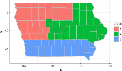The assumed group structure in Iowa is shown in Figure 1 with three groups. The three groups are aggregated based on the districts available on https://www.nass.usda.gov/Charts_and_Maps/Crops_County/boundary_maps/indexpdf.php

Figure 1. Group information.

We consider three different sets of parameters.

• Case I: ${\mathit{\beta }}_i=(0.5,0.5{)}^{\mathrm{T}}$if $i\in {\mathcal{G}}_1$, ${\mathit{\beta }}_i=(2,2{)}^{\mathrm{T}}$ if $i\in {\mathcal{G}}_2$ and ${\mathit{\beta }}_i=(3.5,3.5{)}^{\mathrm{T}}$ if $i\in {\mathcal{G}}_3$.

• Case II: ${\mathit{\beta }}_i=(0.5,0.5{)}^{\mathrm{T}}$if $i\in {\mathcal{G}}_1$, ${\mathit{\beta }}_i=(1.5,1.5{)}^{\mathrm{T}}$ if $i\in {\mathcal{G}}_2$ and ${\mathit{\beta }}_i=(2.5,2.5{)}^{\mathrm{T}}$ if $i\in {\mathcal{G}}_3$.

• Case III: ${\mathit{\beta }}_i=(0.5,0.5{)}^{\mathrm{T}}$if $i\in {\mathcal{G}}_1$, ${\mathit{\beta }}_i=(1,1{)}^{\mathrm{T}}$ if $i\in {\mathcal{G}}_2$ and ${\mathit{\beta }}_i=(1.5,1.5{)}^{\mathrm{T}}$ if $i\in {\mathcal{G}}_3$.

For each set of parameters, ${\sigma }_{ϵ}=0.5,1,2$ are considered and ${ϵ}_{ih}\stackrel{iid}{\sim }N(0,{\sigma }_{ϵ}^2)$. For the proposed estimator, we consider both the equal weight ($c_{ij}=1$) and the spatial weight selected based on the modified BIC. Different estimators are compared by $\mathrm{R}\mathrm{M}\mathrm{S}\mathrm{E}\left({\hat{\overline{Y}}}_i^E\right)=\sqrt{\frac{1}{B}\sum _{b=1}^B{\left({\hat{\overline{Y}}}_{i\left(b\right)}^{\mathrm{E}}-{\overline{Y}}_{i\left(b\right)}\right)}^2},$

where ${\hat{\overline{Y}}}_{i\left(b\right)}^{\mathrm{E}}$ is the estimated population mean in area i and ${\overline{Y}}_{i\left(b\right)}$ is the population mean in the bth simulation, ‘E’ is the index of estimators which can be 1 or 2, and B=100. All the simulations are implemented in the Owens clusters of Ohio supercomputer centre (Ohio Supercomputer Center, 2016).

Figures 2, 3 and 4 show the results of the three sets of parameters when the sampling rate is 1% for 99 areas. ‘direct’ represents the direct estimator, which is the sample mean for simple random sampling. ‘BHF’ is calculated using the sae package provided in (1(1) $y_{ih}={\mathit{x}}_{ih}^{\mathrm{T}}\mathit{\beta }+v_i+{ϵ}_{ih},$(1) ). Under two different weights, we consider two small area estimators described in Section 2.3. ‘equal1’ and ‘sp1’ represent the estimator in (8(8) ${\hat{\overline{Y}}}_i^{\left(1\right)}={\overline{\mathit{X}}}_i^{\mathrm{T}}{\hat{\mathit{\beta }}}_i+{\hat{v}}_i,$(8) ) with equal weights and spatial weights, respectively. ‘equal2’ and ‘sp2’ represent the estimator in (9(9) $\begin{array}{rl}{\hat{\overline{Y}}}_i^{\left(2\right)}& =\frac{1}{N_i}\left(\sum _{h\in A_i}{y}_{ih}+\sum _{h\in C_i}{\hat{y}}_{ih}\right)\\ & =f_i{\overline{y}}_i+{\left({\overline{\mathit{X}}}_i-f_i\overline{{\mathit{x}}_i}\right)}^{\mathrm{T}}{\hat{\mathit{\beta }}}_i+\left(1-f_i\right){\hat{v}}_i,\end{array}$(9) ) with equal weights and spatial weights, respectively.

Figure 2. RMSE under Case I.

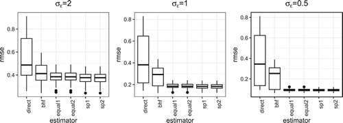
Figure 3. RMSE under Case II.

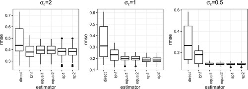
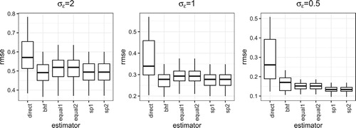
Figure 4. RMSE under Case III.

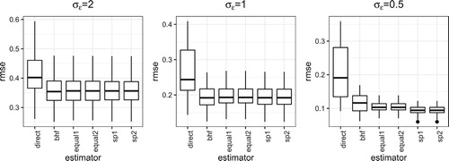
When ${\sigma }_{ϵ}$ is large, the proposed new estimator has the similar performance to the BHF estimator when the group difference is small. As ${\sigma }_{ϵ}$ becomes smaller, the performance gain of the proposed new estimator is better than the classical BHF estimator. Besides that, the estimator with spatial weights performs better than the estimator with equal weights. Since the sampling rate is small, thus $f_i$ is small, there is not much difference between the two estimators in (8(8) ${\hat{\overline{Y}}}_i^{\left(1\right)}={\overline{\mathit{X}}}_i^{\mathrm{T}}{\hat{\mathit{\beta }}}_i+{\hat{v}}_i,$(8) ) and (9(9) $\begin{array}{rl}{\hat{\overline{Y}}}_i^{\left(2\right)}& =\frac{1}{N_i}\left(\sum _{h\in A_i}{y}_{ih}+\sum _{h\in C_i}{\hat{y}}_{ih}\right)\\ & =f_i{\overline{y}}_i+{\left({\overline{\mathit{X}}}_i-f_i\overline{{\mathit{x}}_i}\right)}^{\mathrm{T}}{\hat{\mathit{\beta }}}_i+\left(1-f_i\right){\hat{v}}_i,\end{array}$(9) ).

Figures 5, 6 and 7 show the results when the sampling rate is 0.5%. When the sample sizes become smaller and ${\sigma }_{ϵ}$ is large, the proposed estimator with equal weights can be worse than the BHF estimator. But the estimator based on spatial weights is still comparable. Similarly to the case with sampling rate 1%, the proposed estimator performs better when the group difference is large or the value of ${\sigma }_{ϵ}$ is small.

Figure 5. RMSE under Case I.

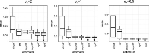
Figure 6. RMSE under Case II.

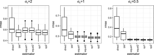
Figure 7. RMSE under Case III.

4. Real data analysis

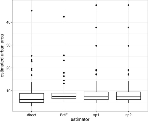
In this section, we apply the proposed method to the NRI Iowa urban data in 2015. The auxiliary information used is based on the Landsat data (Li et al., 2018). The Landsat data is matched to the segment level data in the NRI based on segments' locations. The number of segments per county is from 7 to 56. We try different starting values and select the best one with spatial weights. After finding the estimated group structure, we refit the model with known group structure and find the regression coefficients in all groups and then obtain the estimates in each county. Figure 8 shows the estimated group map. And Figure 9 shows the estimated population mean of urban in each county with a comparison with the sample mean and the BHF estimator. The proposed estimates are close to the estimates based on BHF, but with larger variations among different counties due to the fact that more than one groups are used in the estimates.

Figure 8. Estimated group structure.

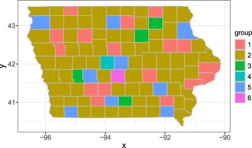
Figure 9. Estimated population mean of urban in each county.

5. Summary and conclusion

In this article, we propose a new unit level small area estimator based on a penalised regression approach. In the new estimator, we can find subgroups of areas and also borrow information from both auxiliary information and areas. Besides that, spatial information is also used in the algorithm. We use simulation studies to compare the performance of the new estimator to traditional estimators under several simulation settings, which show that the proposed estimator can improve the estimates.

Variance estimator is also important in survey sampling. A future work is to develop the variance estimator for the proposed new estimator. Another potential future work is to find subgroups for both regression coefficients and random effects together.

Disclosure statement

No potential conflict of interest was reported by the authors.

Additional information

Funding

This research was supported in part by the Natural Resources Conservation Service of the U.S. Department of Agriculture.

Notes on contributors

Xin Wang

Xin Wang is currently an Assistant professor in Department of Statistics at Miami University. Her research interests are spatial data analysis, Bayesian statistics, clustering, convergence rates of MCMC algorithms and survey sampling.

Zhengyuan Zhu

Zhengyuan Zhu is currently a Professor in Department of Statistics at Iowa State University, director of Center for Survey Statistics & Methodology. His research interests include spatial statistics, survey statistics, time series analysis, and multivariate analysis.

Appendix

In this appendix, details of partial derivative are provided. $\begin{array}{rl}\frac{\mathrm{\partial }l}{\mathrm{\partial }{\sigma }_v^2}& =-\frac{1}{2}\sum _{i=1}^m\frac{1}{n_i}tr\left({\mathrm{\Sigma }}_i^{-1}\frac{\mathrm{\partial }{\mathrm{\Sigma }}_i}{\mathrm{\partial }{\sigma }_v^2}\right)\\ & -\frac{1}{2}\sum _{i=1}^m\frac{1}{n_i}{\left({\mathit{y}}_i-{\mathit{x}}_i^{\mathrm{T}}{\mathit{\beta }}_i\right)}^{\mathrm{T}}\frac{\mathrm{\partial }{\mathrm{\Sigma }}_i^{-1}}{\mathrm{\partial }{\sigma }_v^2}\left({\mathit{y}}_i-{\mathit{x}}_i^{\mathrm{T}}{\mathit{\beta }}_i\right),\\ \frac{\mathrm{\partial }l}{\mathrm{\partial }{\sigma }_{ϵ}^2}& =-\frac{1}{2}\sum _{i=1}^m\frac{1}{n_i}tr\left({\mathrm{\Sigma }}_i^{-1}\frac{\mathrm{\partial }{\mathrm{\Sigma }}_i}{\mathrm{\partial }{\sigma }_{ϵ}^2}\right)\\ & -\frac{1}{2}\sum _{i=1}^m\frac{1}{n_i}{\left({\mathit{y}}_i-{\mathit{x}}_i^{\mathrm{T}}{\mathit{\beta }}_i\right)}^{\mathrm{T}}\frac{\mathrm{\partial }{\mathrm{\Sigma }}_i^{-1}}{\mathrm{\partial }{\sigma }_{ϵ}^2}\left({\mathit{y}}_i-{\mathit{x}}_i^{\mathrm{T}}{\mathit{\beta }}_i\right),\end{array}$ where $\begin{array}{rl}\frac{\mathrm{\partial }{\mathrm{\Sigma }}_i}{\mathrm{\partial }{\sigma }_v^2}& ={\mathbf{1}}_{n_i}{\mathbf{1}}_{n_i}^{\mathrm{T}},\frac{\mathrm{\partial }{\mathrm{\Sigma }}_i}{\mathrm{\partial }{\sigma }_{ϵ}^2}={\mathit{I}}_{n_i},\\ \frac{\mathrm{\partial }{\mathrm{\Sigma }}_i^{-1}}{\mathrm{\partial }{\sigma }_v^2}& =-\frac{1}{{\left({\sigma }_{ϵ}^2+n_i{\sigma }_v^2\right)}^2}{\mathbf{1}}_{n_i}{\mathbf{1}}_{n_i}^{\mathrm{T}}\\ \frac{{\mathrm{\Sigma }}_i^{-1}}{\mathrm{\partial }{\sigma }_{ϵ}^2}& =\frac{1}{{\left({\sigma }_{ϵ}^2\right)}^2}\left[\frac{{\sigma }_v^2\left(2{\sigma }_{ϵ}^2+n_i{\sigma }_v^2\right)}{{\left({\sigma }_{ϵ}^2+n_i{\sigma }_v^2\right)}^2}{\mathbf{1}}_{n_i}{\mathbf{1}}_{n_i}^{\mathrm{T}}-{\mathit{I}}_{n_i}\right].\end{array}$$\mathcal{I}$ can be written as $\mathcal{I}=\left(\begin{array}{cc}{\mathcal{I}}_{11}& {\mathcal{I}}_{12}\\ {\mathcal{I}}_{21}& {\mathcal{I}}_{22}\end{array}\right),$ where $\begin{array}{rl}{\mathcal{I}}_{11}& =\frac{1}{2}\sum _{i=1}^m\frac{1}{n_i}tr\left({\mathrm{\Sigma }}_i^{-1}\frac{\mathrm{\partial }{\mathrm{\Sigma }}_i}{\mathrm{\partial }{\sigma }_v^2}{\mathrm{\Sigma }}_i^{-1}\frac{\mathrm{\partial }{\mathrm{\Sigma }}_i}{\mathrm{\partial }{\sigma }_v^2}\right)\\ & =\frac{1}{2}\sum _{i=1}^m\frac{n_i}{{\left({\sigma }_{ϵ}^2+n_i{\sigma }_v^2\right)}^2},\\ {\mathcal{I}}_{12}& ={\mathcal{I}}_{21}=\frac{1}{2}\sum _{i=1}^m\frac{1}{n_i}tr\left({\mathrm{\Sigma }}_i^{-1}\frac{\mathrm{\partial }{\mathrm{\Sigma }}_i}{\mathrm{\partial }{\sigma }_v^2}{\mathrm{\Sigma }}_i^{-1}\frac{\mathrm{\partial }{\mathrm{\Sigma }}_i}{\mathrm{\partial }{\sigma }_{ϵ}^2}\right)\\ & =\frac{1}{2}\sum _{i=1}^m\frac{1}{{\left({\sigma }_{ϵ}^2+n_i{\sigma }_v^2\right)}^2},\\ {\mathcal{I}}_{22}& =\frac{1}{2}\sum _{i=1}^m\frac{1}{n_i}tr\left({\mathrm{\Sigma }}_i^{-1}\frac{\mathrm{\partial }{\mathrm{\Sigma }}_i}{\mathrm{\partial }{\sigma }_{ϵ}^2}{\mathrm{\Sigma }}_i^{-1}\frac{\mathrm{\partial }{\mathrm{\Sigma }}_i}{\mathrm{\partial }{\sigma }_{ϵ}^2}\right)\\ & =\frac{1}{2{\left({\sigma }_{ϵ}^2\right)}^2}\sum _{i=1}^m\left[1-\frac{{\sigma }_v^2\left(2{\sigma }_{ϵ}^2+n_i{\sigma }_v^2\right)}{{\left({\sigma }_{ϵ}^2+n_i{\sigma }_v^2\right)}^2}\right].\end{array}$

References

- Battese, G. E., Harter, R. M., & Fuller, W. A. (1988). An error-components model for prediction of county crop areas using survey and satellite data. Journal of the American Statistical Association, 83(401), 28–36.
- Boyd, S., Parikh, N., Chu, E., Peleato, B., & Eckstein, J. (2011). Distributed optimization and statistical learning via the alternating direction method of multipliers. Foundations and Trends in Machine Learning, 3(1), 1–122.
- Fan, J., & Li, R. (2001). Variable selection via nonconcave penalized likelihood and its oracle properties. Journal of the American statistical Association, 96(456), 1348–1360.
- Li, X., Zhou, Y., Zhu, Z., Liang, L., Yu, B., & Cao, W. (2018). Mapping annual urban dynamics (1985–2015) using time series of Landsat data. Remote Sensing of Environment, 216, 674–683.
- Ma, S., & Huang, J. (2017). A concave pairwise fusion approach to subgroup analysis. Journal of the American Statistical Association, 112(517), 410–423.
- Ma, S., Huang, J., & Zhang, Z (2016). Exploration of heterogeneous treatment effects via concave fusion. arXiv preprint arXiv:1607.03717.
- Molina, I., & Marhuenda, Y. (2015). sae: An R package for small area estimation. The R Journal, 7(1), 81–98.
- Nusser, S. M., & Goebel, J. J. (1997). The national resources inventory: A long-term multi-resource monitoring programme. Environmental and Ecological Statistics, 4(3), 181–204.
- Ohio Supercomputer Center (2016). Owens supercomputer. http://osc.edu/ark:/19495/hpc6h5b1.
- Pfeffermann, D. (2013). New important developments in small area estimation. Statistical Science, 28(1), 40–68.
- Rao, J. N., & Molina, I. (2015). Small area estimation. Hoboken, New Jersey: John Wiley & Sons.
- Wang, H., Li, R., & Tsai, C.-L. (2007). Tuning parameter selectors for the smoothly clipped absolute deviation method. Biometrika, 94(3), 553–568.
- Wang, X., Zhu, Z., & Zhang, H. H (2019). Spatial automatic subgroup analysis for areal data with repeated measures. arXiv preprint arXiv:11906.01853.
- Zhang, C.-H. (2010). Nearly unbiased variable selection under minimax concave penalty. The Annals of statistics, 38(2), 894–942.
- Zhu, R., Zou, G., Liang, H., & Zhu, L. (2016). Penalized weighted least squares to small area estimation. Scandinavian Journal of Statistics, 43(3), 736–756.