Generalised variance functions for longitudinal survey data

ABSTRACT

In this research, we propose longitudinal generalised variance functions (LGVFs) to produce convenient estimates of variances by incorporating time effect into modelling. Asymptotic properties of some certain type of estimators are investigated. Simulation studies and implementation of the proposed methods to Current Population Survey (CPS) data show that LGVFs work well in producing standard error estimates.

KEYWORDS:

• CPS
• design effect
• generalised variance function
• longitudinal generalised variance function
• simulation

1. Introduction

In many large-scale sample surveys such as the CPS or the Canadian Labour Force Survey (CLFS), thousands of estimates need to be reported. Calculating standard error for each published estimator involves a large amount of work. In addition, standard error estimates that are not provided by public-use files may also be needed. In a generalised variance function (GVF), we first estimate variances for totals of a group of variables by using balanced repeated replication (BRR), Taylor Series Linearisation (TSL) or other methods. Interested readers in variance estimation of a sample survey can refer to Cohen (1979), Burt and Cohen (1984), Rao and Wu (1988), Rao (1988), and Wolter (2007). Next, we postulate a regression model relating the variance with the estimated totals and derive a fitted regression line for the purpose of predicting the standard errors of potential survey statistics. The GVF method saves a lot of time to produce the government reports.

Johnson and King (1987) studied GVF estimators using a national survey of reading ability among young adults and found out that one way to markedly improve upon the GVF model is to use the prior information about the design effect (deff) of an individual estimator. Valliant (1987) proved that the GVF model produces consistent estimates of the variance for a certain class of superpopulation models. He also mentioned that if the deffs for the group of estimated totals are similar, the GVF variances were often more stable than the direct estimate, as they smooth out some of the variability from variable to variable.

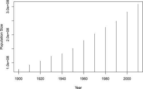
Many current surveys follow the same households at regular time intervals. GVF could be applied to analyse longitudinal data by treating population total as a constant over years. However, as Figure 1 shows, the Census population from 1900 to 2010 exhibits a linear or slight exponential growth trend. Thompson (2015) discussed approaches to incorporate complex designs in longitudinal data inference, as well as the complications introduced by time-in-sample effects. On the other hand, separate GVFs for each year sounds no longer a wise choice as we have longitudinal data. Shook-Sa, Heller, Williams, Couzens, and Berzofsky (2013) mentioned, separate GVFs are currently needed for each year in National Crime Victimization Survey (NCVS), which makes it difficult to manage the analysis. All these request a new method that can produce a convenient formula to estimate the standard errors for longitudinal data. The fitted longitudinal model is expected to be used to predict standard errors of interested variables in the future without estimating GVF parameters.

Figure 1. U.S. population from 1900 to 2010.

In this research, we propose longitudinal generalised variance functions (LGVFs) by incorporating time effect into modelling. In Section 2, we review the GVF model. In Section 3, we set up a framework, propose LGVFs and derive asymptotic properties of the proposed estimators. Section 4 gives simulation studies and implementation of LGVFs with CPS data. Section 5 gives the conclusion of the research.

2. Generalised variance function model

In this section, we briefly review the GVF models. More detailed description can be found in textbooks from Wolter (2007) and Lohr (2010).

Let $\hat{T}$ be a survey statistic, for example, the estimated number of persons employed. Let $\hat{p}$ be an estimated proportion of employment, with $\hat{p}=\hat{T}/M$, where M is the population total from the U.S. Census Bureau. Let d be the design effect of $\hat{p}$ and m be the sample size. We have $\text{var}\left(\hat{p}\right)=d\times p(1-p)/m.$ Define relative variance (relvar) of $\hat{p}$ as $\text{relvar}\left(\hat{p}\right)=\frac{\text{var}\left(\hat{p}\right)}{\left[E\right(\hat{p}){]}^2}=a+\frac{b}{E\left(\hat{T}\right)},$ where $a=-d/m$ and $b=Md/m$. Let υ be the estimate of relvar of $\hat{p}$, i.e., $\upsilon =\widehat{\text{var}}\left(\hat{p}\right)/{\hat{p}}^2$. Postulate a regression model relating a set of ${\upsilon }_i$ to ${\hat{T}}_i,i=1,2,\dots ,m$ by ${\upsilon }_i=a+b/{\hat{T}}_i$. Let $\hat{a}$ and $\hat{b}$ be the regression estimates of a and b. The GVF relative variance is predicted by the fitted regression function $\hat{a}+\hat{b}/{\hat{T}}_i$. A GVF estimate for $\text{var}\left(\hat{T}\right)$ is given by the following function: (1) $\widehat{\text{var}}\left(\hat{T}\right)=\hat{a}{\hat{T}}^2+\hat{b}\hat{T}.$(1)

3. Longitudinal generalised variance functions

GVF has been widely used for a long time by many large-scale surveys because of the advantages of time saving and stability of the estimators. For example, it has been used by the CPS since 1947 (U.S. Census Bureau, 2006). In this section, we introduce the framework of our research and propose longitudinal generalised variance functions (LGVFs) by incorporating time effects. Properties of certain type of estimators are investigated.

3.1. Framework

Much of the notation in this section follows from Valliant (1987). The main difference is that we have added index $t,t=1,2,\dots ,\tau$ for time periods 1 to τ. In a stratified two-stage cluster sampling, we define h as the index for stratum, i as the index for primary sampling unit (psu), and j as the index for secondary sampling units (ssu) within the psu. At the psu level, let $N_t$ be the number of psus in the population at time t, $N_{th}$ be the number of psus in stratum h at time t, so that $N_t=\sum _{h=1}^H{N}_{th}$. At the ssu level, let $M_{thi}$ be the number of ssus in psu i within stratum h at time t, so that the total number of units in stratum h at time t is $M_{th}=\sum _{i=1}^{N_h}{M}_{thi}$, and the total number of ssus in the population at time t is $M_t=\sum _{h=1}^H{M}_{th}$.

Accordingly, at time t, let $n_t$ be the number of psus in the sample. Let $n_t=\sum _{h=1}^H{n}_{th}$, where $n_{th}$ is the number of psus in the sample within stratum h. Assume that $n_t=n$ for $t=1,2,\dots ,\tau$. Let $m_{thi}$ be the number of elements in the sample from ith psu within stratum h. As a result, $m_{th}=\sum _{i=1}^{n_h}{m}_{thi}$, and the total number of units in a sample over all strata $m_t=\sum _{h=1}^H{m}_{th}$. At time t, let ${\mathcal{S}}_{th}$ be the set of sampled psu in stratum h, ${\mathcal{R}}_{th}$ be the set of nonsampled psu in stratum h, and ${\mathcal{S}}_{thi}$ and ${\mathcal{R}}_{thi}$ be the set of sampled and nonsampled units within psu i in stratum h.

Using a combined inference framework, assume a random variable $y_{thij}$ is associated with each unit in the population at time t. The finite population total at time t is $T_t=\sum _{h=1}^H\sum _{i=1}^{N_{ht}}\sum _{j=1}^{M_{thi}}{y}_{thij}$. A general type of the estimator $T_t$ can be written as (2) ${\hat{T}}_t=\sum _h\sum _{i\in {\mathcal{S}}_{th}}{\gamma }_{thi}{\hat{T}}_{thi},$(2) where ${\gamma }_{thi}$ is the coefficient, ${\overline{y}}_{thi}=\sum _{j\in {\mathcal{S}}_{thi}}{y}_{thij}/m_{thi}$ and ${\hat{T}}_{thi}=M_{thi}{\overline{y}}_{thi}$, which estimates $T_{thi}=\sum _{j=1}^{M_{thi}}{y}_{thij}$. For example, the Horvitz–Thompson estimator when psus are selected with probabilities proportional to $M_{thi}$, and an equal probability sample is selected within each sampled psu at time t can be written as follows: (3) ${\hat{T}}_{t,HT}=\sum _h\sum _{i\in {\mathcal{S}}_{th}}\left[M_{th}\right(n_{th}{M}_{thi}{)}^{-1}{\hat{T}}_{thi}],$(3) where ${\gamma }_{thi}=M_{th}(n_{th}{M}_{thi}{)}^{-1}$.

The following model assumptions can be applied for prediction purposes: (4) $\begin{array}{rl}E\left(y_{thij}\right)& ={\mu }_{th}\\ \text{cov}(y_{thij},y_{t{h}^{\mathrm{\prime }}{i}^{\mathrm{\prime }}{j}^{\mathrm{\prime }}})& =\left\{\begin{array}{ll}{\sigma }_{thi}^2& \text{if }h=h^{\mathrm{\prime }},i=i^{\mathrm{\prime }},j=j^{\mathrm{\prime }}\\ {\rho }_{thi}{\sigma }_{thi}^2& \text{if }h=h^{\mathrm{\prime }},i=i^{\mathrm{\prime }},j\ne j^{\mathrm{\prime }}\\ 0& \text{otherwise}\end{array}\right.\end{array}$(4) Similar formulations can be found from Scott and Smith (1969), Royall (1976, 1986), and Burdick and Sielken (1979). We can also apply more complex models such as the one in Cook and Pocock (1983), time series models, or stochastic models. The general variance estimator of $\text{var}\left({\hat{T}}_t\right)$ to be studied is based on the one proposed by Royall (1986): (5) $s_{{\hat{T}}_t}^2=\sum _h{n}_{th}(n_{th}-1{)}^{-1}\sum _{{\mathcal{S}}_{th}}{\gamma }_{thi}^2{r}_{thi}^2,$(5) where $r_{thi}={\hat{T}}_{thi}-\left(\sum _{{\mathcal{S}}_{th}}{\gamma }_{thj}{\hat{T}}_{thj}/M_{th}\right)M_{thi}$, and ${\gamma }_{thi}$ is defined in Equation (2(2) ${\hat{T}}_t=\sum _h\sum _{i\in {\mathcal{S}}_{th}}{\gamma }_{thi}{\hat{T}}_{thi},$(2) ).

Let $k_{thi}=[1+(m_{thi}-1\left){\rho }_{thi}\right]/m_{thi}$. Under the condition that ${\sigma }_{thi}^2={\sigma }_{th}^2={\alpha }_{1th}{\mu }_{th}+{\alpha }_{2th}{\mu }_{th}^2$, we can show that (6) $\begin{array}{rl}& \text{relvar}\left({\hat{T}}_t\right)\\ & \approx \sum _h{\pi }_{th}^2{\alpha }_{2th}{M}_{th}^{-2}\sum _{{\mathcal{S}}_{th}}{\gamma }_{thi}^2{k}_{thi}{M}_{thi}^2\\ & +\left[\sum _h{\pi }_{th}{\alpha }_{1th}{M}_{th}^{-2}\sum _{{\mathcal{S}}_{th}}{\gamma }_{thi}^2{k}_{thi}{M}_{thi}^2\right]/E\left({\hat{T}}_t\right)\\ & =a_t+b_t/E\left({\hat{T}}_t\right),\end{array}$(6) where ${\pi }_{th}=E\left({\hat{T}}_{th}\right)/E\left({\hat{T}}_t\right)$.

3.2. The time effect model

In this section, we propose LGVFs by incorporating time effects. Let V be the number of variables for GVF and LGVF calculation. Let τ be the number of time periods we consider for LGVF. Let $\mathit{\theta }=(a,b{)}^{\mathrm{\prime }}$ be the LGVF parameters we want to estimate. The V variables together with τ time periods provide $V\tau$ observations for regression parameters a and b estimation. Let time effect $e_t=M_t/\overline{M}$, where $\overline{M}=M_1+M_2+\cdots +M_{\tau }$. Let $a_{tv}=-d_{tv}/m$, and $b_{tv}=\overline{M}{d}_{tv}/m$. By Equation (1(1) $\widehat{\text{var}}\left(\hat{T}\right)=\hat{a}{\hat{T}}^2+\hat{b}\hat{T}.$(1) ), $\begin{array}{rl}\widehat{\text{var}}\left({\hat{T}}_{tv}\right)& =\frac{-d_{tv}}{m_t}{\hat{T}}^2+\frac{M_t{d}_{tv}}{m}{\hat{T}}_{tv}\\ & =\frac{-d_{tv}}{m_t}{\hat{T}}^2+\frac{M_t\overline{M}{d}_{tv}}{\overline{M}m}{\hat{T}}_{tv}\\ & =a_{tv}{\hat{T}}_{tv}^2+e_t{b}_{tv}{\hat{T}}_{tv}.\end{array}$ As in GVF, we define a set of relative variances ${\upsilon }_{tv}$ for $t=1,2,\dots ,\tau$ and $v=1,2,\dots ,V$. We now have (7) ${\upsilon }_{tv}=a_{tv}+b_{tv}\cdot \frac{e_t}{{\hat{T}}_{tv}}.$(7) Let ${\mathit{\upsilon }}_t=({\upsilon }_{t1},v_{t2},\dots ,{\upsilon }_{tV}{)}^{\mathrm{\prime }}$, $\mathit{\upsilon }=({\mathit{\upsilon }}_1^{\mathrm{\prime }},\dots ,{\mathit{\upsilon }}_{\tau }^{\mathrm{\prime }}{)}^{\mathrm{\prime }}$, ${\mathit{ϵ}}_t=({ϵ}_{t1},\dots ,{ϵ}_{tV}{)}^{\mathrm{\prime }}$, and $\mathit{ϵ}=({\mathit{ϵ}}_1^{\mathrm{\prime }},\dots ,{\mathit{ϵ}}_{\tau }^{\mathrm{\prime }}{)}^{\mathrm{\prime }}$. Now define ${\mathbf{X}}_t$ as the $V\times 2$ design matrix for time t with the first column 1s and second column $(e_t/{\hat{T}}_{t1},e_t/{\hat{T}}_{t2},\dots ,e_t/{\hat{T}}_{tV}{)}^{\mathrm{\prime }}$. Let $\mathbf{X}$ be the design matrix with $\mathbf{X}=({\mathbf{X}}_1^{\mathrm{\prime }},\dots ,{\mathbf{X}}_{\tau }^{\mathrm{\prime }}{)}^{\mathrm{\prime }}$. Under the condition that $a_{tv}=a_t=a$ and $b_{tv}=b_t=b$ for $t=1,2,\dots ,\tau$, $v=1,2,\dots ,V$, time effect model (7(7) ${\upsilon }_{tv}=a_{tv}+b_{tv}\cdot \frac{e_t}{{\hat{T}}_{tv}}.$(7) ) can be written in the matrix form as follows: (8) $\mathit{\upsilon }=\mathbf{X}\mathit{\theta }+\mathit{ϵ}.$(8) The weighted least square estimators of $\mathit{\theta }$ is $\hat{\mathit{\theta }}=({\mathbf{X}}^{\mathrm{\prime }}\mathbf{W}\mathbf{X}{)}^{-1}{\mathbf{X}}^{\mathrm{\prime }}\mathbf{W}\mathit{\upsilon }$, where $w_{tv}$ is the weight associated with variable v at time t, and $\mathbf{W}$ is a $V\tau \times V\tau$ matrix with the diagonal element $w_{tv}$. $w_{tv}$ is usually chosen as the reciprocal of variance of ${\upsilon }_{tv}$ when they are known. Otherwise, we can approximate the weight by reciprocal of squared ${\upsilon }_{tv}$.

Consider data pairs $({\upsilon }_{tv},{\hat{T}}_{tv})$ for $t=1,2,\dots ,\tau$, $v=1,2,\dots ,V$. We can derive the following estimators for a and b: (9) $\hat{b}=\frac{\sum _{t=1}^{\tau }\sum _{v=1}^V{\upsilon }_{tv}[e_t{\hat{T}}_{tv}^{-1}-{\overline{T}}_{-}]/w_{tv}}{\sum _{t=1}^{\tau }\sum _{v=1}^V[e_t{\hat{T}}_{tv}^{-1}-{\overline{T}}_{-}{]}^2/w_{tv}}={\hat{S}}_1/{\hat{S}}_2$(9) and (10) $\hat{a}=\overline{\upsilon }-\hat{b}{\overline{T}}_{-},$(10) where ${\overline{T}}_{-}=\sum _{t,v}(e_t^{-1}{\hat{T}}_{tv}{w}_{tv}{)}^{-1}/\sum _{t,v}{w}_{tv}^{-1}$, $\overline{\upsilon }=\sum _{t,v}{\upsilon }_{tv}{w}_{tv}^{-1}/\sum _{t,v}{w}_{tv}^{-1}$, ${\hat{S}}_1=\sum _{t=1}^{\tau }\sum _{v=1}^V{\upsilon }_{tv}\left[e_t{\hat{T}}_{tv}^{-1}-{\overline{T}}_{-}\right]/w_{tv}$, and ${\hat{S}}_2=\sum _{t=1}^{\tau }\sum _{v=1}^V[e_t{\hat{T}}_{tv}^{-1}-{\overline{T}}_{-}{]}^2/w_{tv}$. The predicted relvariance of ${\hat{T}}_{tv}$ based on the estimated LGVF is (11) ${\hat{\upsilon }}_{tv}=\overline{\upsilon }+\hat{b}[e_t{\hat{T}}_{tv}^{-1}-{\overline{T}}_{-}].$(11) Note that model (8(8) $\mathit{\upsilon }=\mathbf{X}\mathit{\theta }+\mathit{ϵ}.$(8) ) only incorporate $e_t$. It doesn't specify what kind of time effect that $e_t$ has. The simplest case of $e_t$ could be $e_t=M_t/\overline{M}$, where $M_t$ is the population total from the U.S. Census Bureau without introducing any modelling. We can also incorporate linear time effect as illustrated in Figure 1 by the following example.

Example

Linear time effect LGVF.

Figure 1 shows that the U.S. population size increased dramatically with a linear trend during the years of 1990–2010. We now fit a simple linear regression model for the population size $M_t$ growth over time t as follows: (12) $M_t={\text{β}}_0+{\text{β}}_{1}t.$(12) By the fact that ${\widehat{\text{β}}}_0=\overline{M}-{\widehat{\text{β}}}_1\overline{t}$, we have ${\hat{e}}_t=\frac{{\hat{M}}_t}{\overline{M}}=\frac{\overline{M}+{\widehat{\text{β}}}_1(t-\overline{t})}{\overline{M}}=1+\frac{{\widehat{\text{β}}}_1}{\overline{M}}(t-\overline{t}).$ Replacing $e_t$ in (9(9) $\hat{b}=\frac{\sum _{t=1}^{\tau }\sum _{v=1}^V{\upsilon }_{tv}[e_t{\hat{T}}_{tv}^{-1}-{\overline{T}}_{-}]/w_{tv}}{\sum _{t=1}^{\tau }\sum _{v=1}^V[e_t{\hat{T}}_{tv}^{-1}-{\overline{T}}_{-}{]}^2/w_{tv}}={\hat{S}}_1/{\hat{S}}_2$(9) ) and (10(10) $\hat{a}=\overline{\upsilon }-\hat{b}{\overline{T}}_{-},$(10) ) by $1+{\widehat{\text{β}}}_1(t-\overline{t})/\overline{M}$, we have the LGVF estimates for linear time model (12(12) $M_t={\text{β}}_0+{\text{β}}_{1}t.$(12) ).

3.3. Properties of proposed estimators

In this section, we consider a certain type of estimators such that ${\gamma }_{thi}$ in Equation (2(2) ${\hat{T}}_t=\sum _h\sum _{i\in {\mathcal{S}}_{th}}{\gamma }_{thi}{\hat{T}}_{thi},$(2) ) is with a structure of ${\gamma }_{thi}=g_{1th}{g}_{2thi}$. For example, $g_{1th}=M_{th}/n_{th}$ for ${\hat{T}}_{HT}$ in Equation (3(3) ${\hat{T}}_{t,HT}=\sum _h\sum _{i\in {\mathcal{S}}_{th}}\left[M_{th}\right(n_{th}{M}_{thi}{)}^{-1}{\hat{T}}_{thi}],$(3) ). Under assumptions (4(4) $\begin{array}{rl}E\left(y_{thij}\right)& ={\mu }_{th}\\ \text{cov}(y_{thij},y_{t{h}^{\mathrm{\prime }}{i}^{\mathrm{\prime }}{j}^{\mathrm{\prime }}})& =\left\{\begin{array}{ll}{\sigma }_{thi}^2& \text{if }h=h^{\mathrm{\prime }},i=i^{\mathrm{\prime }},j=j^{\mathrm{\prime }}\\ {\rho }_{thi}{\sigma }_{thi}^2& \text{if }h=h^{\mathrm{\prime }},i=i^{\mathrm{\prime }},j\ne j^{\mathrm{\prime }}\\ 0& \text{otherwise}\end{array}\right.\end{array}$(4) ), given estimators with the structure of ${\gamma }_{thi}=g_{1th}{g}_{2thi}$, asymptotic properties of ${\hat{T}}_{tv}$, $s_{\widehat{T_{tv}}}^2$, and ${\hat{\upsilon }}_v$ can be derived when the number of psus in each stratum is large. Lemmas A.1–A.3 (refer to Appendix) are extensions of work by Royall (1986). Under certain conditions, Theorem 3.1 shows that ratios of relative variances and predicted relative variances from proposed LGVFs converge in probability to 1 (refer to Appendix for proof). The asymptotic normality then follows immediately.

Theorem 3.1

Under model (4(4) $\begin{array}{rl}E\left(y_{thij}\right)& ={\mu }_{th}\\ \text{cov}(y_{thij},y_{t{h}^{\mathrm{\prime }}{i}^{\mathrm{\prime }}{j}^{\mathrm{\prime }}})& =\left\{\begin{array}{ll}{\sigma }_{thi}^2& \text{if }h=h^{\mathrm{\prime }},i=i^{\mathrm{\prime }},j=j^{\mathrm{\prime }}\\ {\rho }_{thi}{\sigma }_{thi}^2& \text{if }h=h^{\mathrm{\prime }},i=i^{\mathrm{\prime }},j\ne j^{\mathrm{\prime }}\\ 0& \text{otherwise}\end{array}\right.\end{array}$(4) ), assumptions (i) to (xiii), ${\mu }_{4thi}=E[{\hat{T}}_{thi}-E({\hat{T}}_{thi}){]}^4<\mathrm{\infty },$ $a_{tv}=a_t=a,$ and $b_{tv}=b_t=b$ for $t=1,2,\dots ,\tau ,$ $v=1,2,\dots ,V,$ as $N_{th},n_{th}\to \mathrm{\infty },$ $\frac{\text{relvar}({\hat{T}}_{tv}-T_{tv})}{{\hat{\upsilon }}_v}\stackrel{p}{\to }1.$

Proof.

Proof is given in Appendix.

Theorem 3.2

Under model (4(4) $\begin{array}{rl}E\left(y_{thij}\right)& ={\mu }_{th}\\ \text{cov}(y_{thij},y_{t{h}^{\mathrm{\prime }}{i}^{\mathrm{\prime }}{j}^{\mathrm{\prime }}})& =\left\{\begin{array}{ll}{\sigma }_{thi}^2& \text{if }h=h^{\mathrm{\prime }},i=i^{\mathrm{\prime }},j=j^{\mathrm{\prime }}\\ {\rho }_{thi}{\sigma }_{thi}^2& \text{if }h=h^{\mathrm{\prime }},i=i^{\mathrm{\prime }},j\ne j^{\mathrm{\prime }}\\ 0& \text{otherwise}\end{array}\right.\end{array}$(4) ), assumptions (i) to (xiii), ${\mu }_{4thi}=E[{\hat{T}}_{thi}-E({\hat{T}}_{thi}){]}^4<\mathrm{\infty },$ $a_{tv}=a_t=a,$ and $b_{tv}=b_t=b$ for $t=1,2,\dots ,\tau ,$ $v=1,2,\dots ,V,$ as $N_{th},n_{th}\to \mathrm{\infty },$ $\frac{{\hat{T}}_{tv}-T_{tv}}{{\hat{T}}_{tv}({\hat{\upsilon }}_v{)}^{1/2}}\stackrel{d}{\to }N(0,1).$

Proof.

The proof is a straightforward extension of work by Royall (1986).

4. Implementation with CPS

In this section, we first use CPS annual social and economic supplement (ASEC) data as a population to perform simulation studies. Next, we apply the proposed methods to analyse ASEC data in conjunction with ASEC public use replicate weight file (ASECREP). The corresponding ASECREP data are merged with ASEC by the link variables $h_{seq}$ (household sequence number) and pppos (trailer portion of unique household ID) for variance estimation purpose in data application. The ASECREP data have weights for the variables according to 160 replications, which are used to calculate variances. Nineteen binary variables from the ‘Source of Income’ section are initially considered, such as self-employment or not, unemployment compensation or not, and so on. Specifically, they are finc_ws, finc_se, finc_fr, finc_uc, finc_wc, finc_ss, finc_ssi, finc_paw, finc_vet, finc_sur, finc_dis, finc_ret, finc_int, finc_div, finc_rnt, finc_ed, finc_csp, finc_fin, and finc_oi.

A person's value of a binary variable is 1 if the person had a particular characteristic, and is 0 otherwise. By examining 2009 ASEC data, the mean of deffs of the 19 variables is 3.754811, and the range of deffs is from 1.593687 to 6.329467. We removed two variables with the low deffs: finc_ss with deff of 1.593687, and finc_sur with deff of 1.809737. We also removed three variables with high deffs: finc_int with deff of 6.329467; finc_div with deff of 6.073850, and finc_fin with deff of 5.559943. The remaining 14 variables are relatively similar regarding deffs with a mean of 3.569623, and a narrower range from 2.059918 to 5.424058. These 14 binary variables are used to construct GVFs (using 2011 ASEC data) and LGVFs (using 2008 to 2010 ASEC data). In the simulation study, we removed variable finc_ws due to its very low relative variance. We restricted our analysis to the state of New Mexico when we apply ASEC and ASECREP data.

4.1. Simulation studies

We treat 2008 (2059 observations), 2009 (2188 observations), and 2010 (2108 observations) ASEC data in New Mexico as finite population. Each household was associated with an ultimate sampling unit (USU) defined for the CPS. However, the USU information is not released to public. To mimic the design, we sorted households from the smallest sequence number to the largest one within each year and combined four households as a USU according to order. This results in 205, 208, and 193 USUs, respectively. Simulation is performed with the following steps:

1. Within each year, we select n=40 (about 20% sampling rate) and n=100 (about 50% sampling rate) USUs with probabilities proportional to size (PPS) and select $m_i=4$ individuals within selected USU i with equal probability.

2. Calculate estimates for the three samples (2008, 2009 and 2010). Total for variable v at time t is estimated by the Horvitz–Thompson estimator in Equation (3(3) ${\hat{T}}_{t,HT}=\sum _h\sum _{i\in {\mathcal{S}}_{th}}\left[M_{th}\right(n_{th}{M}_{thi}{)}^{-1}{\hat{T}}_{thi}],$(3) ), denoted by ${\hat{T}}_{tv}$; variance is estimated by Equation (5(5) $s_{{\hat{T}}_t}^2=\sum _h{n}_{th}(n_{th}-1{)}^{-1}\sum _{{\mathcal{S}}_{th}}{\gamma }_{thi}^2{r}_{thi}^2,$(5) ), denoted by $s_{{\hat{T}}_{tv}}^2$; relative variance (relvar) is calculated as ${\upsilon }_{tv}=s_{{\hat{T}}_{tv}}^2/{\hat{T}}_{tv}^2$.

3. Apply time adjustment $e_t$ to estimates from step (b) using $e_t/{\hat{T}}_{tv}$, where $e_1=M_1/\overline{M}=1,978,390/1,967,487=1.0056$ (for year 2009); $e_2=M_2/\overline{M}=1,977,807/1,967,487=1.0052$ (for year 2010); and $e_3=M_3/\overline{M}=1,946,264/1,967,487=0.9892$ (for year 2008).

4. Apply regression model (7(7) ${\upsilon }_{tv}=a_{tv}+b_{tv}\cdot \frac{e_t}{{\hat{T}}_{tv}}.$(7) ) with fitting methods LGVF1 (ordinary linear regression) and LGVF2 (weighted least squares with $w_{tv}=1/{\upsilon }_{tv}^2$).

5. Record relvar calculated by using formulas (3(3) ${\hat{T}}_{t,HT}=\sum _h\sum _{i\in {\mathcal{S}}_{th}}\left[M_{th}\right(n_{th}{M}_{thi}{)}^{-1}{\hat{T}}_{thi}],$(3) ) and (5(5) $s_{{\hat{T}}_t}^2=\sum _h{n}_{th}(n_{th}-1{)}^{-1}\sum _{{\mathcal{S}}_{th}}{\gamma }_{thi}^2{r}_{thi}^2,$(5) ); record relvar calculated by using fitted values from LGVF1 and LGVF2 (LGVFs 1–2); and record standard errors of the fitted relvar by LGVFs 1–2.

6. Repeat (a)–(e) for 2000 times. For each variable, record average values of the relvar calculated by Equations (3(3) ${\hat{T}}_{t,HT}=\sum _h\sum _{i\in {\mathcal{S}}_{th}}\left[M_{th}\right(n_{th}{M}_{thi}{)}^{-1}{\hat{T}}_{thi}],$(3) ) and (5(5) $s_{{\hat{T}}_t}^2=\sum _h{n}_{th}(n_{th}-1{)}^{-1}\sum _{{\mathcal{S}}_{th}}{\gamma }_{thi}^2{r}_{thi}^2,$(5) ) (treated as true relvar); record average values of the relvar estimated by fitted values using LGVFs 1–2 (treated as estimated value of relvar); record sampling variance of relvar calculated by Equations (3(3) ${\hat{T}}_{t,HT}=\sum _h\sum _{i\in {\mathcal{S}}_{th}}\left[M_{th}\right(n_{th}{M}_{thi}{)}^{-1}{\hat{T}}_{thi}],$(3) ) and (5(5) $s_{{\hat{T}}_t}^2=\sum _h{n}_{th}(n_{th}-1{)}^{-1}\sum _{{\mathcal{S}}_{th}}{\gamma }_{thi}^2{r}_{thi}^2,$(5) ) (treated as true variance of relvar); and record average standard errors of the fitted relvar by LGVFs 1–2 (estimated variance of relvar).

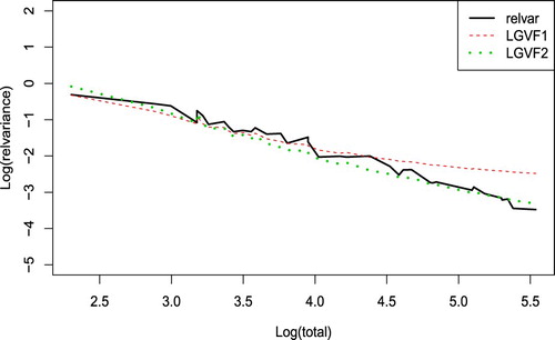
Simulation results of both cases: PPS 40 USUs and PPS 100 USUs are very close to each other, so we will only report results from the case of PPS 100 USUs. The case of PPS 100 USUs performs slightly better than the other case regarding bias and variance. This is very reasonable as Theorems 3.1 and 3.2 require large $N_{th}$ and $n_{th}$. Figure 2 is the plot of logs of relvars by Equations (3(3) ${\hat{T}}_{t,HT}=\sum _h\sum _{i\in {\mathcal{S}}_{th}}\left[M_{th}\right(n_{th}{M}_{thi}{)}^{-1}{\hat{T}}_{thi}],$(3) ) and (5(5) $s_{{\hat{T}}_t}^2=\sum _h{n}_{th}(n_{th}-1{)}^{-1}\sum _{{\mathcal{S}}_{th}}{\gamma }_{thi}^2{r}_{thi}^2,$(5) ) (solid line, treated as true values) and estimates from LGVFs 1–2 (dashed line and dotted line) plotted versus logs of population totals. From the plot, we can see that LGVF2 works very well in estimating the true relvars. LGVF1 deviates from the true value quite a bit when the population total of the variables is large.

Figure 2. Logs of estimates of relvar plotted versus logs of population totals.

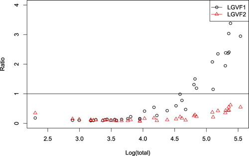
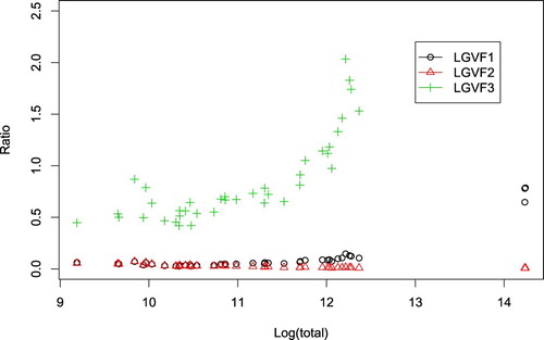
To see how precise our LGVF estimators are, we also plot the ratios of standard error estimates of relvars by LGVFs 1–2 to the standard error estimate of relvars calculated by sampling variability from simulations (see Figure 3). Ratios less than 1 indicate that an LGVF is more precise than the sampling variability by simulations. LGVF2 is doing perfect in estimating the variance of relvar with none of the ratios greater than 1. While not surprisingly, LGVF1 has large variance when population total of the variable is large. But LGVF1 is also doing Okay.

Figure 3. Ratio of the SEs (LGVF1–LGVF2/relvar) versus log (totals).

We also investigated the histograms of the binary variables to see how Theorem 3.2 works. We observe that asymptotic normality reveals well with high proportion variable such as finc_se (with a total of 211). While for small total variable such as finc_dis with a total of only 10, the histogram is highly skewed to the left as samples with small totals are frequently selected.

4.2. Data analysis: apply LGVF to the full 2008–2010 data

In this section, we apply our methods to the full data set, which we used as population in simulation studies. The 14 binary variables used to construct GVFs and LGVFs are from the ‘Source of Income’ section of ASEC without the two lowest and three highest deff scores as we discussed in Section 4. In data analysis, variance is calculated by using replicate weights and a formula provided by ASECPEP user's manual (U.S. Census Bureau, 2009): $\text{var}\left({\hat{p}}_i\right)=4\ast \sum _{i=1}^{160}({\hat{p}}_i-{\hat{p}}_0{)}^2/160$, where ${\hat{p}}_0$ is calculated using weights ‘PWWGT0’ for full data, and ${\hat{p}}_i,i=1,2,\dots ,160$ are calculated by using the 160 replicate weights ‘PWWGT1’ to ‘PWWGT160’. This is essentially the empirical variance adjusted by a factor of 4. The estimated totals ${\hat{T}}_{tv}$ are calculated by using full data weights ‘PWWGT0’. We then postulate a regression function on the relative variances and the adjusted estimated totals $e_t/{\hat{T}}_{tv}$ to derive the estimates of the regression parameters a and b.

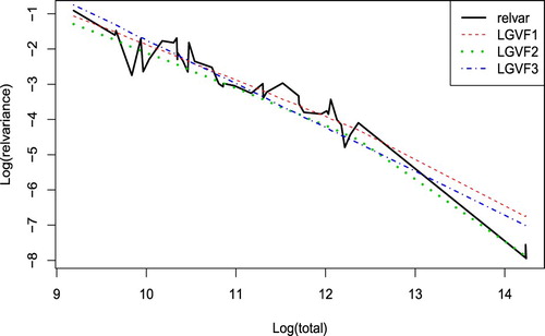
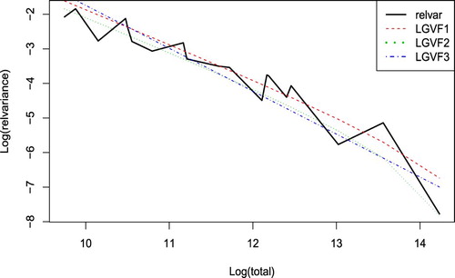
Regression fitting methods, LGVF1: ordinary linear regression, LGVF2: weighted least squares with $w_{tv}=1/{\upsilon }_{tv}^2$, and LGVF3: data after log transformation on both y and x are applied. Figure 4 is the plot of logs of estimates of relative variances and the estimates from the LGVFs 1–3 plotted versus logs of population totals. From the plot, we can see that LGVF2 (dotted line) seems to mimic the relative variances most closely. LGVF1 (dashed line) and LGVF3 (dash-dotted line) also work fine, with the tail a little off from the black line.

Figure 4. Logs of estimates of relvar plotted versus logs of population totals.

We also plot the ratios of standard error estimates of relative variances by LGVFs 1–3 to the standard error estimate of relative variance by using replicate weights to see how precise the proposed LGVF estimators are. Ratios less than 1 indicate that an LGVF is more precise than υ. LGVF1 and LGVF2 are both precise with none of the ratios greater than 1. The variance of relvar from some variables estimated by using LGVF3 is less precise than the variance estimated using replicate weights, but LGVF3 is also doing well (Figure 5).

Figure 5. Ratio of the SEs (LGVF1–LGVF3/relvar) versus log(totals).

Next, we use LGVF models to predict the relative variances of the year 2011 data. These relative variances can be calculated by the replicate weights as we have done before, which are treated as direct calculated relvar. Figure 6 shows the prediction are quite good, with LGVF2 performing the best.

Figure 6. Logs of predicted relvar by using LGVF1–3 plotted versus logs of population totals (11 March).

4.3. Comparison of GVF with LGVF

In this section, we do a brief comparison study of the performance of GVF and LGVF. The GVF models are constructed by the year 2011 data, while the LGVF models are built by using three years (2008–2010) of data with time adjustment. The same regression fitting methods: ordinary least squares (Method 1), weighted least squares (Method 2), and log transformations (Method 3) are applied to GVF modelling. Accordingly, they are called GVF1, GVF2, and GVF3. Fourteen variables are used to construct GVFs and LGVFs, and the remaining five variables are used for predicting. Mean-squared prediction errors are calculated as the average of the sum of the squares of the difference between predicted values and observed values.

Table 1 shows that LGVFs have smaller mean-squared prediction errors. When predicting the five remaining variables, GVFs and LGVFs do not make much difference. However, the case of predicting 19 variables in 2011 is standing out with SE of 0.003108 by LGVF2 compared to SE of 0.01781 by GVF1. It is quite exciting since this is the most common case we want to apply the LGVF methods. That is, we want to use a few years of data to build the LGVF model to make a prediction for future years. Since design effects do not change much over years, therefore, combining the variables from 2009 with the same variables from 2008 and 2010 should result in reasonable results. We also incorporated $e_t$ to adjust for time effect for a longitudinal issue. The LGVF methods, particularly LGVF2, perform very well regarding mean-squared prediction errors.

Table 1. Comparison of GVF and LGVF.

		GVF	LGVF
Predicting 5 left out variables	Method 1	0.02183022	0.01636561
(2011)	Method 2	0.02110222	0.01724829
	Method 3	0.01754491	0.01619439
Predicting 19 variables	Method 1	0.01781202	0.00898679
(2011, 14 grouping, 5 left out for GVF)	Method 2	0.01811376	0.00310806
(19 left out for LGVF)	Method 3	0.02436289	0.01057787

Notes: Numbers in the table are the square root of mean-squared predicted errors. Method 1 is ordinary least-squares fitting, Method 2 is weighted least-squares fitting, and Method 3 is log transformation on both y and x fitting.

5. Conclusions

In this research, we extended the Generalised Variance Functions (GVFs) to Longitudinal Generalised Variance Functions (LGVFs), which reduce to GVFs when data are cross-sectional. We incorporated time effect into modelling to adjust the dynamic time changes over the years. We show that ratios of relative variances and predicted relative variances from the proposed LGVFs converge in probability to 1 under certain conditions. Based on simulation studies, we would suggest using LGVF2 (the weighted least square regression fitting) to predict relative variances of the variables as it has smaller bias and variance compared to the other two methods. Data application to ASEC supplements using replicate weights provided by ASECPEP reveals similar findings. A comparison study between LGVF and GVF also show that LGVF is efficient in reducing the mean squared prediction errors. Future research may consider adopting mixed models and nonparametric smoothing methods for regression model fitting. In both mixed model and nonparametric application, we can add the prior design effect information into models. This may markedly improve our model as suggested by Johnson and King (1987).

Acknowledgements

The authors thank the referees for helpful comments and constructive suggestions to improve the manuscript.

Disclosure statement

No potential conflict of interest was reported by the authors.

Additional information

Notes on contributors

Guoyi Zhang

Dr Guoyi Zhang is an Associate Professor of the Department of Mathematics and Statistics at the University of New Mexico. His research areas are in nonparametric function estimation, statistical computing, and survey sampling.

Yang Cheng

Dr Yang Cheng is a Senior Mathematical Statistician at the Substance Abuse and Mental Health Administration. He works on the areas of sample designs, weighting structure, statistical estimation and modelling.

Yan Lu

Dr Yan Lu is an Associate Professor of the Department of Mathematics and Statistics at the University of New Mexico. Her research areas are in survey sampling and mixed Models.

Appendix

For each time period $t,t=1,2,\dots ,\tau$, the following conditions apply as $n_{th},N_{th}\to \mathrm{\infty }$ for $h=1,2,\dots ,H$.

1. $n_{th}/N_{th}\to 0,m_{thi}/{\gamma }_{thi}\to 0\text{ for }i=1,2,\dots ,N_{th}$

2. $n_{th}/n_t\to c_{1th}$

3. $N_{th}/N_t\to c_{2th}$

4. $n{g}_{1th}^2{n}_{th}/N_t^2\to c_{3th}$

5. $n_{th}^{-1}\sum _{i\in {\mathcal{S}}_{th}}{g}_{2thi}^2{D}_{1thi}\to V_{1th}$

6. $n_{th}^{-1}\sum _{i\in {\mathcal{S}}_{th}}{D}_{2thi}\to V_{2th}$

7. $(N_{th}-n_{th}{)}^{-1}\sum _{i\in {\mathcal{R}}_{th}}{D}_{3thi}\to V_{3th}$

8. $n_{th}^{-1}\sum _{i\in {\mathcal{S}}_{th}}{g}_{2thi}{D}_{4thi}\to V_{4th}$

9. $n_{th}^{-1}\sum _{i\in {\mathcal{S}}_{th}}{g}_{2thi}^2{M}_{thi}^{2l}\to c_{4th}^{\left(l\right)},l=0,1$

10. $n_{th}^{-1}\sum _{i\in {\mathcal{S}}_{th}}(m_{thi}/M_{thi}{)}^2{D}_{1thi}\to V_{5th}$

where

1. $D_{1thi}=M_{thi}^2{\sigma }_{thi}^2[1+(m_{thi}-1\left){\rho }_{thi}\right]/m_{thi}$

2. $D_{2thi}=(M_{thi}-m_{thi}){\sigma }_{thi}^2[1+(M_{thi}-m_{thi}-1\left){\rho }_{thi}\right]$

3. $D_{3thi}=M_{thi}{\sigma }_{thi}^2[1+(M_{thi}-1\left){\rho }_{thi}\right]$

4. $D_{4thi}=M_{thi}{\sigma }_{thi}^2(M_{thi}-m_{thi}){\rho }_{thi}$

and $c_{1th}$ through $c_{3th}$, $c_{4th}^{\left(l\right)}$, $V_{1th}$ through $V_{5th}$ are constants. By conditions (i)–(iii), we have $n_t/N_t\to 0$. $g_{1th}$ and $g_{2thi}$ have more specific forms related to the estimators. The above assumptions apply to each time period t. For all the time periods, the following conditions apply

1. $w_{tv}/d_{tv}\to {\omega }_v$

2. $M_t/N_t\to \overline{M}/\overline{N}$

3. $E\left({\hat{T}}_{tv}\right)/\overline{N}\to e_t{\psi }_v\to N_t/\overline{N}{\psi }_v$

where ${\hat{T}}_{tv}$ is the estimator of total for variable v at time t, ${\omega }_v$ and ${\psi }_v$ are constants.

Lemmas A.1–A.3 are extensions of work by Royall (1986).

Lemma A.1

Under model (4(4) $\begin{array}{rl}E\left(y_{thij}\right)& ={\mu }_{th}\\ \text{cov}(y_{thij},y_{t{h}^{\mathrm{\prime }}{i}^{\mathrm{\prime }}{j}^{\mathrm{\prime }}})& =\left\{\begin{array}{ll}{\sigma }_{thi}^2& \text{if }h=h^{\mathrm{\prime }},i=i^{\mathrm{\prime }},j=j^{\mathrm{\prime }}\\ {\rho }_{thi}{\sigma }_{thi}^2& \text{if }h=h^{\mathrm{\prime }},i=i^{\mathrm{\prime }},j\ne j^{\mathrm{\prime }}\\ 0& \text{otherwise}\end{array}\right.\end{array}$(4) ) and conditions (i) to (viii) in Appendix, $\mathrm{v}\mathrm{a}\mathrm{r}({\hat{T}}_t-T_t)\approx \sum _h\sum _{{\mathcal{S}}_{th}}{\gamma }_{thi}^2{D}_{1thi},$ where ${\gamma }_{thi}$ is defined in Equation (2(2) ${\hat{T}}_t=\sum _h\sum _{i\in {\mathcal{S}}_{th}}{\gamma }_{thi}{\hat{T}}_{thi},$(2) ), $D_{1thi}$ is defined in Appendix, and the symbol ≈ means ‘asymptotically equivalent to’.

Lemma A.2

Under model (4(4) $\begin{array}{rl}E\left(y_{thij}\right)& ={\mu }_{th}\\ \text{cov}(y_{thij},y_{t{h}^{\mathrm{\prime }}{i}^{\mathrm{\prime }}{j}^{\mathrm{\prime }}})& =\left\{\begin{array}{ll}{\sigma }_{thi}^2& \text{if }h=h^{\mathrm{\prime }},i=i^{\mathrm{\prime }},j=j^{\mathrm{\prime }}\\ {\rho }_{thi}{\sigma }_{thi}^2& \text{if }h=h^{\mathrm{\prime }},i=i^{\mathrm{\prime }},j\ne j^{\mathrm{\prime }}\\ 0& \text{otherwise}\end{array}\right.\end{array}$(4) ) and conditions (i) to (ix), $u_{4thi}=E\left[\right({\hat{T}}_{thi}-E\left({\hat{T}}_{thi}\right){]}^4<\mathrm{\infty },$ ${\gamma }_{thi}/M_{th}=o\left(n_{th}\right),$ and $s_{{\hat{T}}_t}^2$ as defined in Equation (5(5) $s_{{\hat{T}}_t}^2=\sum _h{n}_{th}(n_{th}-1{)}^{-1}\sum _{{\mathcal{S}}_{th}}{\gamma }_{thi}^2{r}_{thi}^2,$(5) ), we have $\text{var}({\hat{T}}_t-T_t)/s_{{\hat{T}}_t}^2\stackrel{p}{\to }1.$

Lemma A.3

Under model (4(4) $\begin{array}{rl}E\left(y_{thij}\right)& ={\mu }_{th}\\ \text{cov}(y_{thij},y_{t{h}^{\mathrm{\prime }}{i}^{\mathrm{\prime }}{j}^{\mathrm{\prime }}})& =\left\{\begin{array}{ll}{\sigma }_{thi}^2& \text{if }h=h^{\mathrm{\prime }},i=i^{\mathrm{\prime }},j=j^{\mathrm{\prime }}\\ {\rho }_{thi}{\sigma }_{thi}^2& \text{if }h=h^{\mathrm{\prime }},i=i^{\mathrm{\prime }},j\ne j^{\mathrm{\prime }}\\ 0& \text{otherwise}\end{array}\right.\end{array}$(4) ) and conditions (i) to (viii) and (x), $u_{4thi}<\mathrm{\infty }$ and the random variables ${\overline{y}}_{thi}(h=1,\dots ,H,i=1,\dots ,n_{th})$ are mutually independent at each time period t, then $\frac{{\hat{T}}_t-T_t}{s_{{\hat{T}}_t}}\stackrel{d}{\to }N(0,1).$

Proof of Theorem 3.1.

Proof of Theorem 3.1

Proof follows Valliant (1987). We first prove that $\text{relvar}({\hat{T}}_{tv}-T_{tv})$ has the same limit as ${\upsilon }_v$ for any time period t. Next, we prove that the estimated ${\hat{\upsilon }}_v$ converges to the same limit.

By Equation (6(6) $\begin{array}{rl}& \text{relvar}\left({\hat{T}}_t\right)\\ & \approx \sum _h{\pi }_{th}^2{\alpha }_{2th}{M}_{th}^{-2}\sum _{{\mathcal{S}}_{th}}{\gamma }_{thi}^2{k}_{thi}{M}_{thi}^2\\ & +\left[\sum _h{\pi }_{th}{\alpha }_{1th}{M}_{th}^{-2}\sum _{{\mathcal{S}}_{th}}{\gamma }_{thi}^2{k}_{thi}{M}_{thi}^2\right]/E\left({\hat{T}}_t\right)\\ & =a_t+b_t/E\left({\hat{T}}_t\right),\end{array}$(6) ), adding the subscript v and time t, we have $\text{relvar}({\hat{T}}_{tv}-T_{tv})\approx a_{tv}+b_{tv}/E\left({\hat{T}}_{tv}\right),$ where $a_{tv}=\sum _h({\pi }_{thv}/M_{th}{)}^2{\alpha }_{2thv}\sum _{{\mathcal{S}}_{hi}}{\gamma }_{thi}^2{k}_{thiv}{M}_{thi}^2,$ and $b_{tv}=\sum _h\left({\pi }_{thv}{\alpha }_{1thv}/M_{th}\right)\sum _{s_{hi}}{\gamma }_{thi}^2{k}_{thiv}{M}_{thi}^2.$ By the definition of ${\pi }_{thv},k_{thiv},D_{1thiv},{\gamma }_{thi}$ and the assumption that ${\sigma }_{thiv}^2={\sigma }_{thv}^2$, together with conditions (iv), (v), (xii), and (xiii), $\begin{array}{rl}{n}_t{a}_{tv}& =\sum _h\left(n_t{g}_{1th}^2{n}_{th}/N_t^2\right){\alpha }_{2thv}{\mu }_{thv}^2{N}_t^{2}E({\hat{T}}_{tv}{)}^{-2}{\sigma }_{thv}^{-2}\\ & \times \left(\sum _{{\mathcal{S}}_h}{g}_{2thi}^2{D}_{1thiv}/n_{th}\right)\\ & \to \sum _h{c}_{3th}{\alpha }_{2thv}{\mu }_{thv}^2{\psi }_v^{-2}{V}_{1thv}{\sigma }_{thv}^{-2}=A_{tv}.\end{array}$ Similarly, $\left(\frac{n_t}{N_t}\right)b_{tv}\to \sum _h{c}_{3th}{\alpha }_{1thv}{\mu }_{thv}{\psi }_v^{-1}{\sigma }_{thv}^{-2}{V}_{1thv}=B_{tv}.$ Let $a_{tv}=a_t=a$ for all t and v. $A_{tv}=A$ for some constant A. $b_{tv}=b_t=b$ for all t and v, so $B_{tv}=B_t=B$ for some constant B. Therefore, $n_t\text{relvar}({\hat{T}}_{tv}-T_{tv})\to A+\frac{B}{{\psi }_v}.$ Next we'll show that $n_t{\upsilon }_{tv}$ has the same limit. Lemma A.3 shows $\frac{{\hat{T}}_{tv}-E\left({\hat{T}}_{tv}\right)}{\overline{N}}\stackrel{p}{\to }0.$ Therefore, $\frac{{\hat{T}}_{tv}}{\overline{N}}\stackrel{p}{\to }{e}_t{\psi }_v.$

Together with Lemmas A.1 and A.2, we have $\begin{array}{rl}{n}_t{\upsilon }_{tv}& \to e_t^{-2}{\psi }_v^{-2}\frac{n_t}{N_t^2}{e}_t^2\sum _h{n}_{th}{g}_{1th}^2{V}_{1thv}\\ & \to {\psi }_v^{-2}\sum _h{c}_{3th}{V}_{1thv}.\end{array}$ Now multiplying and dividing within the summation by ${\sigma }_{thv}^2={\alpha }_{1thv}{\mu }_{thv}+{\alpha }_{2thv}{\mu }_{thv}^2$ gives (A1) $\begin{array}{rl}{n}_t{\upsilon }_{tv}& \stackrel{p}{\to }{\psi }_v^{-2}\sum _h{\sigma }_{thv}^2\sum _h\frac{c_{3th}{V}_{1thv}}{\sum _h{\sigma }_{thv}^2}\\ & \stackrel{p}{\to }\sum _h\frac{c_{3th}{V}_{1thv}{\alpha }_{2th}{\mu }_{thv}^2}{{\sigma }_{thv}^2{\psi }_v^2}+\sum _h\frac{c_{3th}{V}_{1thv}{\alpha }_{1th}{\mu }_{thv}}{{\sigma }_{thv}^2{\psi }_v^2}\\ & \stackrel{p}{\to }A+\frac{B}{{\psi }_v}.\end{array}$(A1) Next, we want to show that $n_t{\hat{\upsilon }}_{tv}\stackrel{p}{\to }A+B/{\psi }_v$ to complete the proof. Recall that $n_t=n$ for all time period t. Consider ${\hat{S}}_1$ and ${\hat{S}}_2$ in Equation (9(9) $\hat{b}=\frac{\sum _{t=1}^{\tau }\sum _{v=1}^V{\upsilon }_{tv}[e_t{\hat{T}}_{tv}^{-1}-{\overline{T}}_{-}]/w_{tv}}{\sum _{t=1}^{\tau }\sum _{v=1}^V[e_t{\hat{T}}_{tv}^{-1}-{\overline{T}}_{-}{]}^2/w_{tv}}={\hat{S}}_1/{\hat{S}}_2$(9) ), by condition (xi), (xii), (xiii), and the result from (A1(A1) $\begin{array}{rl}{n}_t{\upsilon }_{tv}& \stackrel{p}{\to }{\psi }_v^{-2}\sum _h{\sigma }_{thv}^2\sum _h\frac{c_{3th}{V}_{1thv}}{\sum _h{\sigma }_{thv}^2}\\ & \stackrel{p}{\to }\sum _h\frac{c_{3th}{V}_{1thv}{\alpha }_{2th}{\mu }_{thv}^2}{{\sigma }_{thv}^2{\psi }_v^2}+\sum _h\frac{c_{3th}{V}_{1thv}{\alpha }_{1th}{\mu }_{thv}}{{\sigma }_{thv}^2{\psi }_v^2}\\ & \stackrel{p}{\to }A+\frac{B}{{\psi }_v}.\end{array}$(A1) ), we have (A2) $n\overline{N}{d}_{tv}{\hat{S}}_1\stackrel{p}{\to }B\left[\sum _t\sum _v{\psi }_v^{-2}{\omega }_v^{-2}-\sum _t\sum _v{\psi }_v^{-1}{\omega }_v^{-1}{\overline{\psi }}_{-}\right]$(A2) and (A3) ${\overline{N}}^2{d}_{tv}{\hat{S}}_2\stackrel{p}{\to }\sum _t\sum _v{\psi }_v^{-2}{\omega }_v^{-2}-\sum _t\sum _v{\omega }_v^{-1}({\overline{\psi }}_{-}{)}^2,$(A3) where ${\overline{\psi }}_{-}=\sum _t\sum _v\left({\psi }_v^{-1}{\omega }_v^{-1}\right)/\sum _t\sum _v{\omega }_v^{-1}.$ By (A2(A2) $n\overline{N}{d}_{tv}{\hat{S}}_1\stackrel{p}{\to }B\left[\sum _t\sum _v{\psi }_v^{-2}{\omega }_v^{-2}-\sum _t\sum _v{\psi }_v^{-1}{\omega }_v^{-1}{\overline{\psi }}_{-}\right]$(A2) ) and (A3(A3) ${\overline{N}}^2{d}_{tv}{\hat{S}}_2\stackrel{p}{\to }\sum _t\sum _v{\psi }_v^{-2}{\omega }_v^{-2}-\sum _t\sum _v{\omega }_v^{-1}({\overline{\psi }}_{-}{)}^2,$(A3) ), we have $\hat{b}=\frac{{\hat{S}}_1}{{\hat{S}}_2}\stackrel{p}{\to }\frac{B}{n/\overline{N}}\text{or}\frac{n}{\overline{N}}\hat{b}\stackrel{p}{\to }B.$ The convergence of $n_t{\upsilon }_{tv}$ (A1(A1) $\begin{array}{rl}{n}_t{\upsilon }_{tv}& \stackrel{p}{\to }{\psi }_v^{-2}\sum _h{\sigma }_{thv}^2\sum _h\frac{c_{3th}{V}_{1thv}}{\sum _h{\sigma }_{thv}^2}\\ & \stackrel{p}{\to }\sum _h\frac{c_{3th}{V}_{1thv}{\alpha }_{2th}{\mu }_{thv}^2}{{\sigma }_{thv}^2{\psi }_v^2}+\sum _h\frac{c_{3th}{V}_{1thv}{\alpha }_{1th}{\mu }_{thv}}{{\sigma }_{thv}^2{\psi }_v^2}\\ & \stackrel{p}{\to }A+\frac{B}{{\psi }_v}.\end{array}$(A1) ) implies that $n{\overline{\upsilon }}_v\stackrel{p}{\to }A+B\left({\overline{\psi }}_{-}\right).$ As a result, $\begin{array}{rl}n{\hat{\upsilon }}_v& =n{\overline{\upsilon }}_v+\left(\frac{n}{\overline{N}}\right)\hat{b}(e_t\overline{N}{\hat{T}}_{tv}^{-1}-\overline{N}{\overline{T}}_{-})\\ & \stackrel{p}{\to }A+\frac{B}{{\psi }_v}.\end{array}$ Therefore, for all time periods $t=1,2,\dots ,\tau$ $\frac{\text{relvar}({\hat{T}}_{tv}-T_{tv})}{{\hat{\upsilon }}_v}\stackrel{p}{\to }1.$

References

- Burdick, R. K., & Sielken Jr., R. L. (1979). Variance estimation based on a superpopulation model in two-stage sampling. Journal of the American Statistical Association, 74, 438–440.
- Burt, V., & Cohen, S. B. (1984). A comparison of methods to approximate standard errors for complex survey data. Review of Public Data Use, 12, 159–168.
- Cohen, S. B. (1979). An assessment of curve smoothing strategies which yield variance estimates from complex survey. Proceedings of the Survey Research Methods Section of the American Statistical Association, Washington, DC.
- Cook, D. G., & Pocock, S. J. (1983). Multiple regression in geo-graphical mortality studies with allowance for spatially correlated errors. Biometrics, 39, 361–371. doi: 10.2307/2531009
- Johnson, E. G., & King, B. F. (1987). Generalized variance functions for a complex sample survey. Journal of Official Statistics, 3, 235–250.
- Lohr, S. (2010). Sampling: Design and analysis (2nd ed.). Boston, MA: Cengage Learning.
- Rao, J. N. K. (1988). Variance estimation in sample surveys. In P. R. Krishnaiah & C. R. Rao (Eds.), Handbook of statistics (Vol. 6, pp. 427–447). Amsterdam: Elsevier Science Publishers B.V.
- Rao, J. N. K., & Wu, C. F. J. (1988). Resampling inference with complex survey data. Journal of the American Statistical Association, 83, 231–241. doi: 10.1080/01621459.1988.10478591
- Royall, R. M. (1976). The linear least squares prediction approach to two-stage sampling. Journal of the American Statistical Association, 71, 657–664. doi: 10.1080/01621459.1976.10481542
- Royall, R. M. (1986). The prediction approach to robust variance estimation in two-stage cluster sampling. Journal of the American Statistical Association, 81, 119–123. doi: 10.1080/01621459.1986.10478247
- Scott, A. J., & Smith, T. M. F. (1969). Estimation in multi-stage surveys. Journal of the American Statistical Association, 64, 830–840. doi: 10.1080/01621459.1969.10501015
- Shook-Sa, B., Heller, D., Williams, R., Couzens, G. L., & Berzofsky, M. (2013). Comparing generalized variance functions to direct variance estimation for the national crime victimization survey. 2013 research conference, Federal Committee on Statistical Methodology (FCSM), Washington, DC.
- Thompson, M. E. (2015). Using longitudinal complex survey data. The Annual Review of Statistics and Its Application, 2, 305–320. doi: 10.1146/annurev-statistics-010814-020403
- U.S. Census Bureau. (2006). Current population survey: Design and methodology (Technical Paper 66).
- U.S. Census Bureau. (2009). Estimating ASEC variances with replicate weights. Part 1: Instructions for using the ASEC public use replicate weight file to create ASEC variance estimates.
- Valliant, R. L. (1987). Generalized variance functions in stratified two-stage sampling. Journal of the American Statistical Association, 82, 499–508. doi: 10.1080/01621459.1987.10478454
- Wolter, K. M. (2007). Introduction to variance estimation (2nd ed.). New York, NY: Spring-Verlag.
Appendix
For each time period , the following conditions apply as
for
.
Lemmas A.1–A.3 are extensions of work by Royall (Citation1986).
Lemma A.1
Under model (Equation4(4)
(4) ) and conditions (i) to (viii) in Appendix,
where
is defined in Equation (Equation2
(2)
(2) ),
is defined in Appendix, and the symbol ≈ means ‘asymptotically equivalent to’.
Lemma A.2
(4) ) and conditions (i) to (ix),
and
as defined in Equation (Equation5
(5)
(5) ), we have
Lemma A.3
(4) ) and conditions (i) to (viii) and (x),
and the random variables
are mutually independent at each time period t, then