
 ?Mathematical formulae have been encoded as MathML and are displayed in this HTML version using MathJax in order to improve their display. Uncheck the box to turn MathJax off. This feature requires Javascript. Click on a formula to zoom.
ABSTRACT
The Conservation Effects Assessment Project (CEAP) is a survey intended to quantify soil and nutrient loss on cropland. Estimates of the quantiles of CEAP response variables are published. Previous work develops a procedure for predicting small area quantiles based on a mixed effects quantile regression model. The conditional density function of the response given covariates and area random effects is approximated with the linearly interpolated generalised Pareto distribution (LIGPD). Empirical Bayes is used for prediction and a parametric bootstrap procedure is developed for mean squared error estimation. In this work, we develop two extensions of the LIGPD-based small area quantile prediction procedure. One extension allows for zero-inflated data. The second extension accounts for an informative sample design. We apply the procedures to predict quantiles of the distribution of percolation (a CEAP response variable) in Kansas counties.
1. Introduction
Small area estimation procedures traditionally make use of fully parametric models (Battese, Harter, & Fuller,Citation1988). When analyzing data, evidence of nonlinearity, nonconstant variances, or outliers can make the problem of specifying an appropriate parametric form a challenging task. To address challenges in parametric modelling, several semiparametric small area estimation procedures have been proposed. Opsomer, Claeskens, Ranalli, Kauermann, and Breidt (Citation2008) use penalised spline regression for small area estimation. Sinha and Rao (Citation2009) consider outlier-robust estimation. Chambers and Tzavidis (Citation2006) use M-quantile regression. See Rao and Molina (Citation2015) for further background on the wide range of models used for small area estimation.
Berg and Lee (Citation2019a) develop a small area procedure for estimating quantiles based on the semiparametric mixed effects quantile regression model of Jang and Wang (Citation2015). The model of Jang and Wang (Citation2015) approximates the conditional distribution of the response given a covariate and a random effect using a distribution that they term the linearly interpolated generalised Pareto dentisy (LIGPD). The name for the approximate density function (LIGPD) refers to the two main aspects of the approach. First, for a fine grid of interior quantiles, the LIGPD approximates the quantile function corresponding to the distribution of the response given a covariate using linear interpolation (LI). Second, an extreme value distribution, namely the generalised Pareto distribution (GPD), is used to model the distribution of the response for quantile levels that exceed the lower and upper bounds of the interior grid. We define these two aspects of the LIGPD of Jang and Wang (Citation2015) more precisely in Section 1.2. Jang and Wang (Citation2015) use Bayesian methods to conduct inference for the parameters of the LIGPD model. Berg and Lee(Citation2019a) adopt the LIGPD model for small area estimation. Their interest in using the LIGPD for small area estimation stems from a survey called the Convservation Effects Assessment Project (CEAP), which is intended to measure different types of erosion. A preliminary analysis of the CEAP data indicated that finding a single parametric form to describe the distributions of all CEAP response variables of interest is difficult. As a consequence, semi-parametric procedures are of interst. Further, the CEAP survey publishes estimates of the quantiles of distributions of erosion variables, which makes an estimation procedure based on quantile regression attractive. While Jang and Wang (Citation2015) use Bayesian methods for inference and focus on estimating the quantile regression coefficients, Berg and Lee (Citation2019a) define a frequentist estimation procedure, an empirical Bayes predictor, and a parametric bootstrap MSE estimator. Section 1.2 defines the Berg and Lee (Citation2019a) procedure in more detail. Berg and Lee (Citation2019a) restrict attention to a continuous response variable and assume that the sample design is noninformative for the specified model.
We consider two extensions of the LIGPD SAE procedure developed in Berg and Lee (Citation2019a). The first is an extension to zero-inflated data. The second is an extension to an informative sample design.
Existing small area estimation procedures for zero-inflated data utilise fully parametric models. Pfeffermann, Terryn, and Moura (Citation2008) and Chandra and Sud (Citation2012) consider linear mixed effects models for the non-zero component of the zero-inflated distribution. To ensure that the support of the distribution for the nonzero component is positive, Dreassi, Petrucci, and Rocco (Citation2014) and Lyu (Citation2018) consider gamma and lognormal distributions, respectively, for the positive component. Outside the context of small area estimation, quantile regression procedures for zero-inflated data build on the concept underlying Tobit regression. Such quantile regression procedures for zero-inflated data typically assume that the observed response variable is a truncated version of a partially observed variable with support on the real line (Buchinsky & Hahn, Citation1998; Powell, Citation1986). The partially observed variable is assumed to satisfy a standard quantile regression model. We specify a zero-inflated quantile regression model for small area estimation in the spirit of Dreassi et al. (Citation2014) and Lyu (Citation2018). We assume that the positive component of the model satisfies a modification of the quantile regression model of Berg and Lee (Citation2019a). We assume a logistic mixed effects model for the probability of observing a zero.
Numerous small area procedures for an informative sample design have been developed. You and Rao (Citation2002) use inverse selection probabilities as weights. Verret, Rao, and Hidiroglou (Citation2015) propose an augmented model. Pfeffermann and Sverchkov (Citation2007) exploit relationships between the sample distribution, the sample complement distribution, and the survey weights. We adapt the approach of Pfeffermann and Sverchkov (Citation2007) to the quantile regression framework. To our knowledge, this is the first work to consider estimation of small area quantiles when the sample design is informative for the small area model.
1.1. Overview of CEAP survey data
Our interest in small area estimation for zero-inflated data under a complex sample design stems partly from a survey called the Conservation Effects Assessment Project (CEAP). The CEAP survey uses a multi-phase design. The first phase is a longitudinal survey called the National Resources Inventory (NRI) that collects information on agriculture and natural resources through visual interpretation of aerial photographs of sampled segments. The CEAP survey collects more detailed information for a subset of NRI locations through farmer interviews. Primary response variables in CEAP are measures of soil and nutrient loss that result from processing farmer interview data through a computer model called the Agricultural Policy Environmental Extender (APEX). Berg and Lee (Citation2019a) analyze several CEAP response variables for Wisconsin. The model of Berg and Lee (Citation2019a) is not appropriate for data with a large proportion of zeros. Their model, for example, would not be well suited to the percolation variable for Kansas, where approximately 12% of the sampled values are equal to zero. Berg and Lee (Citation2019a) also assume that the sample design is noninformative for the specified model, an assumption that we examine more rigorously in this paper.
1.2. Overview of LIGPD small area procedure
We provide an overview of the LIGPD model and estimation procedure used in Berg and Lee (Citation2019a). Further detail is provided in Berg and Lee (Citation2019a) and in the supplementary document (Berg & Lee, Citation2019b). A sample of elements is selected from the population of
elements for area i, where
. Let
denote the variable of interest for unit j in area i, and assume
is observed only for sampled elements. We assume that a vector of covariates
is available for all
elements in the population. Parameters of interest are quantiles of
.
The LIGPD model and estimator of Berg and Lee (Citation2019a) begins with specification of a mixed effects quantile regression model. Let denote a normally distributed random effect for area i with mean 0 and variance
. Assume the conditional distribution of
given
is absolutely continuous. Denote the τth quantile of the conditional distribution of
given
and
by
. Specifically,
satisfies
. The model underlying the LIGPD is a mixed effects quantile regression model. The model assumes that
satisfies
(1)
(1) and that
for
. The critical assumption in (Equation1
(1)
(1) ) is that the area random effect
is constant across quantile levels. Because the area random effect is fixed across quantile levels,
is nondecreasing in τ for fixed
as long as
for
.
The LIGPD of Jang and Wang (Citation2015) defines an approximation to the density of the conditional distribution of given
and
, denoted as
. The approximation for the density derives from the assumed quantile regression model (Equation1
(1)
(1) ). The quantile function and the density function are related by
(2)
(2) As explained in Jang and Wang (Citation2015), the relationship (Equation2
(2)
(2) ) motivates the LIGPD approximation for
for a grid of interior quantiles. For extreme values, the conditional distribution of
given
and
is assumed to have a generalised Pareto distribution. We now define the LIGPD approximation precisely. Let
partition
into K+1 evenly spaced subintervals. We use as our basis for inference the approximate density function defined in Jang and Wang (Citation2015) by
(3)
(3)
where the vector of fixed parameters to be estimated is
,
, and
for
are densities of generalised Pareto distributions defined as in Jang and Wang (Citation2015) and in Berg and Lee (Citation2019a). For interior quantiles, the LIGPD approximates the density function as a piecewise constant function on the intervals
for
. By the relationship (Equation2
(2)
(2) ), the approximation for the density function as a piece-wise constant function corresponds to an approximation for the CDF using linear interpolation. The approximation for the quantile function through linear interpolation is the inverse of the approximation for the CDF.
Using the LIGPD for small area estimation requires predicting the area random effect . An approximation for the conditional distribution of
given the data corresponding to (Equation3
(3)
(3) ) is given by
(4)
(4) where
is the density function of a normal distribution with mean zero and variance
, and
. The density function (Equation4
(4)
(4) ) allows defining a Bayes (minimum MSE) predictor of the area random effect
. Specifically, the Bayes predictor of
(for squared error loss) is given by
(5)
(5) With the predictor (Equation5
(5)
(5) ) of
, a predictor of
is
The set of
defines an approximation for the distribution of the population of
for
. The predictor
requires an estimate of the unknown
for
.
Berg and Lee (Citation2019a) define an iterative procedure to estimate . We summarise the critical aspects of the estimation procedure and refer the reader to Berg and Lee (Citation2019a) and to the supplementary material (Berg & Lee, Citation2019b) for details. The two critical components of the estimation procedure involve (1) the use of Koenker's check function to estimate the quantile regression coefficients and (2) the use of the distribution (Equation4
(4)
(4) ) to estimate
and to predict
. Koenker's check function (Koenker, 2005) is defined as
(6)
(6) Koenker's check function is a standard objective function for estimating quantiles because
. The estimation procedure of Berg and Lee (Citation2019a) alternates between optimisation of Koenker's check function to estimate
and use of the distribution (Equation4
(4)
(4) ) to estimate
and to predict
. The estimates of the parameters of the extreme value distribution are obtained using a procedure recommended in Jang and Wang (Citation2015). Note that the estimates of the parameters of the extreme value distribution are required for the LIGPD approximation but are not explicitly part of the specified quantile regression model (Equation1
(1)
(1) ). In this sense, the estimates of the extreme value distribution are less central than the estimates of
and
. We define the estimator of the extreme value distribution that we use for zero-inflated data precisely in Section 2.
Given estimates and
, one can construct predictors of small area parameters. A predictor of
is given by
where
is the estimator of
. The
approximates the distribution of
. We use
to define small area predictors, as in Berg and Lee (Citation2019a). Define a predictor of the τth population quantile for area i by
(7)
(7) where
.
1.3. Outline
We extend the LIGPD model and estimation procedure outlined in Section 1.2 to zero-inflated data and an informative sample design. In Section 2, we describe the extension to zero-inflated data. In Section 3, we describe the extension to the informative sample design. In Section 4, we illustrate the procedures using the variable percolation for Kansas.
2. Zero-Inflated model and estimation procedure
We modify the LIGPD model and estimation procedure of Section 1.2 for a case in which the support of is
. As discussed in Section 1, several examples in which small area estimates of a zero-inflated variable are of interest exist in small area estimaton (SAE) literature. For instance,
may be grape production as in Dreassi et al. (Citation2014) or
may be sheet and rill erosion as in Lyu (Citation2018). In Section 2.1, we describe the extension of the LIGPD model to accommodate zero-inflated data. In Section 2.2, we describe the procedure to estimate the parameters of the zero-inflated model. Section 2.3 proposes a bootstrap MSE estimator. The procedures are modifications of the estimation and bootstrap MSE estimation methods defined in Berg and Lee (Citation2019a).
Before describing the procedures in detail, we note that the method described in Section 2 is one of many possible ways to accommodate zero-inflated, positive data. We adopt the approach described below for two main reasons. First, the approach allows us to remain within the framework of modelling quantiles. Second, the estimation procedures require only minor modifications to the procedures in Berg and Lee (Citation2019a)Berg and Lee (Citation2019a).
2.1. Zero-Inflated mixed effects quantile regression model
Assume the support of the response variable is
. As for Section 1.2, assume
is observed for a sample
of
elements in area i. Assume a vector of covariates
is available for the full population of
elements in area i. The parameters of interest are quantiles of
.
We specify a model with two components. One component is for the probability that is zero. We refer to this component as the binary component. The second component is a model for the quantile of the conditional distribution given that
. We first define the model for the binary component and then define the model for the positive component. Finally, we explain how these two models combine to form a model for the quantile of the conditional distribution of
given the covariates and area random effects.
First, we define the model for the binary component. Assume
(8)
(8) where
. The model (Equation8
(8)
(8) ) is a standard mixed effects logistic regression model for
. We advise the reader to make note that the model (Equation8
(8)
(8) ) is a model for the probability of observing a zero, and
.
Next, we define the model for the positive component. Define to be the τth quantile of the conditional distribution of
given
. Specifically,
satisfies
. We define a quantile regression model for
that is a modification of the model (Equation1
(1)
(1) ) to respect the restricted sample space for
. Define a model for
by
(9)
(9) where
for
,
for all
, and
.
Finally, we combine (Equation8(8)
(8) ) and (Equation9
(9)
(9) ) to define a model the τth quantile of the conditional distribution of
given
and
. Precisely, the τth quantile of the conditional distribution of
, denoted
, satisfies
. The models (Equation8
(8)
(8) ) and (Equation9
(9)
(9) ) induce a model for
. It is the induced model for
that we would like to use for small area prediction. The key idea to deriving the induced model for
is the observation that for
,
has the same functional form as
but with shifted quantile levels. To derive the model for
, let t>0 satisfy
. Observe that
where
. Solving for
gives
(10)
(10) Then,
(11)
(11) As a remark on the model for the positive component, one can consider alternatives to the model (Equation9
(9)
(9) ) for the quantile of the conditional distribution given that
is positive. For instance, a different approach is to use a transformation of
for
, as in Berg and Lee (Citation2019a). The relationship (Equation11
(11)
(11) ) holds for any
. In the data analysis of Section 4, we consider an expansion of the model (Equation9
(9)
(9) ).
To construct small area predictors according to the distribution (Equation11(11)
(11) ), we require estimates of the model parameters. In the estimation procedure defined below, we first estimate
and
. We then predict finite population quantiles of
according to (Equation11
(11)
(11) ). Details of the estimation and prediction procedures are defined in Section 2.2.
2.2. Estimation procedure for zero-inflated model
The estimation procedure consists of three main steps. We first estimate the parameters of the model for . We then estimate the probability of a zero. Finally, we combine the predictor of
with the predictor of the probability of a zero to obtain predictors of population quantiles.
2.2.1. Estimator of positive component
We use the LIGPD of (Jang & Wang, Citation2015) to approximate the conditional density function for given that
. The approximation is analogous to the approach outlined in Section 1.2, except that we use the LIGPD to approximate the conditional density of
given that
. Define a sequence of quantile levels by
for
, where
as
. The approximate density function for the conditional distribution of
given
and
is defined by
(12)
(12)
where
,
is the vector of fixed parameters to be estimated,
is the indicator function that is equal to 1 if the argument is true and zero otherwise, and
for
are densities of generalised Pareto distributions defined as follows. Letting
and
,
(13)
(13) and
(14)
(14)
where
(15)
(15) for
with y>0 for
, and
for
. The function (Equation15
(15)
(15) ) is a density function of a generalised Pareto distribution. The multipliers defining (Equation13
(13)
(13) ) and (Equation14
(14)
(14) ) are derived in Jang and Wang (Citation2015), and we summarise the motivation in Jang and Wang (Citation2015) for these multipliers for internal consistency. We consider the density for the upper extreme value distribution,
, recognising that the motivation for
is completely analogous. By the definition of
,
(16)
(16) Taking derivatives of both sides with respect to y gives
. Under the assumption that the generalised Pareto distribution describes the conditional distribution of
for
,
. The form for
follows from setting
.
Before proceeding with the prediction and estimation procedure, we add a brief comment on the relationship between the model and the LIGPD approximation, particularly the role of the generalised Pareto distribution. The assumed model for the positive component is defined in (Equation9(9)
(9) ). The density function (Equation12
(12)
(12) ) is an approximation that provides a tool for defining predictors and estimators. The extreme value distributions are adapted from Berg and Lee (Citation2019a) and from Jang and Wang (Citation2015). Conceptually, the extreme value distribution for the lower tail can be improved for the case of zero-inflated data. We retain the estimator defined in step 3 of Section 2.2.1 largely for simplicity. Based on past experiments with different estimators of the extreme value distribution, we expect the choice of the extreme value distribution to have little impact on the efficiency of the predictors.
We recognise that the use of the same notation for in the model for the zero-inflated response that we use in Section 1.2 is a slight abuse of notation. We use the same notation
in defining the model for
that we use in defining the general LIGPD in Section 1.2 for simplicity. We recognise that the
in (Equation12
(12)
(12) ) is different from the
for the unconditional distribution of Section 1.2.
An important distribution used to define estimators and predictors is the conditional distribution of given the data. An expression for the conditional distribution of
given the data corresponding to the LIGPD is
(17)
(17) where φ is the density function of a standard normal distribution, and
. If the area has no sampled units, then the conditional density of
is that of a normal distribution with mean zero and variance
. One can calculate expectations with respect to (Equation17
(17)
(17) ) to obtain Bayes predictors under squared error loss. For an integrable function
, the Bayes preditor of
for squared error loss is defined as
(18)
(18) In particular, for
, we obtain the Bayes predictor of
. The Bayes predictor of
for squared error loss corresponding to the approximate density function (Equation12
(12)
(12) ) and the model (Equation9
(9)
(9) ) is
(19)
(19) A predictor of the form (Equation19
(19)
(19) ) will provide the basis of the small area predictors for zero-inflated data. However, the predictor (Equation19
(19)
(19) ) is unattainable because (Equation19
(19)
(19) ) is a function of the unknown
.
We next define an estimator of . The estimator is a modification of the iterative estimation procedure used in Berg and Lee (Citation2019a) to account for the zero-inflated nature of the data. The iteration involves optimisation of Koenker's check function (Equation6
(6)
(6) ) and calculation of conditional moments according to (Equation17
(17)
(17) ).
Begin with the initial estimator defined in Appendix 1. For
, alternate between the following steps.
Define the updated estimator of
by
We use the method of Koenker and Ng (Citation2005) to update the estimator of
Next, we estimate
Let denote the estimator of
obtained in the final step of the iteration.
2.2.2. Estimator of Binary component
One can use standard software to estimate the parameters of the logistic mixed effects model (Equation8(8)
(8) ). To estimate
and
, we use a Laplace approximation, as implemented in the R function glmer. Let
and
be the resulting estimates of
and
. We use penalised quasi-likelihood (Breslow & Clayton, Citation1993), as implemented with the predict method for glmer objects to predict
, and we let
be the resulting predictor. We then define a predictor of the probability that
is zero by
(26)
(26)
2.2.3. Predictors of quantiles
Given estimates of parameters ,
, and
, as well as predictors of
and
, the next step is to construct small area predictors. The small area prediction procedure involves two main steps. First, we define an approximation for the population. The approximation for the population is similar in structure to the method of Berg and Lee (Citation2019a), except that the unconditional distribution (Equation11
(11)
(11) ) is used to accommodate the zero-inflated nature of the data. The second step is to use the approximation for the population to define estimates of small area quantiles.
The details of the two steps of the small area prediction procedure are as follows. For ,
, and
, define a predictor of the
th conditional quantile for
by
where the expectation is approximated using the Riemann sum defined in Berg and Lee (Citation2019a). Then, define a predictor of the unconditional quantile by
(27)
(27) The
defines an approximation for the population. We define a predictor of the τth population quantile by
(28)
(28) where
.
2.3. Bootstrap MSE estimation
We modify the parametric bootstrap MSE estimator of Berg and Lee (Citation2019a) to account for the zero-inflated nature of the data. The main idea of the bootstrap simulation procedure is to use the probability integral transform to simulate from the conditional distribution of given
and
. First, a
is generated from the estimated marginal distribution of
. Then, linear interpolation is used to approximate the quantile function corresponding to the conditional distribution of
given
and
. The probability integral transform is then used to simulate a new variable,
from this linear approximation to the conditional quantile function. Finally, the estimation procedure is repeated using the original sample and the new simulated
.
To define a bootstrap MSE estimator, repeat the following steps for .
First, generate a bootstrap approximation for the population. Generate
Generate a bootstrap sample as follows. Generate
Repeat the estimation procedure of Section 2 using
Define the bootstrap MSE estimator for by
(32)
(32) The bootstrap MSE estimator is similar to bootstrap MSE estimators for small area predictors for parametric models developed in Lahiri, Maiti, Katzoff, and Parsons (Citation2007) and in Hall and Maiti (Citation2006). The MSE estimator (Equation32
(32)
(32) ) is an estimator of
and does not account for a possible bias of the estimator of the leading term due to estimating
. In a simulation study, Berg and Lee (Citation2019a) evaluate the quality of an MSE estimator similar to (Equation32
(32)
(32) ) for the quantile regression model with no modification for zero-inflated data. Because the MSE estimator (Equation32
(32)
(32) ) is similar in structure to the MSE estimator of Berg and Lee (Citation2019a), we do not present further simulation results here. Instead, we focus on an application of (Equation32
(32)
(32) ) to the data presented in Section 4 in this manuscript.
3. Modification for an informative design
The development of Section 2 assumes that the sample design is noninformative for the quantile regression model. In this section, we consider an informative sample design. Assume all areas are included in the sample, and assume that a subset of elements is selected from area i. Let , where
is the sample inclusion indicator for element
. We adapt the approach of Pfeffermann and Sverchkov (Citation2007) to the quantile regression setting in order to modify the predictors to account for unequal selection probabilities. Pfeffermann and Sverchkov (Citation2007) develop small area predictors for a fully parametric model under an informative sample design. Their approach exploits relationships between the sample distribution and the sample complement distribution. They construct predictors relative to the population distribution using estimates of the parameters of the sample distribution. For the fully parametric model considered in Pfeffermann and Sverchkov (Citation2007), a closed form expression for the small area predictor is available. For the quantile regression model, a closed-form expression relating the sample distribution to the sample complement distribution is not available. Nonetheless, the basic idea of the Pfeffermann and Sverchkov (Citation2007) approach applies easily to the quantile regression framework. Below, we use importance sampling to simulate from the sample complement distribution.
3.1. Procedure to account for informative design
First, we introduce the definitions of the population, sample, and sample complement distributions more formally. Let be the density/mass function corresponding to the population distribution of
. Let
denote the corresponding sample distribution. From Pfeffermann and Sverchkov (Citation2007; also see Kim & Yu, Citation2011 for a related result in the context of nonignorable nonresponse), the sample complement distribution is of the form
(33)
(33) where
denotes expectation with respect to the sample distribution, and
. (We refer the reader to Pfeffermann & Sverchkov, Citation2007 for further background on the concepts of the sample distribution and the sample complement distribution.)
We obtain estimates of and of
using the sample data. We use the quantile regression procedure defined in Section 2 to obtain an estimate of the quantiles of the distribution of
. Let
for
be the estimated quantiles based on the sample for evenly spaced quantile levels, obtained using the procedure of Section 2. Denote the estimate of
based on the sample by
(34)
(34) A variety of models and procedures may be used to obtain the estimates
. We use a weight model similar to that of Pfeffermann and Sverchkov (Citation2007). In this section, we first define the method to simulate from the population distribution for an arbitrary definition of
. We then define the procedure that we use to estimate
.
We simulate from the population distribution using the relationship (Equation33(33)
(33) ). Let
for
be the estimated quantiles based on the sample for evenly spaced quantile levels, obtained using the procedure of Section 2. Let
be an estimate of
based on the sample. Define a simulated population by sampling from
with probabilities proportional to
. For
, let
(35)
(35) The
defines an approximation for the population. We define a predictor of the τth population quantile by
(36)
(36) where
. This simulation procedure is essentially the ‘weighted bootstrap method’ defined in Section 3.2 of Smith and Gelfand (Citation1992). The quantile regression model lends itself naturally to a procedure such as (Equation35
(35)
(35) ) to simulate from the sample complement distribution. Because the quantile estimates are already computed, one only needs to obtain the importance weight
.
Implementation of (Equation35(35)
(35) ) and (Equation36
(36)
(36) ) requires a model for
. We assume
(37)
(37) where
, and
may contain elements of
or
. To estimate
we use a working model defined by
(38)
(38) where
, and
. The model (Equation38
(38)
(38) ) is implicitly specified conditional on
(i.e., a sample distribution model) and is defined only for sampled elements. Because we require an estimate of the mean of
with respect to the sample distribution as defined in (Equation37
(37)
(37) ), we can estimate the parameters of the model (Equation38
(38)
(38) ) using only the sample data, as in Pfeffermann and Sverchkov (Citation2007). We estimate
,
,
, and
using restricted maximum likelihood (REML) applied to the sample data. We denote the REML estimates by
,
,
, and
. We define the estimator of
by
where
is the EBLUP of
. As mentioned above, other possible models for
are possible. We use the model (Equation38
(38)
(38) ) primarily for mathematical simplicity. The model (Equation38
(38)
(38) ) is similar to that of Pfeffermann and Sverchkov (Citation2007), which has been vetted in the literature, and permits a computationally simple estimation procedure.
3.2. Simulation study for informative sampling modification
We conduct a limited simulation study to vet the modification for the informative sample design. The aim of the simulation is to verify that the modification for informative sampling reduces a bias in the predictor that ignores the survey weights when the sample design is informative for the specified model.
To focus attention on the informative sampling procedure, we do not use a zero-inflated model for the simulation. We use one of the simulation models from Berg and Lee (Citation2019a). The simulation model is defined by
(39)
(39) where
,
,
,
, and
, and
. We generate D=60 areas with
for 20 areas,
for 20 areas, and
for 20 areas. The MC sample size for each simulation is 200. The population quantile is
, where
.
A sample is selected using systematic probability proportional to size sampling. The inclusion probability for element j in area i is
(40)
(40) where
(41)
(41) Table contains the average Monte Carlo (MC) MSE and average MC bias of two predictors, where the average is across areas of the same sample size. The predictor denoted ‘SRS’ is the predictor of Berg and Lee (Citation2019a), which ignores the unequal selection probabilities. The predictor denoted ‘Inf’ uses the modification (Equation35
(35)
(35) ) to account for the informative design. The bias for the SRS procedure that ignores the weights is negative because the probability of selection increases as
decreases. Incorporating the survey weights through the procedure of Section 3.1 reduces the average MC MSE and absolute average MC bias of the predictor.
Table 1. Comparison of MC bias and MC MSE for LIGPD predictors.
4. Illustration for Kansas CEAP data
We illustrate the procedures using data collected from the 2003–2006 CEAP surveys in Kansas. We consider the response variable, percolation. Approximately 12% of the sampled values of percolation are zero for Kansas. A preliminary analysis shows that the conditional distribution of the percolation variable given the covariates that we considered violates the assumptions of simple parametric models, such as the linear mixed effects model (Battese et al., Citation1988) and the lognormal mixed effects model (Berg & Chandra, Citation2014). Therefore, the percolation variable provides a realistic candidate for demonstrating the quantile regression procedures.
We apply the procedures of Sections 2 and 3 above to obtain county level predictors of the quantiles of the percolation variable for Kansas. We use M=2 steps of the iterative estimation procedure and T=100 bootstrap samples. For the informative sampling modification, we use to obtain a simulated approximation for the population. As a covariate, we use a rainfall erosion index (RFACT). The covariate RFACT is defined geographically, as in Wischmeier and Smith (Citation1978, p. 11), for the full population. We obtain the RFACT from the NRI survey data. For this illustration, we treat the NRI as a population.
4.1. Model and estimators for CEAP data analysis
The rainfall factor is used as the univariate covariate in all components of the model. We consider an extension of the model (Equation9(9)
(9) ) for the CEAP data analysis. The extended model for the conditional quantile of
given that
is
(42)
(42) where
is the rainfall factor, and the power η is constant across quantile levels. We chose to expand the model to include the power η after exploratory work indicated a nonlinear association between
and
for
. We provide an overview of the estimator of η in this section and relegate details to Appendix 2.
To estimate η, we add a step to the iterative estimation procedure defined in Section 2.2.1. After step 3 of Section 2.2.1, we implement the following step 4:
Define
and define
.
The objective function, , has an interpretation similar to a profile likelihood. We replace
with
when implementing steps 1-3 of the procedure with estimated η. In each step m of the iteration, we restrict
such that
is nondecreasing in τ and
. We use 0.001 as the lower bound because 0.001 is the smallest possible nonzero value for percolation. In the model for the probability of a zero,
. In the model for the survey weights,
. For the bootstrap, we use the simulation procedure defined in Section 2.2 with
, where
is the final estimator of η. We estimate η for each bootstrap sample, and define a bootstrap standard error for
as
, where
is the estimate of η obtained in bootstrap sample b, and
.
4.2. Results for CEAP data analysis
The rainfall factor is positively correlated with percolation. Among units with a positive value for percolation, the correlation between the rainfall factor and percolation is 0.49, and the variance of percolation tends to increase with the rainfall factor. The estimate of the slope for the rainfall factor in the model for the probability that percolation is zero is , with a standard error of 0.0035. The estimate of η is
, and the bootstrap standard error is 0.014. An approximate
statistic for the null hypothesis that
is given by
(43)
(43) suggesting that η differs significantly from 1.
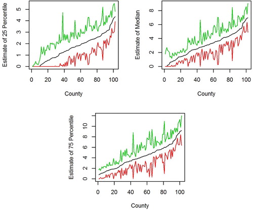
In Figure , county level estimates of the quartiles and the median are plotted along with normal theory 95% prediction intervals. The prediction intervals are calculated for the predictors that ignore the sampling weights. The intervals are defined as , where
is defined in (Equation32
(32)
(32) ), and the lower interval endpoint is truncated at zero. The solid lines correspond to the procedure that ignores the sampling weights. The estimates that account for the sample design, as described in Section 3, are depicted with a dashed line.
Figure 1. Black: predictors of quartiles and the median based on the zero-inflated quantile regression model. Top left: 25 percentile. Top right: median. Bottom: 75 percentile. Solid black line: predictors do not use sampling weights. Dashed black line: predictors incorporate the sampling weights through the preocedure of Section 3.1. Green and red: upper and lower endpoints of 95% prediction intervals.
For this data set, the estimates that account for the informative sample design are nearly indistinguishable from the estimates that ignore the survey weights. Figure shows the estimates for the informative design plotted on the horizontal axis with the corresponding estimates that ignore the sampling weights plotted on the vertical axis. The two sets of estimates nearly lie on the 45 degree line through the origin.
Figure 2. Comparison of predictors that incorporate the modification for informative sampling (x-axis) to predictors that do not use the sampling weights (y-axis). Top left: 25 percentiles. Top right: median. Bottom: 75 percentile.
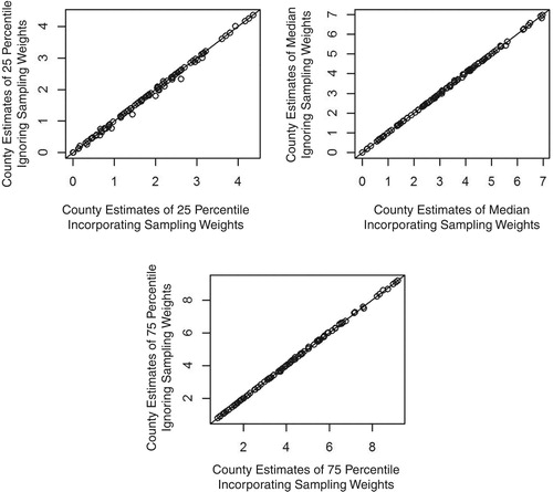
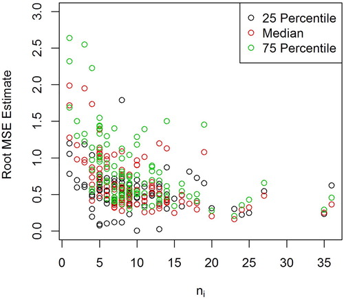
Figure contains square roots of the estimated MSEs plotted against the sample sizes for the areas. The variation in the widths of the intervals is due partly to variation in the sample sizes. The use of the multiplicative lognormal distribution for in (Equation42
(42)
(42) ) also contributes to the variation in the estimated root MSEs. The estimated MSEs from a model with an additive normal random effect show less variation than the estimated MSEs in Figure . Because the additive normal model does not preserve the parameter space for the zero-inflated data, we prefer the multiplicative model (Equation42
(42)
(42) ).
Figure 3. Estimated root mean squared errors plotted against county sample sizes. Estimated mean squared errors are defined in (Equation32(32)
(32) ).
We also compare the estimates with estimated η to the estimates with . The absolute differences between the predictions obtained from the model with estimated η and the predictions from the model with
are less than the estimated standard errors of the predictors with
for all but one area. We present results for estimated η because the
statistic defined in (Equation43
(43)
(43) ) indicates that
. For this data set, estimating η is of little practical significance.
5. Summary and future work
We develop two extensions to the mixed effects quantile regression small area procedure outlined in Section 1.2. One extension accommodates zero-inflated data. The second extension accounts for an informative sample design. To illustrate the procedures, we obtain predictors of quantiles of percolation for Kansas counties, using data from CEAP.
For this data analysis, incorporating the survey weights has only a minor effect on the estimates and estimated root mean squared errors. For this reason, we prefer the simpler predictors that do not use the sampling weights. In other applications, the effects of the sampling weights on the predictors may be important. For such situations, a mean squared error estimator that accounts for the modification for informative sampling would be desirable. Extending the bootstrap procedure of Pfeffermann and Sverchkov (Citation2007) to estimation of quantiles is an area for future work.
For several counties, the estimated root mean squared errors are undesirably large. Expanding the model to incorporate additional covariates or spatial dependence is a possible future direction. A different approach for modelling the zero-inflated data would be to use a censored quantile regression model, as discussed in Section 1.
Supplemental Material
Download PDF (201.1 KB)Disclosure statement
No potential conflict of interest was reported by the authors.
Additional information
Funding
Notes on contributors
Emily Berg
Emily Berg is an assistant professor in statistics, Iowa State University.
Danhyang Lee
Danhyang Lee is an assistant professor in statistics, University of Alabama.
References
- Battese, G., Harter, R., & Fuller, W. (1988). An error-components model for prediction of county crop areas using survey and satellite data. Journal of the American Statistical Association, 83(401), 28–36. doi: 10.1080/01621459.1988.10478561
- Berg, E., & Chandra, H. (2014). Small area prediction for a unit-level lognormal model. Computational Statistics & Data Analysis, 78, 159–175. doi: 10.1016/j.csda.2014.03.007
- Berg, E., & Lee, D. (2019a). Prediction of small area quantiles for the conservation effects assessment project using a mixed effects quantile regression model. Annals of Applied Statistics, Accepted.
- Berg, E., & Lee, D (2019b). Supplement to “Small Area Prediction of Quantiles for Zero-Inflated Data and an Informative Sample Design.” Supplementary material.
- Breslow, N. E., & Clayton, D. G. (1993). Approximate inference in generalized linear mixed models. Journal of the American Statistical Association, 88(421), 9–25.
- Buchinsky, M., & Hahn, J. (1998). An alternative estimator for the censored quantile regression model. Econometrica, 66, 653–671. doi: 10.2307/2998578
- Chambers, R., & Tzavidis, N. (2006). M-quantile models for small area estimation. Biometrika, 93(2), 255–268. doi: 10.1093/biomet/93.2.255
- Chandra, H., & Sud, U. C. (2012). Small area estimation for zero-inflated data. Communications in Statistics-Simulation and Computation, 41(5), 632–643. doi: 10.1080/03610918.2011.598991
- Chernozhukov, V., Fernandez-Val, I., & Galichon, A. (2009). Improving point and interval estimators of monotone functions by rearrangement. Biometrika, 96, 559–575. doi: 10.1093/biomet/asp030
- Dreassi, E., Petrucci, A., & Rocco, E. (2014). Small area estimation for semicontinuous skewed spatial data: An application to the grape wine production in tuscany. Biometrical Journal, 56(1), 141–156. doi: 10.1002/bimj.201200271
- Hall, P., & Maiti, T. (2006). Nonparametric estimation of mean-squared prediction error in nested-error regression models. The Annals of Statistics, 34, 1733–1750. doi: 10.1214/009053606000000579
- Jang, W., & Wang, J. (2015). A semiparameteric Bayesian approach for joint-quantile regression with clustered data. Computational Statistics and Data Analysis, 84, 99–115. doi: 10.1016/j.csda.2014.11.008
- Kim, J. K., & Yu, C. L. (2011). A semiparametric estimation of mean functionals with nonignorable missing data. Journal of the American Statistical Association, 106(493), 157–165. doi: 10.1198/jasa.2011.tm10104
- Koenker, R. (2005). Quantile regression. New York: Cambridge University Press. doi: 10.1017/CBO9780511754098
- Koenker, R., & Ng, P. (2005). Inequality constrained quantile regression. Sankhya: The Indian Journal of Statistics, 67, 418–440.
- Lahiri, S. N., Maiti, T., Katzoff, M., & Parsons, V. (2007). Resampling-based empirical prediction: An application to small area estimation. Biometrika, 94, 469–485. doi: 10.1093/biomet/asm035
- Lyu, X (2018). Empirical Bayes small area prediction of sheet and rill erosion under a zero-inflated lognormal model (Master's Thesis). Iowa State University.
- Opsomer, J. D., Claeskens, G., Ranalli, M. G., Kauermann, G., & Breidt, F. J. (2008). Non-parametric small area estimation using penalized spline regression. Journal of the Royal Statistical Society: Series B (Statistical Methodology), 70(1), 265–286. doi: 10.1111/j.1467-9868.2007.00635.x
- Pfeffermann, D., & Sverchkov, M. (2007). Small-area estimation under informative probability sampling of areas and within the selected areas. Journal of the American Statistical Association, 102(480), 1427–1439. doi: 10.1198/016214507000001094
- Pfeffermann, D., Terryn, B., & Moura, F. A. (2008). Small area estimation under a two-part random effects model with application to estimation of literacy in developing countries. Survey Methodology, 34(2), 235–249.
- Powell, J. L. (1986). Censored regression quantiles. Journal of Econometrics, 32(1), 143–155. doi: 10.1016/0304-4076(86)90016-3
- Rao, J. N., & Molina, I. (2015). Small area estimation. Hoboken, NJ: John Wiley & Sons.
- Searle, S. R., Casella, G., & McCulloch, C. E. (1992). Variance components. New York: John Wiley & Sons.
- Sinha, S. K., & Rao, J. N. K. (2009). Robust small area estimation. Canadian Journal of Statistics, 37(3), 381–399. doi: 10.1002/cjs.10029
- Smith, A. F., & Gelfand, A. E. (1992). Bayesian statistics without tears: A sampling-resampling perspective. The American Statistician, 46(2), 84–88.
- Verret, F., Rao, J. N. K., & Hidiroglou, M. A. (2015). Model-based small area estimation under informative sampling. Survey Methodology, 41(2), 333–347.
- Wang, J., Fuller, W. A., & Qu, Y. (2008). Small area estimation under a restriction. Survey Methodology, 34, 29–36.
- Wischmeier, W. H., & Smith, D. D (1978). Predicting rainfall erosion losses a guide to conservation planning. U.S. Department of Agriculture, Agriculture Handbook No. 537.
- You, Y., & Rao, J. N. K. (2002). A pseudo empirical best linear unbiased prediction approach to small area estimation using survey weights. Canadian Journal of Statistics, 30(3), 431–439. doi: 10.2307/3316146
Appendices
Appendix 1: Initial Estimators
We define an initial estimator of by
(A1)
(A1) where
. Let
be estimates of the variance of the asymptotic distribution of
, estimated with the option se = "ker" in the R function summary.rq. To define an initial estimator of
, define the area-level Fay-Herriot model,
(A2)
(A2) where
has a distribution with mean 0 and variance
, and
has a distribution with mean 0 and variance
for
. The initial estimate of
, denoted by
, is obtained by applying the estimation procedure of Wang, Fuller, and Qu (Citation2008) to the area level model (EquationA2
(A2)
(A2) ). The preliminary estimate of
for
is defined by
(A3)
(A3) We rearrange
for every
to obtain a nondecreasing quantile function (Chernozhukov et al., Citation2009). The estimate
is the kth order statistic of
. Given the initial estimates of the quantile function, we use the procedure in Step 3 of Section 2.2 to obtain estimates
and
for
.
Appendix 2: Details on Estimation of the Power η for the CEAP Data Analysis
Define an initial estimator of as in Appendix 2. Define an initial estimator of η as
where
For
, repeat the following:
Define the updated estimator of
We use the method of Koenker and Ng (Citation2005) to update the estimator of
We modify the method of Jang and Wang (Citation2015) to estimate
and
Define an updated estimator of η as