Multi-outcome longitudinal small area estimation – a case study

ABSTRACT

A recent paper [Thibaudeau, Slud, and Gottschalck (2017). Modeling log-linear conditional probabilities for estimation in surveys. The Annals of Applied Statistics, 11, 680–697] proposed a ‘hybrid’ method of survey estimation combining coarsely cross-classified design-based survey-weighted totals in a population with loglinear or generalised-linear model-based conditional probabilities for cells in a finer cross-classification. The models were compared in weighted and unweighted forms on data from the US Survey of Income and Program Participation (SIPP), a large national longitudinal survey. The hybrid method was elaborated in a book-chapter [Thibaudeau, Slud, & Cheng (2019). Small-area estimation of cross-classified gross flows using longitudinal survey data. In P. Lynn (Ed.), Methodology of longitudinal surveys II. Wiley] about estimating gross flows in (two-period) longitudinal surveys, by considering fixed versus mixed effect versions of the conditional-probability models and allowing for 3 or more outcomes in the later-period categories used to define gross flows within generalised logistic regression models. The methodology provided for point and interval small-area estimation, specifically area-level two-period labour-status gross-flow estimation, illustrated on a US Current Population Survey (CPS) dataset of survey respondents in two successive months in 16 states. In the current paper, that data analysis is expanded in two ways: (i) by analysing the CPS dataset in greater detail, incorporating multiple random effects (slopes as well as intercepts), using predictive as well as likelihood metrics for model quality, and (ii) by showing how Bayesian computation (MCMC) provides insights concerning fixed- versus mixed-effect model predictions. The findings from fixed-effect analyses with state effects, from corresponding models with state random effects, and fom Bayes analysis of posteriors for the fixed state-effects with other model coefficients fixed, all confirm each other and support a model with normal random state effects, independent across states.

KEYWORDS:

• Bayesian computation
• Current Population Survey
• generalised logistic regression
• gross flows
• mixed-effects model
• small-area estimation

1. Introduction

The general problem considered here is modelling and estimation for multi-period longitudinal survey data $({\mathbf{X}}_i,Y_i)$, where i indexes the first-period responders with complete multi-period data, ${\mathbf{X}}_i$ is a covariate vector including early-period survey outcomes, and $Y_i$ is a later-period survey outcome. Because the unit indices i refer to responders who are also matched (for example, at the household level) to later-period responders, they will have weights $w_i$ incorporating inverse single-inclusion probablities for the survey as well as adjustments for nonresponse both at early and later stages. Although such adjustments (by cell-based ratio adjustment or calibration or raking) yield weights that are themselves not interpretable as inverse inclusion probabilities, we will ignore this distinction throughout the present paper as is customary in the survey literature.

The approach taken in this paper continues one developed in papers of Pfeffermann, Skinner, and Humphreys (1998), Thibaudeau, Slud, and Gottschalck (2017), and a book-chapter Thibaudeau, Slud, and Cheng (2019). The main idea is a ‘hybrid’ analysis combining model-free survey-weighted Horvitz-Thompson (HT) estimation (Särndal, Swensson, & Wretman, 1992) for ${\mathbf{X}}_i$ variables with conditionally specified parametric models for outcomes $Y_i$ given ${\mathbf{X}}_i$. The combined approach allows counts in small cells cross-classifying $({\mathbf{X}}_i,Y_i)$, including ‘gross flows’ in a longitudinal context (such as that of Fienberg, 1980), to be estimated more accurately than design-based methodology would allow while restricting parametric models purely to conditional specifications. So we treat antecedent categorical variables ${\mathbf{X}}_i$ through HT survey estimation, when the cross-classified cells defined by ${\mathbf{X}}_i$ configurations are large enough so that HT estimates of the cell totals and proportions are sufficiently accurate. The parametric models considered here are generalised logistic or loglinear models (Agresti, 2013, Ch. 9) for outcomes $Y_i$ in terms of covariates ${\mathbf{X}}_i$. If $Y_i$ takes the categorical values $y=1,2,\dots ,H$, then we treat the final category H as a reference and express conditional probabilities given ${\mathbf{X}}_i=\mathbf{x}$ in terms of parameter $\mathit{\theta }=({\text{β}}^{\left(z\right)},z=1,\dots ,H-1)$ for $y=1,\dots ,H-1$ as: (1) $\begin{array}{r}P(Y_i=y|{\mathbf{X}}_i=\mathbf{x})=\exp \left({\mathbf{x}}^{\prime }{\text{β}}^{\left(y\right)}\right)/\left(1+\sum _{z=1}^{H-1}\exp \left({\mathbf{x}}^{\prime }{\text{β}}^{\left(z\right)}\right)\right)\end{array}$(1) (2) $\begin{array}{rl}P(Y_i& =H|{\mathbf{X}}_i=\mathbf{x})=1/\left(1+\sum _{z=1}^{H-1}\exp \left({\mathbf{x}}^{\prime }{\text{β}}^{\left(z\right)}\right)\right)\end{array}$(2) Here the covariates ${\mathbf{X}}_i$ and values $\mathbf{x}$ and parameter-vectors ${\text{β}}^{\left(z\right)}=({\text{β}}_1^{\left(z\right)},\dots ,{\text{β}}_p^{\left(z\right)})$ all have the same dimension p, so that the unknown parameter $\mathit{\theta }$ in the fixed-effect model has dimension $p\cdot (H-1)$. Within the same model, we consider also the case of random area-level intercepts for a categorical component of ${\mathbf{X}}_i$ with r<p levels. In the mixed-effect case, let the first r components of each of the vectors ${\text{β}}^{\left(z\right)}$ denote the random intercepts, that is, the coefficients ${\text{β}}_j^{\left(z\right)}$ of the dummy indicators ${\mathbf{X}}_{i,j}$ (for ith survey unit) of belonging to area j. In this mixed model, the random-intercepts ${\alpha }_{j,z}={\text{β}}_j^{\left(z\right)}$ are random and unobserved for $j=1,\dots ,r$ and $z=1,\dots ,H-1$ and the unknown statistical parameters are $({\text{β}}_k^{\left(z\right)},k=r+1,\dots ,p,z=1,\dots ,H-1)$ together with the unknown variance components governing the (usually multivariate-normal mean-0) random intercepts ${\alpha }_{j,z}$. Generally, the random effects ${\alpha }_{j,z}$ are assumed uncorrelated across distinct z, and in the simplest random-effects model, also uncorrelated across $j=1,\dots ,r$, with variances ${\sigma }_z^2$ depending only upon z.

The particular dataset that we consider throughout the paper, following Thibaudeau et al. (2019), is from June and July 2017 monthly data for selected U.S. states in the US Current Population Survey (CPS). The CPS is a rotating household panel survey collecting information on many aspects of the labour force. We focus on estimating uncommon changes in the standard 3-category labour force status – employed (Emp), unemployed (Unemp) or not in labour force (NILF) – between the two months, and on the classification of the gross flows generated by those changes. Because the single-period cross-classified June 2017 totals are estimated in design-based fashion, our models express conditional status changes given cross-classified first-period status. In our data, variables $Y_i$ are the person-level July 2017 labour-force status (STAT07) and ${\mathbf{X}}_i$ include June 2017 labour-force status (STAT06), 4-category age-group (AGE06 = 65+, 55-64, 35-54, 0-34), indicator of college education (EDUC06), and state of residence (ST, one of 16 small or medium-sized states from New England, the South and the Southwest). By the CPS design, 75% of surveyed addresses in one panel month are included also in the following month. However, there is a nontrivial issue of matching persons across time-periods: it is the addresses that are followed up over successive months in CPS although different individuals may be living there. In our CPS data application, matching was done by filtering the monthly person-level CPS files for the two consecutive months, June and July 2017. We checked first that the person's household identifier was scheduled under the rotational pattern to be sampled in both months, second that (post-editing) the main employment category field was not blank for the sampled person record in either month, and third, that the person-level demographic (race and ethnicity) variables were not missing and were identical for both months, and that the age in the second month was either equal to or one larger than the age in the first month. The dataset contains records for roughly 18,000 persons which, after aggregation into cells determined by covariate ${\mathbf{X}}_i$, correspond to 384 cross-classified STAT06 by EDUC06 by AGE06 by ST cells, of which 349 are nonempty with sizes ranging from 1 to 262 (with median 29 and mean 52.2).

2. Data analysis

The goal of this data analysis is to find parsimonious predictive models passing tests of statistical adequacy and predictive accuracy. Adequacy and the comparison between fixed- and mixed-effect models will be assessed primarily through likelihoods, while predictive accuracy will be examined using tools related to Receiver Operating Characteristic (ROC) curves.

2.1. Preliminary findings

Thibaudeau et al. (2019) analysed and compared various models for the CPS 16-state data, reporting detailed results for four models: one fixed-effect generalised logistic model (1(1) $\begin{array}{r}P(Y_i=y|{\mathbf{X}}_i=\mathbf{x})=\exp \left({\mathbf{x}}^{\prime }{\text{β}}^{\left(y\right)}\right)/\left(1+\sum _{z=1}^{H-1}\exp \left({\mathbf{x}}^{\prime }{\text{β}}^{\left(z\right)}\right)\right)\end{array}$(1) )–(2(2) $\begin{array}{rl}P(Y_i& =H|{\mathbf{X}}_i=\mathbf{x})=1/\left(1+\sum _{z=1}^{H-1}\exp \left({\mathbf{x}}^{\prime }{\text{β}}^{\left(z\right)}\right)\right)\end{array}$(2) ) in terms of ST, AGE06, EDUC06, STAT06 and one with the additional interaction term STAT06:AGE06, and mixed-effect models in which the 16 fixed-effect coefficients ST are replaced by a single overall Intercept along with unstructured-variance mean-0 random intercepts for the 16 states. That chapter stated that interaction-terms other than STAT06:AGE06 were found to be predictively ineffective, and found the larger fixed-effect and mixed-effect models to be statistically adequate (in terms of deviance) with $G^2$ respectively equal to 678.1 and 737.5 on 712 and 742 residual degrees of freedom; the smaller fixed-effect model (without pairwise interaction) to be only barely inadequate ($G^2=792.9$ on 724 df), and the smaller mixed model clearly inadequate (with $G^2=854.3$ on 754 df).

For simplicity, and to facilitate rapid fitting and comparison of mixed logistic models within R, we performed further model exploration by exploiting the observation that model (1(1) $\begin{array}{r}P(Y_i=y|{\mathbf{X}}_i=\mathbf{x})=\exp \left({\mathbf{x}}^{\prime }{\text{β}}^{\left(y\right)}\right)/\left(1+\sum _{z=1}^{H-1}\exp \left({\mathbf{x}}^{\prime }{\text{β}}^{\left(z\right)}\right)\right)\end{array}$(1) )–(2(2) $\begin{array}{rl}P(Y_i& =H|{\mathbf{X}}_i=\mathbf{x})=1/\left(1+\sum _{z=1}^{H-1}\exp \left({\mathbf{x}}^{\prime }{\text{β}}^{\left(z\right)}\right)\right)\end{array}$(2) ) implies standard logistic regression models for the same coefficient vectors ${\text{β}}^{\left(z\right)}$ when restricted to data records for which $Y_i$ is equal either to z or H, for each $z=1,\dots ,H-1$. On the the CPS data, where H = 3, an added motivation for separate logistic-regression analyses is that the person-level decisions reflected in outcomes Emp07 vs. NILF07 (on records for which $Y_i$ is not Unemp07) might be quite different from those in outcome Unemp07 vs. NILF07. Thibaudeau et al. (2019) found within the fixed-effect models, the point estimates from two separate logistic regressions showed only very smalll differences from the MLEs for the combined model (1(1) $\begin{array}{r}P(Y_i=y|{\mathbf{X}}_i=\mathbf{x})=\exp \left({\mathbf{x}}^{\prime }{\text{β}}^{\left(y\right)}\right)/\left(1+\sum _{z=1}^{H-1}\exp \left({\mathbf{x}}^{\prime }{\text{β}}^{\left(z\right)}\right)\right)\end{array}$(1) )–(2(2) $\begin{array}{rl}P(Y_i& =H|{\mathbf{X}}_i=\mathbf{x})=1/\left(1+\sum _{z=1}^{H-1}\exp \left({\mathbf{x}}^{\prime }{\text{β}}^{\left(z\right)}\right)\right)\end{array}$(2) ). Indeed, the interquartile ranges of absolute differences of the two sets of parameter estimates were $(0.015,0.039)$ for the no-interaction Emp07 model, $(0.018,0.048)$ for the no-interaction Unemp07 model, and respectively $(0.007,0.044)$ and $(0.004,0.041)$ for the respectively corresponding models with STAT06:AGE06 interactions. Moreover, the loss of efficiency was very small in passing from the separate logistic to a combined generalised-logistic model. The ratio of estimated standard errors of the combined-model coefficients to those of the separate-model coefficients ranged from 0.949 to $0.988$ for the Emp07 no-interaction model, from 0.908 to 0.99 (with only 3 below 0.940) for the Unemp07 no-interaction model, from 0.956 to 0.997 for the Emp07 model with interaction, and from 0.915 to 0.997 for the Unemp07 model with interaction terms.

We next address variable-selection, separately for Emp07 vs. NILF07 and Unemp07 vs. NILF07 logistic regression models respectively based on approximately 17,500 and 8000 (rounded numbers of) person-records. Throughout, we consider 3 labelled fixed-effect models: (3) $\begin{array}{r}\mathbf{F}\mathbf{0}\mathbf{:}\mathrm{S}\mathrm{T}\mathrm{A}\mathrm{T}06+\mathrm{A}\mathrm{G}\mathrm{E}06+\mathrm{E}\mathrm{D}\mathrm{U}\mathrm{C}06,\mathbf{F}\mathbf{1}\mathbf{:}\mathbf{F}\mathbf{0}+\mathrm{S}\mathrm{T},\mathbf{F}\mathbf{2}\mathbf{:}\mathbf{F}\mathbf{1}+\mathrm{S}\mathrm{T}\mathrm{A}\mathrm{T}06:\mathrm{A}\mathrm{G}\mathrm{E}06\end{array}$(3) Model F0 has an Intercept, and therefore 7 coefficients in each of the Emp07 and Unemp07 models; F1 adds 15 predictor columns (although it is convenient to delete the overall Intercept and let each state contribute its own); and finally, model F2 has design matrix $\mathbf{X}$ including interaction term STAT06:AGE06 with a total of 28 columns. The first-month labour-status STAT06 is clearly the strongest predictor in both models, with the main effects AGE06 also obviously important. However, beyond these predictors the value of EDUC06 and ST dummy-variables is much less clear, in the side-by-side Analysis of Deviance tables of Table 1 for those corresponding models. First, in the Emp07 model both EDUC06 and ST are important predictors, as is the interaction STAT06:AGE06, but further (pairwise) interactions are not, and the model with all of these fixed-effect predictive terms still falls short of statistical adequacy, in the sense that the residual deviance of 381 referred to a chi-square on 300 degrees of freedom still has p-value 0.001. On the other hand, in the Unemp07 model, EDUC06 is not a useful predictor, and the ST dummy indicators overall not very useful, while the STAT06:AGE06 interaction terms do make a difference to model predictions. The model omitting EDUC06 and ST has residual deviance 347 on 322 df, achieving p-value 0.16 indicating model adequacy.

Table 1. Analysis of Deviance tables for separate logistic regressions of Emp07 and of Unemp07 (each vs. NILF07) based on CPS June-July 2017 dataset. (Deviances rounded to 4 significant figures.)

	Emp07 vs NILF07				Unemp07 vs NILF07
	df	Dev	Res.df	Res.Dev	df	Dev	Res.df	Res.Dev
NULL			327	18860			333	1912
STAT06	2	18140	325	717.3	2	1391	331	521.2
AGE06	3	209.5	322	507.8	3	137.2	328	384.1
EDUC06	1	16.6	321	491.1	1	1.8	327	382.3
ST	15	34.6	306	456.5	15	18.5	312	363.7
STAT06:AGE06	6	75.4	300	381.2	6	35.0	306	328.7
STAT06:ST	30	31.0	270	350.1	30	39.1	276	289.7

The Emp07 model is based on many more person-records than Unemp07, but Emp07 is much better predicted by first-month employed status Emp06 (correlation 0.91) than Unemp07 is by Unemp06 (correlation 0.53). There are interestingly different State intercepts for Emp07, but not so much for Unemp07. In the combined (generalised-logistic, fixed-effect) model including all F2 terms, for both outcomes Emp07, Unemp07 there are similar numbers of states showing significant contrasts ${\text{β}}_j^{\left(z\right)}-{\text{β}}_1^{\left(z\right)}$ (all positive) from AL=1, especially for j corresponding to LA, ME, VT when z = 1 (Emp07) and for j correspnding to LA, NH with z = 2 (Unemp07), although the contrasts for the Emp07 model are larger measured in standard-deviation units than for Unemp07.

Thus both of the separate logistic regression models indicate similar but not the same predictor variables. The model for Emp07 is not quite statistically adequate as indicated by residual deviance, while that for Unemp07 does seem adequate based on fewer predictors. We re-examine these conclusions about the predictive models below from the viewpoint of state random effects and of predictive accuracy.

2.2. Software for statistical analysis

This subsection concerns the functionality of SAS and R (R Core Team, 2017) for estimating generalised logistic regression models with mixed effects. The main issue is which types of models (two- or multiple-outcome) are allowed and whether loglikelihoods involving random effects are computed to high accuracy or approximated. In all the packages that compute maximum likelihood (ML) estimates using accurately evaluated mixed-effect loglikelihoods, the numerics are based ultimately on adaptive Gaussian quadrature as introduced by Pinheiro and Bates (1995), although at least one (GLMMadaptive in R) also uses EM.

1. SAS PROC NLINMIX can handle everything at the cost of customised programming, with GLIMMIX handling mixed logistic and generalised logistic regressions (Stroup, 2013) using accurate likelihood approximation.

2. The estimation of generalised logistic (multiple-outcome) fixed-effect regression models in R can be done via Poisson regression in glm or within the nnet or mlogit packages, but no method in R exists for accurate (or convenient) computation of mixed-effect likelihoods and MLEs in these models.

3. If the model is split into two separate ordinary logistic regressions with random-effect terms ${ϵ}_{i,j}$ independent across outcomes j = 1, 2, then a few different R packages can handle different mixed-effect models: (a) glmmML accurately and rapidly computes maximum-likelihood estimates of regression coefficients θ together with random-effect variance for a random-intercept model; (b) the function glmer in package lme4 accurately fits mixed-effect GLMs in settings with single-level (possibly multivariate) random-effects, or fits approximately (via Laplace approximation) for multilevel random-effects; (c) GLMMadaptive computes MLEs in GLMs with single-level (multivariate) random effects. The packages agree closely on point estimates in the case of single random intercepts, but even there may disagree on estimated standard deviation of random effect, and this discrepancy in estimating variance structure is even greater in the case of multiple random effects (at the same cluster level).

4. There are other approximations (via penalised quasilikelihood and MCMC) for mixed-model MLEs in other R packages, which we do not address further here.

5. For Bayesian MCMC analyses of GLMs, R packages like BRugs and rjags provide a front-end to the BUGS and JAGS Bayesian MCMC packages, but in our attempts to use them on the data example of this paper, they were very slow. An alternative idea, custom-coded in R, seems to work much better in the present large-sample setting. See Subsection 2.5 for details.

2.3. Assessments of fixed-effect model quality

We have already seen, in Section 2.1, a preliminary assessment of model fit through loglikelihoods and analysis of deviance. But those are not the only metrics of model quality. The separate fixed-effect logistic models can be viewed as generating a rule for predicting whether a person is Employed or NILF (among those not unemployed) [and respectively Unemployed or NILF, among those not employed] in the second month given the covariate for the first month. The prediction rule takes the form (4) $\begin{array}{rl}{\widehat{\mathrm{E}\mathrm{m}\mathrm{p}}}_i& =1\mathrm{i}\mathrm{f}{\mathrm{U}\mathrm{n}\mathrm{e}\mathrm{m}\mathrm{p}}_{\mathrm{i}}=0\mathrm{a}\mathrm{n}\mathrm{d}{\mathbf{X}}_{\mathrm{i}}^{\mathrm{\prime }}{\widehat{\text{β}}}^{\left(1\right)}\ge {\mathrm{c}}_1\end{array}$(4) (5) $\begin{array}{rl}{\widehat{\mathrm{U}\mathrm{n}\mathrm{e}\mathrm{m}\mathrm{p}}}_i& =1\mathrm{i}\mathrm{f}{\mathrm{E}\mathrm{m}\mathrm{p}}_{\mathrm{i}}=0\mathrm{a}\mathrm{n}\mathrm{d}{\mathbf{X}}_{\mathrm{i}}^{\mathrm{\prime }}{\widehat{\text{β}}}^{\left(2\right)}\ge {\mathrm{c}}_2\end{array}$(5) where $c_1,c_2$ are some thresholds to be chosen according to the relative importance of false predictions of Employed or Unemployed versus NILF. With specific choices of $c_1=0.4055$ and $c_2=-0.4055$ equal to logistic quantiles 0.6 and 0.4, the predictive success of (4(4) $\begin{array}{rl}{\widehat{\mathrm{E}\mathrm{m}\mathrm{p}}}_i& =1\mathrm{i}\mathrm{f}{\mathrm{U}\mathrm{n}\mathrm{e}\mathrm{m}\mathrm{p}}_{\mathrm{i}}=0\mathrm{a}\mathrm{n}\mathrm{d}{\mathbf{X}}_{\mathrm{i}}^{\mathrm{\prime }}{\widehat{\text{β}}}^{\left(1\right)}\ge {\mathrm{c}}_1\end{array}$(4) ) and (5(5) $\begin{array}{rl}{\widehat{\mathrm{U}\mathrm{n}\mathrm{e}\mathrm{m}\mathrm{p}}}_i& =1\mathrm{i}\mathrm{f}{\mathrm{E}\mathrm{m}\mathrm{p}}_{\mathrm{i}}=0\mathrm{a}\mathrm{n}\mathrm{d}{\mathbf{X}}_{\mathrm{i}}^{\mathrm{\prime }}{\widehat{\text{β}}}^{\left(2\right)}\ge {\mathrm{c}}_2\end{array}$(5) ) can be seen from $2\times 2$ cross-tabulations in Table 2. The tables show remarkably little difference between the least and most detailed models for each of the Emp07 vs. NILF07 and Unemp06 vs. NILF07 logistic regressions. In each setting, the correctness of the model-based predictions mostly reflects that the employment status in July 2017 (the second month) is the same as in June 2017. (This is true for 95% of those Employed in June, 50% of those Unemployed, and 94% of NILF persons. In both the upper and lower halves of Table 2, the $2\times 2$ cross-tabulation for the intermediate model with ST intercepts but no interactions agrees precisely (before rounding) with the tabulation for the most detailed model.

Table 2. Rounded Cross-tabulations of counts vs. predictions of Emp07 and Unemp07 (each vs. NILF07) from two fixed-effect logistic regression models under model F0 with only the main effects STAT06, AGE06, EDUC06.

	Emp07	NILF07
Emp.Pred	10000	350
NILF.Prd	400	7000
	Unemp07	NILF07
Unemp.Prd	250	150
NILF.Pred	250	7200

Notes: The corresponding cross-tabulated entries when predictions are made with model F2, which is based on the terms of F0 augmented by terms for ST, STAT06:AGE06, are different from those shown in the Emp07 vs. NILF07 table by at most 4 in all cells and in the Unemp07 vs. NILF07 by at most 26 in all cells.

With the thresholds $c_1,c_2$ unspecified, the predictive quality of the separate models can be summarised in terms of the so-called ROC curves, defined for the Emp07 model as the trace over all real $c_1$ of the points $\begin{array}{rl}& \left(\frac{\sum _i(1-{\mathrm{U}\mathrm{n}\mathrm{e}\mathrm{m}\mathrm{p}07}_{\mathrm{i}}){\mathrm{E}\mathrm{m}\mathrm{p}07}_{\mathrm{i}}\mathrm{I}[{\mathbf{X}}_{\mathrm{i}}^{\prime }{\widehat{\text{β}}}^{\left(1\right)}\ge {\mathrm{c}}_1]}{\sum _i(1-{\mathrm{U}\mathrm{n}\mathrm{e}\mathrm{m}\mathrm{p}07}_{\mathrm{i}}){\mathrm{E}\mathrm{m}\mathrm{p}07}_{\mathrm{i}}},\right.\\ & \left.\frac{\sum _i(1-{\mathrm{U}\mathrm{n}\mathrm{e}\mathrm{m}\mathrm{p}07}_{\mathrm{i}}){\mathrm{N}\mathrm{I}\mathrm{L}\mathrm{F}07}_{\mathrm{i}}\mathrm{I}[{\mathbf{X}}_{\mathrm{i}}^{\prime }{\widehat{\text{β}}}^{\left(1\right)}\ge {\mathrm{c}}_1]}{\sum _i(1-{\mathrm{U}\mathrm{n}\mathrm{e}\mathrm{m}\mathrm{p}07}_{\mathrm{i}}){\mathrm{N}\mathrm{I}\mathrm{L}\mathrm{F}07}_{\mathrm{i}}}\right)\end{array}$ with ROC in the Unemp07 model similarly defined as the trace of pairs of relative frequencies of correct predictions of ${\mathrm{U}\mathrm{n}\mathrm{e}\mathrm{m}\mathrm{p}07}_{\mathrm{i}}$ over all choices of threshold $c_2$. These ROC pictures are conveniently overplotted with function colAUC in the caTools package in R for the F0, F1 and F2 models, but look visually identical. The commonly used Area Under Curve (or AUC) statistic for ROC curves is 0.973 for the F0 and 0.974 for the F2 Emp07 models in Table 2, with respective AUCs of 0.912 and 0.917 for the Unemp07 models. In the Unemp07 case, the ROC for F2 shows very small but visible superiority in correct prediction of NILF07 when the predicted probability plogis$\left({\mathbf{X}}_i^{\prime }{\text{β}}^{\left(2\right)}\right)$ falls in the range $(0.1,0.4)$, which is in fact the predominant range where NILF predictions fall for the Unemp07 models under consideration.

Thus the ROCs for the separate logistic regression models slightly disagree with likelihood-based criteria of fit like AIC: the ROCs indicate no meaningful difference between models based on predictors F0, F1 or F2, while the likelihood criteria suggest that F2 is better for discriminating between Unemp07, NILF07 based on previous-month data but not for discriminating between Emp07, NILF07.

Further discussion of predictive effectiveness of models should recognise that there are three outcomes in the current data-setting, while the separate logistic models and their ROCs account for only two outcomes each. The literature does in fact contain extensions of ROCs for multiple-outcome predictions of which the most cited (Hand & Till, 2001), summarises predictions for multiple outcomes by averaging all of the pairwise AUC comparisons. Li and Fine (2008) give a broader mathematical survey of multiple-outcome ROC extensions. We consider a slightly different approach, which differs in the way 3-outcome predictions are parameterised.

In the two-outcome case, a model-based prediction rule can be described either as choosing the first outcome when its predicted probability is above a threshold, or as the optimal probability-based prediction minimising loss with respect to a fixed linear combination of costs of incorrect predictions weighted by outcome-specific costs (and prior probabilities). The analogy for multiple outcomes based on weights $w_j$, proportional to the product of outcome-specific prior probabilities and incorrect-prediction costs and summing to 1, is a prediction-rule in terms of predicted outcome probabilities ${\hat{p}}_j$ which selects outcome k if $w_k{\hat{p}}_k=\underset{j}{max}\left\{w_j{\hat{p}}_j\right\}$ (and the smallest k with this property, in case of ties). With this prediction rule on a fixed 3-outcome dataset, we obtain for each weight probability-vector $\mathbf{w}=(w_1,w_2,w_3)$, the proportion $\pi \left(\mathbf{w}\right)$ of correct predictions. This function of $\mathbf{w}$ defines a surface over the probability simplex of $\mathbf{w}$ values viewed as a triangle in barycentric coordinates. A perspective or contour plot of this surface can be created using the new R package ggtern. The surfaces for different predictive models (e.g., F0 through F2) on a fixed dataset can be compared, but visual comparison of similar perspective or contour plots is unrewarding. Instead, we compare the different models discussed in Tables 1 and 2 on our CPS dataset with respect to the volume under the $\pi \left(\mathbf{w}\right)$ surface, which could be done analytically but is done here by a small Monte-Carlo calculation. The resulting estimate on our data (averaged over the same set of ${10}^5$ randomly selected w's in the 3-simplex for all 3 models) is that the volume under the $\pi \left(\mathbf{w}\right)$ surface is 0.904 for F0 and 0.905 for F2. 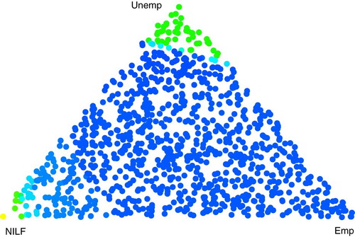Figure 1 shows that for values w that do not heavily emphasise NILF or Unemp, the probability $\pi \left(\mathbf{w}\right)$ of correct model-based selection is higher, uniformly close to 0.93.

Figure 1. False-colour graph of proportions $\pi \left(\mathbf{w}\right)$ of correct prediction among outcomes Emp07, Unemp07, NILF07 at 700 weight-vectors w in barycentric coordinates for CPS data with 3-level outcome STAT07 in generalised logistic model with predictors F0. Colors range from bright yellow at correct-prediction proportion 0.4 to bright blue at 0.95.

2.4. Goodness of fit for mixed-effect models

Likelihood-based variable selection from the analysis of deviance showed in Table 1 that models F1 and F2 are preferred over F0 in the separate Emp07 logistic model but not the Unemp07 model. In the generalised logistic model combining all three outcomes STAT07, the rounded deviances, equal to $-2$ times loglikelihoods, for models F0, F1 and F2 are $-8959,-8897,-8781$, so that the F1 vs. F0 deviance difference is 62 on 30 df and the F2 vs. F1 deviance difference is 116 on 12 df. So even more strongly in the combined generalised logistic regression, the more detailed models are the preferred ones despite the finding in Section 2.5.3 that the metrics for outcome-prediction quality do not improve from F0 to F2.

When the higher-dimensional in a sequence of fixed-effect models are found significantly better in likelihood but not in improved prediction, it is natural to check whether a random-effect version of the detailed models can more parsimoniously attain statistical adequacy. We do this by comparing various mixed-effect models fitted under heading 3. in Section 2.2. Recall that the fixed-effect model F0 included terms only for the main effects (STAT06, AGE06, EDUC06), and model F2 added ST main-effects and STAT06:AGE06 interactions. In this Section, we compare fixed- and mixed-effect versions of F2 for the separate z = 1 (Emp07) and z = 2 (Unemp07) logistic regressions. What we mean by ‘mixed-effect version’ is that the coefficients of the ST terms in F2 are regarded as independent (across state) $\mathcal{N}(0,{\sigma }_z^2)$ random variates, and it is convenient to compare these mixed-effect model log- likelihoods with corresponding log-likelihoods for the fixed-effect model (denoted F2.0 from now on) with terms (STAT06, AGE06, EDUC06, STAT06:AGE06) and an overall intercept but no ST terms.

We begin by examining (2-outcome) logistic regression models with independent (normal) random ST intercepts in the presence of the fixed effect model F2.0, which has 13 parameters for coefficients of terms Int + STAT06 + AGE06 + EDUC06 + STAT06:AGE06), while the random-ST-intercept model has an additional scale parameter ${\sigma }_z$, and the fixed-effect F2 model had 15 additional regression-coefficient parameters beyond F2.0. In fitting the random-intercept regression models, R functions glmer (in package lme4), glmmML (in the package of the same name), and mixed_model (in package GLMMadaptive) can all be used to check one another. In the Emp07 model, the glmmML function finds that the ML-estimated value of the random-intercept standard deviation is $\hat{\sigma }=0.1645$ and the estimated standard deviation for $\hat{\sigma }$ is 0.0598. The other R functions for fitting this random-intercept model make it harder to calculate the standard deviation of $\hat{\sigma }$, although it can be done via glmer with approximately the same result by finding numerical second derivatives of the loglikelihood at the MLE with respect to the parameters ${\text{β}}^{\left(1\right)},\sigma$. So this analysis suggests unsurprisingly that the random-effect standard deviation in the Emp07 model is significantly different from 0. Another formal significance test of adequacy of the F2.0 fixed-effect model versus the alternative with nonzero random ST intercepts is based on the likelihood-ratio (LR) statistic equal to the residual deviance from the fixed-effect model minus the residual deviance from the random-intercept model, given by glmmML as 415.2−410.3 = 4.9. (This same deviance difference is confirmed from the glmer model fit and loglikelihood function.) Because the null hypothesis puts the σ parameter at the boundary of the allowed parameter space $[0,\mathrm{\infty })$, the large-sample reference distribution for this LR statistic is the mixture with weights 1/2 and 1/2 of a point-mass at 0 and a ${\chi }_1^2$ distribution (Self & Liang, 1987, Case 5, p. 608), resulting in a p-value of  $0.5\cdot (1-\mathrm{p}\mathrm{c}\mathrm{h}\mathrm{i}\mathrm{s}\mathrm{q}(4.9,1\left)\right)=0.013$. This analysis confirms that state intercepts matter, in a likelihood sense, although the random-intercept F2.0 model has much smaller residual deviance than the fixed-effect F2 model. Yet, as we saw in Section 2.5.3, the more precise estimation of state intercepts as fixed effects hardly affects prediction. We also confirmed that the predicted probabilities for Emp07 versus NILF07 from the F2.0 model with random state-effects were almost indistinguishable from those produced by the fixed-effect F2 model.

Estimation of the random-intercept standard deviation $\hat{\sigma }$ for the Unemp07 model results in a convincingly non-significant test of F2.0 versus its random-ST-intercept counterpart, with $\hat{\sigma }=0.033$ and its estimated standard deviation equal to 0.285, and this is confirmed by a LR statistic value 0.01 (obtained from glmmML or lme4).

Additional analyses were done to test whether a ST:STAT06 or ST:AGE06 random effect might be significant for Emp07 vs. NILF07 models enlarging the random ST-intercept model. Whether or not the further random-effect terms were specified to be independent of the ST-intercept effects, these models showed (via GLMMadaptive, the only one of these R packages to calculate loglikelihoods accurately rather than with the Laplace or other approximations) only insignificant deviance improvements. Again in this LR analysis, the theory of Self and Liang (1987) concerning variance-component parameters on the 0-boundary of their feasible parameter space is needed to establish the reference distribution for valid LR testing as a mixture of ${\chi }_k^2$ densities with k ranging up to the number of additional parameters considered.

Since a dot-plot of the fixed state-effects in the Emp07 F2 model (not shown) does not suggest a normal distribution, one might seek additional information on the usefulness of random ST-intercept models by varying the random effect distribution. Rather than addressing this question directly for the CPS data in terms of the separate logistic regression models, we consider it in connection with Bayesian analysis of the ST fixed-effect intercepts within the 3-outcome generalised logistic model (1(1) $\begin{array}{r}P(Y_i=y|{\mathbf{X}}_i=\mathbf{x})=\exp \left({\mathbf{x}}^{\prime }{\text{β}}^{\left(y\right)}\right)/\left(1+\sum _{z=1}^{H-1}\exp \left({\mathbf{x}}^{\prime }{\text{β}}^{\left(z\right)}\right)\right)\end{array}$(1) )–(2(2) $\begin{array}{rl}P(Y_i& =H|{\mathbf{X}}_i=\mathbf{x})=1/\left(1+\sum _{z=1}^{H-1}\exp \left({\mathbf{x}}^{\prime }{\text{β}}^{\left(z\right)}\right)\right)\end{array}$(2) ).

2.5. Bayesian analysis

The foregoing analyses have all been frequentist, with random state effects modelled parametrically within the mixed-effects models studied. Another approach would be to view fixed state-effects as unknown parameters within a Bayesian framework. A Bayesian analysis in the present context can provide insight into the sampling distributions of the state fixed-effect parameter estimates, both conditionally given the other fixed-effect parameter estimates and unconditionally, and on the meaning and approppriateness of a random-effects analysis. The Bayesian computational steps turn out to be easy in this data example and allow a relatively simple way of checking that state-effect contrasts are not an artifact. Other benefits of the Bayesian analysis are discussed by Gelman and Hill (2007), but we emphasise those with direct frequentist interpretations.

A well-known theorem of Bayesian theory is the Bernstein-von Mises Theorem (Bickel & Doksum, 2015, Section 6.2.3), sometimes called by Bayesian authors the ‘Bayesian Central Limit Theorem’. It says that under regularity conditions similar to those guaranteeing asymptotic normality of MLE's, and under prior distributions smooth and with broad support with respect to the unknown statistical parameter, in large data samples the posterior distribution of the parameter θ is approximately multivariate normal centred at the MLE $\hat{\theta }$ and with variance-covariance equal to $\left(\hat{\mathcal{I}}\right(\hat{\theta }){)}^{-1}$, the inverse of the observed (empirical) Fisher information matrix. The relevance of this theorem in the large-sample CPS dataset is twofold: (i) it is the benchmark against which computed posterior densities can be compared, and (ii) it provides an excellent ‘proposal distribution’ for the Metropolis-Hastings Algorithm underlying Markov-Chain Monte-Carlo computation of the posterior density.

In the CPS dataset, it turned out that the estimated standard deviation of the state effect in the Emp07 vs. NILF07 random-intercept logistic regression model was 0.164, while the estimated standard errors of the state intercepts in the fixed-effects F2 model ranged from 0.15 to 0.22. Similarly, the estimated standard errors of the state intercepts in the fixed-effects F2 logistic regression model for Unemp07 vs. NILF07 ranged from 0.22 to 0.38. In addition, the 3-outcome generalised logistic F2 regression estimates of state fixed-effects standard errors (16 for each of the sets of coefficients ${\widehat{\text{β}}}^{\left(z\right)}$ for z = 1, 2 in Equation (1(1) $\begin{array}{r}P(Y_i=y|{\mathbf{X}}_i=\mathbf{x})=\exp \left({\mathbf{x}}^{\prime }{\text{β}}^{\left(y\right)}\right)/\left(1+\sum _{z=1}^{H-1}\exp \left({\mathbf{x}}^{\prime }{\text{β}}^{\left(z\right)}\right)\right)\end{array}$(1) )) agreed reasonably closely with the estimates from the separate logistic regressions. However, the correlations between the intercepts for the same state in ${\text{β}}^{\left(1\right)}$ and ${\text{β}}^{\left(2\right)}$ were all near 0.35 and larger than other correlations among distinct estimated state intercepts.

Before embarking on a Bayesian computation, we restrict attention to the Emp07 vs. NILF07 dataset, denote by $\mathit{\alpha }$ the vector of 16 state intercept parameters in the (2-outcome) logistic regression model and by $\mathit{\gamma }$ the vector of the remaining 12 unknown parameters in the F2 model (which are just the coefficients of the terms in the F0 model). We now contrast conceptually two generative models, with $\mathit{\gamma }$ and $\left\{{\mathbf{X}}_i\right\}$ fixed:

1. the random-intercept logistic regression model with conditional probabilities (6) $\begin{array}{rl}P(Y_i& =\mathrm{E}\mathrm{m}\mathrm{p}07|{\mathbf{X}}_{\mathrm{i}})=\mathrm{p}\mathrm{l}\mathrm{o}\mathrm{g}\mathrm{i}\mathrm{s}({\mathbf{X}}_{\mathrm{i}}^{\prime }{\text{β}}^{\left(1\right)})\\ & =\frac{\exp \left({\mathbf{X}}_i^{\prime }{\text{β}}^{\left(1\right)}\right)}{1+\exp \left({\mathbf{X}}_i^{\prime }{\text{β}}^{\left(1\right)}\right)}\end{array}$(6) given $\mathit{\alpha }$, where the components ${\alpha }_j\sim \mathcal{N}({\mu }_j,{\sigma }^2)$ are assumed independent, and

2. the Bayesian model in which $\mathit{\alpha }$ follows the improper uniform prior.

In both (A) and (B), the binary-valued dataset $\mathbf{Y}=\{Y_i:Y_i\ne \mathrm{U}\mathrm{n}\mathrm{e}\mathrm{m}\mathrm{p}\}$ is assumed to have the same conditional distribution given $\mathit{\alpha },\mathit{\gamma }$ (with conditional independence across i). For each of (A) and (B), there is a well-defined proper posterior density given Y for fixed $\left\{{\mathbf{X}}_i\right\}$ and $\mathit{\gamma }$, although propriety of the posterior in (B) requires that the data contain records in every state. Since each of the 16 states studied has more than 600 sampled CPS records, this restriction causes no concern for the purposes of this paper. More generally, the priors ${\pi }_0$ described below, just before the formula (8(8) $\begin{array}{r}\{\exp (0.6{\theta }_1+0.05{\theta }_2)/(1+\exp ({\theta }_1)+\exp ({\theta }_2\left)\right){\}}^{n_0}\end{array}$(8) ), yield proper posteriors whenever $n_0>1$ and all coordinates of ${\mathbf{X}}_{\mathrm{a}\mathrm{v}\mathrm{g}}$ are positive.

An empirical-Bayes small-area analysis (Rao and Molina 2015, Sec. 4.6) would be based on the model in (A). Predictions from the posterior in (A) typically would involve substitution of ML estimates of $\mathit{\gamma }$ and $\mathit{\mu }=\{{\mu }_j{\}}_{j=1}^{16}$, and proper assessment of the variability of those predictions would account for variability of these ML estimates. Analysis based on (B) might disagree with that of (A), if the independent random-effect model of (A), which would also be used in predictions conditional on the data, disagreed with the joint posterior distribution of $\mathit{\alpha }$ given data in (B). However, if these two conditional models of $\mathit{\alpha }$ given data were compatible, then the variability of the Bayesian posterior in (B) would be approximately the same as that in (A).

Our CPS data analysis has shown that the model (A) has strongly significant $\hat{\sigma }=0.164$ which is in line with the magnitudes of contrasts between estimated state-intercept parameters in the F2 model. The posterior densities in (A) are used to make predictions of the ${\alpha }_j$ components under model (A), and we have seen these to be extremely close to the predictions based on fitted state-intercept parameters in model F2. More precise evaluations of the posteriors in (A) (with $\mathit{\gamma }$ replaced by MLEs) based on Markov Chain Monte Carlo (MCMC) techniques can provide additional information about the marginal posterior densities of the parameters ${\alpha }_j$ given the data.

A full Bayes analysis of the F2 model (6(6) $\begin{array}{rl}P(Y_i& =\mathrm{E}\mathrm{m}\mathrm{p}07|{\mathbf{X}}_{\mathrm{i}})=\mathrm{p}\mathrm{l}\mathrm{o}\mathrm{g}\mathrm{i}\mathrm{s}({\mathbf{X}}_{\mathrm{i}}^{\prime }{\text{β}}^{\left(1\right)})\\ & =\frac{\exp \left({\mathbf{X}}_i^{\prime }{\text{β}}^{\left(1\right)}\right)}{1+\exp \left({\mathbf{X}}_i^{\prime }{\text{β}}^{\left(1\right)}\right)}\end{array}$(6) ) treats ${\text{β}}^{\left(1\right)}$ as a 28-dimensional parameter for which a prior density must be specified. A frequentist ML analysis falls within the same framework by specifying the prior for ${\text{β}}^{\left(1\right)}$ with the (improper) uniform density and focussing interest only on the maximising value of the posterior density, but comparing the posterior density to the large-sample normal distribution given by the Bernstein-von Mises distribution gives valuable information about the imperfections of approximation of the limiting normal sampling distribution of the MLE given by large-sample theory. The posterior distribution in either (A) or (B) is obtained as the Bayes posterior when the prior specifies $\mathit{\gamma }$ precisely (equal to $\hat{\mathit{\gamma }}$). Finally, we remark that a still more elaborate analysis could be done within the Bayesian framework of a mixed model with the 56 F2 fixed-effect parameters plus parameters for the variance matrix of 2 random state-intercept variances, although we are not aware of any similar instances where Bayesian data analysts actually work with posterior densities for all of the parameters of a mixed-effect generalised-linear regression model.

2.5.1. Bayesian computation

We turn now to the specifics of MCMC-based computation of the posterior densities mentioned above, which is surprisingly easy because of the consequence (i) drawn above from the Bernstein-von Mises Theorem. A slightly simplified version of the Metropolis-Hastings MCMC algorithm is as follows. Suppose it is desired to simulate variates from the posterior density $\pi \left(t|\mathcal{D}\right)$ in a (moderate-to-large sample) parametric model $f(\cdot ,t)$ with t in parameter-space Θ, where $\pi \left(t|\mathcal{D}\right)$ is easy to evaluate analytically apart from a proportionality constant depending on $\mathcal{D}$ but not t.

Step 1. Start with an arbitrary parameter value ${\mathit{\theta }}_0\in \mathrm{\Theta }$. Fix an everywhere positive density $q(\cdot )$ on Θ from which it is easy to simulate a random θ-variate τ.

Step 2. For all $k\ge 0$, inductively after ${\mathit{\theta }}_k$ has been defined, draw independent pseudo-random variates $\tau \sim q(\cdot ),U\sim \text{Unif}(0,1)$. Define (7) ${\mathit{\theta }}_{k+1}={\mathit{\theta }}_k+(\tau -{\mathit{\theta }}_k)\cdot I\left[U\le \frac{\pi \left(\tau |\mathcal{D}\right)q\left({\mathit{\theta }}_k\right)}{\pi \left({\mathit{\theta }}_k|\mathcal{D}\right)q\left(\tau \right)}\right]$(7) Then the sequence $\{{\mathit{\theta }}_k{\}}_{k\ge T}$ after a suitable burn-in time T will be an approximately stationary and mixing Markov chain on the parameter space Θ with marginal density $\pi (\cdot |\mathcal{D})$ (Casella & Robert, 2005). In our applications of this algorithm below, we simulate sequences $\{{\theta }_k{\}}_{k=1}^{{10}^5}$ and choose burn-in time $T={10}^4$.

The standard packages like BUGS and JAGS for simulating posterior densities from categorical fixed-effect regression models do work in settings like generalised logistic regression where the Gibbs Sampler cannot be applied directly, but they are slow. On the other hand, when such a model allows accurate loglikelihood maximisation in a moderately large dataset, as here for the fixed-effect F2 model, the use of proposal density $q(\cdot )$ identical to the limiting posterior multivariate-normal distribution $\mathcal{N}(\hat{\mathit{\theta }},(\hat{\mathcal{I}}\left(\hat{\mathit{\theta }}\right){)}^{-1})$ from the Bernstein-von Mises Theorem is particularly successful. That is, the Laplace approximation to the posterior density is chosen as the proposal density $q(\cdot )$. Success of this choice is measured in terms of overall computation time to convergence, but is also strongly indicated by the high acceptance rate in Step 2 of the algorithm above, defined as the high relative frequency of the event that the ${\mathit{\theta }}_{k+1}$ value is the newly generated variate τ in the indicator within Equation (7(7) ${\mathit{\theta }}_{k+1}={\mathit{\theta }}_k+(\tau -{\mathit{\theta }}_k)\cdot I\left[U\le \frac{\pi \left(\tau |\mathcal{D}\right)q\left({\mathit{\theta }}_k\right)}{\pi \left({\mathit{\theta }}_k|\mathcal{D}\right)q\left(\tau \right)}\right]$(7) ).

We applied the MCMC algorithm described above to the generalised logistic model (1(1) $\begin{array}{r}P(Y_i=y|{\mathbf{X}}_i=\mathbf{x})=\exp \left({\mathbf{x}}^{\prime }{\text{β}}^{\left(y\right)}\right)/\left(1+\sum _{z=1}^{H-1}\exp \left({\mathbf{x}}^{\prime }{\text{β}}^{\left(z\right)}\right)\right)\end{array}$(1) )–(2(2) $\begin{array}{rl}P(Y_i& =H|{\mathbf{X}}_i=\mathbf{x})=1/\left(1+\sum _{z=1}^{H-1}\exp \left({\mathbf{x}}^{\prime }{\text{β}}^{\left(z\right)}\right)\right)\end{array}$(2) ) with F2 predictors, with a class of improper priors slightly more general than the uniform. These priors correspond to a setting in which there is either no preliminary ‘data’, in which case the prior density ${\pi }_0\left(\mathit{\theta }\right)\equiv 1$, or there is preliminary data consisting of $n_0$ records with predictors ${\mathbf{X}}_0$ equal to the weighted average predictor ${\mathbf{X}}_{\mathrm{a}\mathrm{v}\mathrm{g}}=\sum _i{Y}_{i+},{\mathbf{X}}_i/\sum _i{Y}_{i+}$ and with ‘observed’ (user-specified) outcomes ${\mathrm{S}\mathrm{T}\mathrm{A}\mathrm{T}07}_0=({\mathrm{E}}_0,{\mathrm{U}}_0,{\mathrm{n}}_0-{\mathrm{E}}_0-{\mathrm{U}}_0)$. The idea is that in the CPS setting, there is longstanding knowledge based on past CPS surveys that employment will range somewhere between 85% and 97% of the labour force (so, perhaps the parameter $P(\mathrm{E}\mathrm{m}\mathrm{p}|\mathrm{E}\mathrm{m}\mathrm{p}\cup \mathrm{U}\mathrm{n}\mathrm{e}\mathrm{m}\mathrm{p})$ might be centred at 0.92 with some spread) and that the NILF segment ranges somewhere between 20% and 45% of the adult population. Thus the prior in model (1(1) $\begin{array}{r}P(Y_i=y|{\mathbf{X}}_i=\mathbf{x})=\exp \left({\mathbf{x}}^{\prime }{\text{β}}^{\left(y\right)}\right)/\left(1+\sum _{z=1}^{H-1}\exp \left({\mathbf{x}}^{\prime }{\text{β}}^{\left(z\right)}\right)\right)\end{array}$(1) )–(2(2) $\begin{array}{rl}P(Y_i& =H|{\mathbf{X}}_i=\mathbf{x})=1/\left(1+\sum _{z=1}^{H-1}\exp \left({\mathbf{x}}^{\prime }{\text{β}}^{\left(z\right)}\right)\right)\end{array}$(2) ) might be taken as though $(0.6n_0,0.05n_0,0.35n_0)$ observations had been seen respectively in categories $(\mathrm{E}\mathrm{m}\mathrm{p},\mathrm{U}\mathrm{n}\mathrm{e}\mathrm{m}\mathrm{p},\mathrm{N}\mathrm{I}\mathrm{L}\mathrm{F})$ with ${\mathbf{X}}_0={\mathbf{X}}_{\mathrm{a}\mathrm{v}\mathrm{g}}$ following a uniform prior on $\mathit{\theta }$, resulting in posterior proportional as a function of $({\theta }_1,{\theta }_2)$ to (8) $\begin{array}{r}\{\exp (0.6{\theta }_1+0.05{\theta }_2)/(1+\exp ({\theta }_1)+\exp ({\theta }_2\left)\right){\}}^{n_0}\end{array}$(8) where ${\theta }_z={\mathbf{X}}_{\mathrm{a}\mathrm{v}\mathrm{g}}^{\prime }{\text{β}}^{\left(z\right)}$ for z = 1, 2 denote the overall intercept terms respectively within the Emp and Unemp outcomes in model (1(1) $\begin{array}{r}P(Y_i=y|{\mathbf{X}}_i=\mathbf{x})=\exp \left({\mathbf{x}}^{\prime }{\text{β}}^{\left(y\right)}\right)/\left(1+\sum _{z=1}^{H-1}\exp \left({\mathbf{x}}^{\prime }{\text{β}}^{\left(z\right)}\right)\right)\end{array}$(1) ), and where $n_0\ge 0$ is a prior hyper-parameter roughly inversely proportional to the prior variance matrix. Note that (8(8) $\begin{array}{r}\{\exp (0.6{\theta }_1+0.05{\theta }_2)/(1+\exp ({\theta }_1)+\exp ({\theta }_2\left)\right){\}}^{n_0}\end{array}$(8) ) is equivalent to the Dirichlet$(n_0,(.6,.05,.35\left)\right)$ density for $p_z=e^{{\theta }_z}/(1+e^{{\theta }_1}+e^{{\theta }_2}),z=1,2$.

Denote by ${\pi }_{n_0}$ the prior density on the full set of (56-dimensional) parameters $\mathit{\theta }=({\text{β}}^{\left(1\right)},{\text{β}}^{\left(2\right)})$ based on these priors, with ${\theta }_1={\mathbf{X}}_{\mathrm{a}\mathrm{v}\mathrm{g}}^{\prime }{\text{β}}^{\left(1\right)}$ the overall state-intercept parameter for Emp outcome terms in (1(1) $\begin{array}{r}P(Y_i=y|{\mathbf{X}}_i=\mathbf{x})=\exp \left({\mathbf{x}}^{\prime }{\text{β}}^{\left(y\right)}\right)/\left(1+\sum _{z=1}^{H-1}\exp \left({\mathbf{x}}^{\prime }{\text{β}}^{\left(z\right)}\right)\right)\end{array}$(1) ), ${\theta }_2={\mathbf{X}}_{\mathrm{a}\mathrm{v}\mathrm{g}}^{\prime }{\text{β}}^{\left(2\right)}$ average state-intercept parameter for Unemp outcome terms and other parameters governed (independently) by a uniform improper prior.

We performed 3 versions of the Metropolis-Hastings computation.

${\mathbf{1}}^{\mathbf{o}}$ We used either a uniform prior on $({\text{β}}^{\left(1\right)},{\text{β}}^{\left(2\right)})$ or a prior on the overall intercept parameters $({\theta }_1={\mathbf{X}}_{\mathrm{a}\mathrm{v}\mathrm{g}}^{\prime }{\text{β}}^{\left(1\right)},{\theta }_2={\mathbf{X}}_{\mathrm{a}\mathrm{v}\mathrm{g}}^{\prime }{\text{β}}^{\left(2\right)})$ proportional to the density in (8(8) $\begin{array}{r}\{\exp (0.6{\theta }_1+0.05{\theta }_2)/(1+\exp ({\theta }_1)+\exp ({\theta }_2\left)\right){\}}^{n_0}\end{array}$(8) ) for $n_0=5,10$ or 20, obtained with ‘data’ consisting of $(0.6n_0,0.05n_0,0.35n_0)$ observations all with ${\mathbf{X}}_0={\mathbf{X}}_{\mathrm{a}\mathrm{v}\mathrm{g}}$. 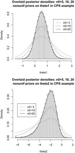MCMC sequences are easily computed in this case starting from the uniform prior, and it is easy to check that the distributions of the resulting sequence of simulated pairs $({\theta }_{1,k},{\theta }_{2,k})$ follow the analytical form (8(8) $\begin{array}{r}\{\exp (0.6{\theta }_1+0.05{\theta }_2)/(1+\exp ({\theta }_1)+\exp ({\theta }_2\left)\right){\}}^{n_0}\end{array}$(8) ) normalised by a numerically integrated constant of integration. The marginal histograms for ${\theta }_{1,k},{\theta }_{2,k}$ for $k=\mathrm{10,000}$ to $\mathrm{100,000}$ are shown in Figure 2 along with theoretical densities from (8(8) $\begin{array}{r}\{\exp (0.6{\theta }_1+0.05{\theta }_2)/(1+\exp ({\theta }_1)+\exp ({\theta }_2\left)\right){\}}^{n_0}\end{array}$(8) ) overlaid with the corresponding kernel density estimates for $n_0=5,10$.

Figure 2. Theoretical and (for $n_0=20$, MCMC-empirical) form of the nonuniform marginal prior densities induced by (8(8) $\begin{array}{r}\{\exp (0.6{\theta }_1+0.05{\theta }_2)/(1+\exp ({\theta }_1)+\exp ({\theta }_2\left)\right){\}}^{n_0}\end{array}$(8) ) for intercept parameters ${\theta }_1,{\theta }_2$ for $n_0=5,10,20$.

${\mathbf{2}}^{\mathbf{o}}$ Next we implemented the Metropolis-Hastings (M-H) algorithm in Steps 1–2 with the full 56-dimensional fixed-effect generalised logistic model, for the posterior $\pi \left(t|\mathcal{D}\right)$ under (1(1) $\begin{array}{r}P(Y_i=y|{\mathbf{X}}_i=\mathbf{x})=\exp \left({\mathbf{x}}^{\prime }{\text{β}}^{\left(y\right)}\right)/\left(1+\sum _{z=1}^{H-1}\exp \left({\mathbf{x}}^{\prime }{\text{β}}^{\left(z\right)}\right)\right)\end{array}$(1) )–(2(2) $\begin{array}{rl}P(Y_i& =H|{\mathbf{X}}_i=\mathbf{x})=1/\left(1+\sum _{z=1}^{H-1}\exp \left({\mathbf{x}}^{\prime }{\text{β}}^{\left(z\right)}\right)\right)\end{array}$(2) ) with $\mathit{\theta }=({\text{β}}^{\left(z\right)},z=1,2)$, using $\mathcal{N}(\hat{\mathit{\theta }},(\mathcal{I}\left(\hat{\mathit{\theta }}\right){)}^{-1})$ proposal density $q(\cdot )$. The algorithm with uniform improper prior on $\mathit{\theta }$ is implemented in this way on the original CPS dataset, but a completely analogous MCMC implementation using one of the priors ${\pi }_{n_0}$ requires only the single change that the dataset is augmented to have one more row corresponding to $n_0$ observations with covariate vector $\mathbf{X}={\mathbf{X}}_{\mathrm{a}\mathrm{v}\mathrm{g}}$ and outcome counts $(0.6n_0,0.05n_0,0.35n_0)$.

${\mathbf{3}}^{\mathbf{o}}$ Finally, we implemented the M-H algorithm with a 32-dimensional unknown parameter $\mathit{\alpha }$ where the 24 parameters $\mathit{\gamma }$ (those for terms other than the state intercepts) are fixed (at their MLEs). The equilibrium density for the MCMC sequence is now the posterior density of the conditional model (B) above, and the corresponding proposal density $q(\cdot )$ is $\mathcal{N}(\hat{\mathit{\alpha }},({\mathcal{I}}_{\mathit{\alpha }\mathit{\alpha }}\left(\hat{\mathit{\theta }}\right){)}^{-1})$ on ${\mathbb{R}}^{32}$.

Before reporting on data-analytic results, we collect several remarks related to acceptance rates and convergence in the MCMC implementations. Recall that the acceptance rate is the relative frequency with which successive ${\mathit{\theta }}_k,{\mathit{\theta }}_{k+1}$ variates differ in Step 2 of the M-H algorithm given above. This rate will be close to 1 when the proposal density is an excellent approximation of the desired posterior density. In calculations ${\mathbf{1}}^{\mathbf{o}}$ checking the theoretical priors (8(8) $\begin{array}{r}\{\exp (0.6{\theta }_1+0.05{\theta }_2)/(1+\exp ({\theta }_1)+\exp ({\theta }_2\left)\right){\}}^{n_0}\end{array}$(8) ) against posteriors calculated after $n_0=5,10$, or 20, we found acceptance respective rates $54.0\mathrm{\%},59.2\mathrm{\%},62.0\mathrm{\%}$, which are not bad considering that the asymptotic Laplace-method or Bernstein-von Mises approximation of posterior density is not close to the true posterior density when $n_0$ is small or moderate. In addition, as shown in Figure 2 for n = 20 (but not for $n_0=5,10$), there was good computational agreement between MCMC histograms and the theoretical marginal densities for ${\theta }_1,{\theta }_2$ after $T={10}^4$ burn-in iterations.

In the MCMC simulation ${\mathbf{2}}^{\mathbf{o}}$ of the 56-dimensional fixed-effect generalised logistic model, the acceptance rate in formula (7(7) ${\mathit{\theta }}_{k+1}={\mathit{\theta }}_k+(\tau -{\mathit{\theta }}_k)\cdot I\left[U\le \frac{\pi \left(\tau |\mathcal{D}\right)q\left({\mathit{\theta }}_k\right)}{\pi \left({\mathit{\theta }}_k|\mathcal{D}\right)q\left(\tau \right)}\right]$(7) ) was $51.7\mathrm{\%}$ and $51.2\mathrm{\%}$ in two runs of ${10}^5$ iterations on the CPS data. The rates were essentially the same ($52.7\mathrm{\%},52.4\mathrm{\%}$) when the simulation was re-run in the modified form with the prior ${\pi }_{20}$ in (8(8) $\begin{array}{r}\{\exp (0.6{\theta }_1+0.05{\theta }_2)/(1+\exp ({\theta }_1)+\exp ({\theta }_2\left)\right){\}}^{n_0}\end{array}$(8) ). The larger the parameter dimension, the harder it is to attain a high acceptance rate. A strategy of breaking the M-H step Gibbs-Sampler steps in the 56-dimensional variate generation into about 6 blocks improved the acceptance rate somewhat, of the order of $20\mathrm{\%}$, at the cost of much more computation. The single-step strategy in M-H Step 2 applied to the smaller parameter dimension of 44 of the fixed-effect model F1 resulted in acceptance rate of about $63\mathrm{\%}$. However, when the M-H simulation was run twice in the form ${\mathbf{3}}^{\mathbf{o}}$ with lower dimension 32, the acceptance rate was $42.6\mathrm{\%},42.8\mathrm{\%}$ in two runs with uniform prior and $42.7\mathrm{\%},42.3\mathrm{\%}$ in two runs with ${\pi }_{20}$ prior. Thus, the lower dimension in this case seems to have been offset by the slightly worse Bernstein-von Mises or Laplace approximation to the posterior density when the non-state-intercept parameters $\mathit{\gamma }$ were frozen at their MLEs.

Next we describe several indications of MCMC convergence, i.e., of the empirical distributions of $\{{\mathit{\theta }}_k{\}}_{k={10}^4}^{{10}^5}$ being very close to their stationary distributions which are the desired posterior and conditional posterior densities. The primary way of checking this convergence is to check that selected marginal empirical distributions are nearly the same for simulations with different starting points. We overplotted scaled relative frequency histograms of the sequence $\{{\mathit{\theta }}_{k,j}{\}}_{{10}^4}^{{10}^5}$ for each state effect coefficient j from one MCMC run with kernel-density estimates of the same state effect coefficient from another run (with band-widths determined from ${10}^4$ points, not ${10}^5$). We did this across pairs of runs, of type ${\mathbf{2}}^{\mathbf{o}}$ with flat priors and ${\pi }_{20}$ priors, and of type ${\mathbf{3}}^{\mathbf{o}}$ with flat priors and ${\pi }_{20}$ priors. In all of these pairwise comparisons, there is no visible difference between histograms versus densities from alternate runs of the same type. We also confirmed that the various averages and correlations described below were essentially the same for each of the pairs of runs of the same type.

The same histogram and kernel-density comparisons can also answer the question of whether the marginal posterior densities of the state intercepts show any differences for the MCMC runs of four different types, ${\mathbf{2}}^{\mathbf{o}}$ and ${\mathbf{3}}^{\mathbf{o}}$ each with either flat (uniform) prior or ${\pi }_{20}$ prior. On the CPS data, we saw no differences between the MCMC marginal posteriors of each of the two types ${\mathbf{2}}^{\mathbf{o}}$ and ${\mathbf{3}}^{\mathbf{o}}$ across different uniform or ${\pi }_{20}$ priors.

However, as in the discussion following (A)–(B) on page 20(6) $\begin{array}{rl}P(Y_i& =\mathrm{E}\mathrm{m}\mathrm{p}07|{\mathbf{X}}_{\mathrm{i}})=\mathrm{p}\mathrm{l}\mathrm{o}\mathrm{g}\mathrm{i}\mathrm{s}({\mathbf{X}}_{\mathrm{i}}^{\prime }{\text{β}}^{\left(1\right)})\\ & =\frac{\exp \left({\mathbf{X}}_i^{\prime }{\text{β}}^{\left(1\right)}\right)}{1+\exp \left({\mathbf{X}}_i^{\prime }{\text{β}}^{\left(1\right)}\right)}\end{array}$(6) , the posterior variances of state intercept coefficients ${\alpha }_j$ are smaller if the other (non-state-intercept) parameters $\mathit{\gamma }$ are regarded as fixed, by a factor $1/{\rho }_j^2$ one readily calculates as the ratio of state-intercept diagonal elements of the inverse observed information matrix $\mathcal{I}\left(\mathit{\theta }\right)$ when all parameters $\mathit{\alpha },\mathit{\gamma }$ are regarded as unknown divided by the corresponding state-intercept diagonal elements of the inverse $\left({\mathcal{I}}_{\mathit{\alpha }\mathit{\alpha }}\right(\mathit{\theta }){)}^{-1}$ of the information sub-matrix relating only to the state-intercept $\mathit{\alpha }$ parameters. These ratios are displayed in Table 3 for the 16 state intercepts $({\alpha }_1,\dots ,{\alpha }_{16})$ corresponding to the Emp outcome in the F2 model (1(1) $\begin{array}{r}P(Y_i=y|{\mathbf{X}}_i=\mathbf{x})=\exp \left({\mathbf{x}}^{\prime }{\text{β}}^{\left(y\right)}\right)/\left(1+\sum _{z=1}^{H-1}\exp \left({\mathbf{x}}^{\prime }{\text{β}}^{\left(z\right)}\right)\right)\end{array}$(1) )-(2(2) $\begin{array}{rl}P(Y_i& =H|{\mathbf{X}}_i=\mathbf{x})=1/\left(1+\sum _{z=1}^{H-1}\exp \left({\mathbf{x}}^{\prime }{\text{β}}^{\left(z\right)}\right)\right)\end{array}$(2) ). In that same Table, we display also the various empirical posterior means of ${\alpha }_j$ based on MCMC simulation of type ${\mathbf{2}}^{\mathbf{o}}$ with flat prior and with ${\pi }_{20}$ prior (respectively denoted Unif .${\mathbf{2}}^{\mathbf{o}}$ and ${\pi }_{20}$.${\mathbf{2}}^{\mathbf{o}}$ in column-headers) and of type ${\mathbf{3}}^{\mathbf{o}}$ with flat prior (denoted Unif .${\mathbf{3}}^{\mathbf{o}}$), where theory says that all of these means should be approximately the same as the corresponding MLEs ${\hat{\alpha }}_j$ in large-sample data. (Note also that the MLEs are the ${\alpha }_j$ values for the true mode of the posterior joint density, while the Unif .${\mathbf{2}}^{\mathbf{o}}$ and Unif .${\mathbf{3}}^{\mathbf{o}}$ columns show corresponding Monte Carlo estimates of the ${\alpha }_j$ posterior means.) To correct for predicted differences in standard deviations, we overplot in Figure 3 against the marginal empirical histograms (for all indices k) of the state intercept coefficients a density estimate for the rescaled elements (9) ${\hat{\mathit{\theta }}}_j+{\hat{\rho }}_j({\theta }_{k,j}-{\hat{\mathit{\theta }}}_j)$(9) Here ${\hat{\mathit{\theta }}}_j$ is the MLE for a state intercept, and $\{{\theta }_{k,j}{\}}_{k={10}^4}^{{10}^5}$ denotes the corresponding simulated sequence of type ${\mathbf{3}}^{\mathbf{o}}$ with non-state-intercept parameters $\mathit{\gamma }$ fixed at their MLEs $\hat{\mathit{\gamma }}$, and ${\hat{\rho }}_j$ is the ratio of the estimated standard error of ${\hat{\mathit{\theta }}}_j$ when $\mathit{\gamma }$ is not fixed over that when $\mathit{\gamma }$ is fixed.

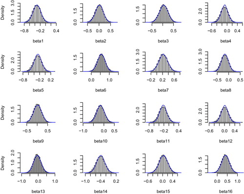
Figure 3. Plots for 16 state intercept coefficients for outcome Emp in F2 model (1(1) $\begin{array}{r}P(Y_i=y|{\mathbf{X}}_i=\mathbf{x})=\exp \left({\mathbf{x}}^{\prime }{\text{β}}^{\left(y\right)}\right)/\left(1+\sum _{z=1}^{H-1}\exp \left({\mathbf{x}}^{\prime }{\text{β}}^{\left(z\right)}\right)\right)\end{array}$(1) )–(2(2) $\begin{array}{rl}P(Y_i& =H|{\mathbf{X}}_i=\mathbf{x})=1/\left(1+\sum _{z=1}^{H-1}\exp \left({\mathbf{x}}^{\prime }{\text{β}}^{\left(z\right)}\right)\right)\end{array}$(2) ), with (bounded-range) Uniform prior, of marginal posterior histogram of simulated type ${\mathbf{2}}^{\mathbf{o}}$ parameter versus kernel density estimator of type ${\mathbf{3}}^{\mathbf{o}}$ simulated parameters rescaled as in (9(9) ${\hat{\mathit{\theta }}}_j+{\hat{\rho }}_j({\theta }_{k,j}-{\hat{\mathit{\theta }}}_j)$(9) ).

Table 3. MLEs and MCMC posterior means (of 3 types) for state intercepts in outcome Emp in F2 model (1(1) $\begin{array}{r}P(Y_i=y|{\mathbf{X}}_i=\mathbf{x})=\exp \left({\mathbf{x}}^{\prime }{\text{β}}^{\left(y\right)}\right)/\left(1+\sum _{z=1}^{H-1}\exp \left({\mathbf{x}}^{\prime }{\text{β}}^{\left(z\right)}\right)\right)\end{array}$(1) )–(2(2) $\begin{array}{rl}P(Y_i& =H|{\mathbf{X}}_i=\mathbf{x})=1/\left(1+\sum _{z=1}^{H-1}\exp \left({\mathbf{x}}^{\prime }{\text{β}}^{\left(z\right)}\right)\right)\end{array}$(2) ).

			Posterior means			SDratio
FIPS	State	MLE	Unif .${\mathbf{2}}^{\mathbf{o}}$	${\pi }_{20}$.${\mathbf{2}}^{\mathbf{o}}$	Unif .${\mathbf{3}}^{\mathbf{o}}$	${\hat{\rho }}_j$
01	AL	−0.323	−0.335	−0.336	−0.321	1.15
04	AZ	0.016	0.006	0.005	0.016	1.09
09	CT	0.049	0.040	0.038	0.051	1.05
13	GA	−0.095	−0.106	−0.107	−0.095	1.14
22	LA	−0.263	−0.275	−0.277	−0.262	1.15
23	ME	0.559	0.553	0.549	0.557	1.05
25	MA	0.227	0.217	0.216	0.228	1.11
28	MS	−0.163	−0.175	−0.174	−0.161	1.14
32	NV	0.022	0.011	0.013	0.021	1.08
33	NH	−0.163	−0.175	−0.173	−0.155	1.08
35	NM	−0.225	−0.238	−0.236	−0.224	1.13
37	NC	0.010	0.000	−0.001	0.011	1.13
44	RI	−0.057	−0.063	−0.067	−0.052	1.05
45	SC	−0.402	−0.413	−0.414	−0.399	1.11
49	UT	0.034	0.024	0.023	0.036	1.09
50	VT	0.414	0.404	0.402	0.413	1.07

Notes: Final column is ratio of estimated standard errors of MLEs when parameters $\mathit{\gamma }$ are not or are fixed.

2.5.2. Results of Bayesian data analysis

The pairs of marginal empirical histograms and density estimates referenced above for state intercept parameters for the most part look very close to normally distributed, for all states and for those parameters both in the Emp (i.e., z = 1) and the Unemp (z = 2) terms in model (1(1) $\begin{array}{r}P(Y_i=y|{\mathbf{X}}_i=\mathbf{x})=\exp \left({\mathbf{x}}^{\prime }{\text{β}}^{\left(y\right)}\right)/\left(1+\sum _{z=1}^{H-1}\exp \left({\mathbf{x}}^{\prime }{\text{β}}^{\left(z\right)}\right)\right)\end{array}$(1) ). We do not show these sets of histogram and density-estimate pairs because they are visually indistinguishable across priors and multiple runs of the M-H simulations. However, for the Unif .${\mathbf{2}}^{\mathbf{o}}$ and rescaled Unif .${\mathbf{3}}^{\mathbf{o}}$ simulated M-H sequences described above as in (9(9) ${\hat{\mathit{\theta }}}_j+{\hat{\rho }}_j({\theta }_{k,j}-{\hat{\mathit{\theta }}}_j)$(9) ), there are some slight differences. Inspection of Figure 3 shows that for states 4, 5, 11 and to a lesser extent also 8, the blue rescaled-variate density estimates are more peaked in the middle than the corresponding histograms, while the histograms appear slightly more peaked in the plots for states 9 and 13. However, all of the differences are small and seem likely due to sampling variability of the estimated standard-deviation ratios ${\hat{\rho }}_j$.

It remains to present results concerning posterior dependence between parameters, and their relevance for the choice of random-effect distributions in the frequentist analyses of Section 2.4. We briefly describe correlational results, which for the most part confirm theoretical large-sample predictions using the asymptotic normal MLE distribution; then draw what information we can from the empirical mixture distribution of state intercepts within each of the z = 1 and z = 2 terms of model (1(1) $\begin{array}{r}P(Y_i=y|{\mathbf{X}}_i=\mathbf{x})=\exp \left({\mathbf{x}}^{\prime }{\text{β}}^{\left(y\right)}\right)/\left(1+\sum _{z=1}^{H-1}\exp \left({\mathbf{x}}^{\prime }{\text{β}}^{\left(z\right)}\right)\right)\end{array}$(1) ) along with its implications for frequentist random-effects modelling; and finally, we close with a few results concerning Bayesian predictions for small gross-flow cell counts.

First, the priors ${\pi }_{n_0}$ for $n_0>0$ already induce dependence between the two overall intercept parameters ${\theta }_z={\mathbf{X}}_{\mathrm{a}\mathrm{v}\mathrm{g}}^{\prime }{\text{β}}^{\left(z\right)},z=1,2$. Using the M-H simulations of type ${\mathbf{1}}^{\mathbf{o}}$, checked by direct numerical integration of the expression (2), we find correlation between ${\theta }_1,{\theta }_2$ of respectively 0.17, 0.20, 0.23 for $n_0=5,10,20$.

Next, we consider the dependence among state-intercept parameters in the fixed-effect ML and the Bayes-posterior frameworks. A first observation is that for all j the correlations between state-intercept parameter ML estimates ${\widehat{\text{β}}}_j^{\left(1\right)},{\widehat{\text{β}}}_j^{\left(2\right)}$ for the Emp07 and Unemp07 outcomes (from the asymptotic variance matrix $\left(\hat{\mathcal{I}}\right(\hat{\mathit{\theta }}){)}^{-1}$) are about 1/3, and the same is true for the analogous correlations according to the Bayes posteriors for both the full-Bayes (56-dimensional) and conditional Bayes (fixing the $\mathit{\gamma }$ parameters), with all choices of priors we tried. Among the distinct state intercepts within the Emp07 outcome, the ML state-intercept correlations are fairly small (no more than 0.10 in magnitude) and consistently negative. Under the full-Bayes posterior, with either the Uniform or ${\pi }_{20}$ prior, the corresponding correlations are all positive from 0.09 to 0.27, with their mean and median between 0.17 and 0.18. On the other hand, under the Bayes posteriors constructed with non-state-intercept parameters $\mathit{\gamma }$ fixed, the correlations are all uniformly small, between $-0.02$ and 0.02. This seems to say that the sizeable correlations among distinct state-intercepts for the full F2 model are largely induced through the variability of the non-fixed $\mathit{\gamma }$ parameters. The posterior near-independence of state-intercepts for different states under fixed $\mathit{\gamma }$ accords well with the model assumption made in random-effects extensions of the F2 model, with the proviso that the random effects for the state-intercept of each state across the two outcomes Emp07, Unemp07 need to be assumed dependent.

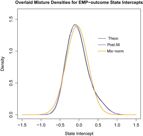
Further guidance can be found in the Bayesian posterior analysis concerning the distributional shape of random state-intercept effects in the CPS data. A natural, but we believe novel, approach is to approximate a common random-effect distribution by the mixture of normal distributions centred at the ML-fitted state intercepts with standard deviations equal to those taken from the inverse information matrix as given by asymptotic MLE and Bernstein-von Mises theory. Restricting attention to the 16 state intercepts within the Emp07 terms (z = 1) in model (1(1) $\begin{array}{r}P(Y_i=y|{\mathbf{X}}_i=\mathbf{x})=\exp \left({\mathbf{x}}^{\prime }{\text{β}}^{\left(y\right)}\right)/\left(1+\sum _{z=1}^{H-1}\exp \left({\mathbf{x}}^{\prime }{\text{β}}^{\left(z\right)}\right)\right)\end{array}$(1) ), this mixed density with weights proportional to state sample size is plotted as the black line labelled ‘Theor’ in Figure 4. We compare with that the mixture across states (again with sample-size weights) of the posterior density estimates from the Bayesian MCMC simulation of type ${\mathbf{2}}^{\mathbf{o}}$, which is plotted in blue in Figure 4. Finally, we compare both of these with the orange normal density line sharing mean $-0.054$ and standard deviation 0.285 of the black mixed-normal density. Figure 4 indicates clearly that the overall posterior mixed distribution of state-intercepts is approximately normal, supporting the idea of a mixed-effects frequentist model.

Figure 4. Figure showing near normality of mixed state-effect density across different states.

2.5.3. Predictions

Now consider the way in which the fitted fixed-effects F2 model leads by frequentist or Bayesian analysis to predictions of gross-flow cell counts in the CPS data. All of the predictions we discuss in this Section, like all of the methods considered in this paper, are conditional given $\{{\mathbf{X}}_i,Y_{i+}{\}}_i$, while in survey applications, the variability of survey-weighted totals related to ${\mathbf{X}}_i$ would generally be estimated by design based methods such as Balanced Repeated Replication (BRR), as in Thibaudeau et al. (2017, 2019). Another important point is that in survey applications, design-based survey weighting and not models would generally be used for prediction in the largest cells, such as the age and education groups that were employed in both months of the June–July 2017 CPS data. For this reason, the survey origin of the data leads to unusual metrics, focussed on small gross-flow cells, for comparative predictive success of models.

As an illustration of the small-cell predictions, consider three gross-flow cells corresponding to those in EMP status in July 2017 respectively for the No-college 35-54 age-group in NILF labour-status in June 2017 in the two states of Louisiana (LA) and New Mexico (NM), and in the combination across all 16 states (denoted ALL in Figure 5 below) of the No-college 55-64 age-group in UNEMP labour-status in June 2017. The total counts across all July labour-categories in these STAT06 x AGE06 x EDUC06 groups are respectively 100 for LA, 70 for NM, and 40 for ALL, after rounding to the nearest 10. The numbers in Emp07 status in July are $<15$ for all three LA, NM and ALL gross-flow cells. The predicted cell counts for the three gross-flow cells, based on treating the STAT06 x AGE06 x EDUC06 group counts as known and substituting the MLEs $\hat{\mathit{\theta }}$ for the F2 model (1(1) $\begin{array}{r}P(Y_i=y|{\mathbf{X}}_i=\mathbf{x})=\exp \left({\mathbf{x}}^{\prime }{\text{β}}^{\left(y\right)}\right)/\left(1+\sum _{z=1}^{H-1}\exp \left({\mathbf{x}}^{\prime }{\text{β}}^{\left(z\right)}\right)\right)\end{array}$(1) )–(2(2) $\begin{array}{rl}P(Y_i& =H|{\mathbf{X}}_i=\mathbf{x})=1/\left(1+\sum _{z=1}^{H-1}\exp \left({\mathbf{x}}^{\prime }{\text{β}}^{\left(z\right)}\right)\right)\end{array}$(2) ), are respectively 4.70 for LA, 3.48 for NM, and 3.83 for ALL.

Figure 5. Three histograms showing Bayes predictions of small gross-flow cells.

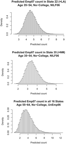
While standard errors for these predicted counts could be developed using the delta-method in terms of the asymptotic variance of $\hat{\mathit{\theta }}$, we use instead the posterior distributions of the predictors in Figure 5. The histograms shown there are based on posterior MCMC simulations of length ${10}^5$ (after burn-in of ${10}^5$) of type ${\mathbf{2}}^{\mathbf{o}}$ with Uniform prior and summarise the distributions of the three small-cell predictions. The three respective posterior mean and standard-deviation pairs are $(4.68,0.76),(3.46,0.60)$, and $(3.81,1.39)$. Note that the three posterior densities shown for the predictors are clearly non-normal.

3. Discussion

This paper has contrasted fixed- and mixed-effect (generalised) logistic conditional probability models on a two-period three-outcome longitudinal CPS survey dataset covering 16 states, using likelihood-based and predictive metrics, both frequentist and Bayesian. The findings from fixed-effect analyses with state effects, from corresponding models with state random effects, and fom Bayes analysis of posteriors for the fixed state-effects with other model coefficients fixed, all confirm each other and support a model with normal random state effects, independent across states. The analyses reinforce one another, suggesting that in these data, there is only one important (fixed-effect, pairwise) interaction – between labour status STAT06 in the earlier time-period and age-group dummy indicators AGE06 – and fairly weak but non-negligible (and statistically significant) area (State) effects. The dataset is large enough that a fixed-effects model incorporating areas could be used, but a simple random-intercept model (with independent intercepts for the two separate Emp07 and Unemp07 outcomes contrasted with NILF07) is just as good for predictive purposes, as is confirmed by the Bayesian analysis. As often happens with (nearly) statistically adequate models on large datasets with only slight BIC differences, the predictions from the simplest models are almost indistinguishable from those of the more richly parameterised models, including the random-effect models.

One reason to prefer the fixed-effect conditional models studied in this paper is that they lend themselves to simple linearised variances for predicted cell totals as in Thibaudeau et al. (2017), while the corresponding variances for predictions under mixed-effect models are more problematic due to the survey weighting, a topic that has already been explored and highlighted in previous research (Slud & Ashmead, 2017; Slud, Ashmead, Joyce, & Wright, 2018). For the fixed-effect models, both the predictions and their standard errors are also handily derived using a Bayesian MCMC approach, as has been demonstrated for a few small cells in the CPS data.

Disclosure statement

No potential conflict of interest was reported by the authors.

Additional information

Notes on contributors

Eric Slud

Eric Slud is Area Chief for Mathematical Statistics in the Center for Statistical Research and Methodology of the US Census Bureau, and is Professor in the Statistics Program within the Mathematics Department of the University of Maryland, College Park.

Yves Thibaudeau

Yves Thibaudeau is a Mathematical Statistician and Principal Researcher in the Center for Statistical Research and Methodology at the US Census Bureau.

References

- Agresti, A. (2013). Categorical data analysis. Hoboken, NJ: Wiley.
- Bickel, P., & Doksum, K. (2015). Mathematical statistics: Basic ideas and slected topics (2nd ed. Vol. I). Boca Raton, FL: Chapman & Hall/CRC.
- Casella, G., & Robert, C. (2005). Monte Carlo statistical methods (2nd Ed.). New York: Springer.
- Fienberg, S. (1980). The measurement of crime victimization: Prospects for a panel analysis of a panel survey. Journal of the Royal Statistical Society Series D, 29, 313–350.
- Gelman, A., & Hill, J. (2007). Data analysis using regression and multilevel/hierarchical models. New York: Cambridge Univ. Press.
- Hand, D., & Till, R. (2001). A simple generalization of the area under the ROC curve for multiple class classification problems. Machine Learning, 45(2), 171–186. doi: 10.1023/A:1010920819831
- Li, J., & Fine, J. (2008). ROC analysis with multiple classes and multiple tests: Methodology and its application in microarray studies. Biostatistics, 9, 566–576. Retrieved from https://doi.org/10.1093/biostatistics/kxm050
- Pfeffermann, D., Skinner, C., & Humphreys, K. (1998). The estimation of gross flows in the presence of measurement error using auxiliary variables. Journal of the Royal Statistical Society Series A, 161, 13–32. doi: 10.1111/1467-985X.00088
- Pinheiro, J., & Bates, D. (1995). Approximations of the loglikelihood function in the nonlinear mixed effects model. Journal of Computational and Graphical Statistics, 4, 12–35.
- Rao, J. N. K, & Molina, I. (2015). Small area estimation (2nd ed.). Hoboken, NJ: John Wiley.
- R Core Team (2017). R: A language and environment for statistical computing. R Foundation for Statistical Computing, Vienna, Austria. Retrieved from https://www.R-project.org/
- Särndal, C.-E., Swensson, J., & Wretman, J. (1992). Model assisted survey estimation. New York: Springer.
- Self, S., & Liang, K.-Y. (1987). Asymptotic properties of maximum likelihood estimators and likelihood ratio tests under nonstandard conditions. Journal of the American Statistical Association, 82, 605–610. doi: 10.1080/01621459.1987.10478472
- Slud, E., & Ashmead, R. (2017). Hybrid BRR and parametric-bootstrap variance estimates for small domains in large surveys. Proceedings of American Statistical Association, Survey Research Methods Section, Alexandria, VA, pp. 1716–1730.
- Slud, E., Ashmead, R., Joyce, P., & Wright, T. (2018). Statistical methodology (2016) for Voting Rights Act Section 203 determinations (Research Report Series RRS2018/12). Center for Statistical Research and Methodology, US Census Bureau.
- Stroup, W. (2013). Generalized linear mixed models. Boca Raton, FL: Chapman & Hall/CRC.
- Thibaudeau, Y., Slud, E., & Cheng, Y. (2019). Small-area estimation of cross-classified gross flows using longitudinal survey data. In P. Lynn (Ed.), Methodology of longitudinal surveys II. New York: Wiley.
- Thibaudeau, Y., Slud, E., & Gottschalck, A. (2017). Modeling log-linear conditional probabilities for estimation in surveys. The Annals of Applied Statistics, 11, 680–697. doi: 10.1214/16-AOAS1012